Changes in Physical Parameters of CO₂ Containing Impurities in the Exhaust Gas of the Purification Plant and Selection of Equations of State

Abstract

CO₂ transport is a crucial part of CCUS. Nonetheless, due to the physical property differences between CO₂ and natural gas and oil, CO₂ pipeline transport is distinct from natural gas and oil transport. Gaseous CO₂ transportation has become the preferred scheme for transporting impurity-containing CO₂ tail gas in purification plants due to its advantages of simple technology, low cost, and high safety, which are well suited to the scenarios of low transportation volume and short distance in purification plants. The research on its physical property and state parameters is precisely aimed at optimizing the process design of gaseous transportation so as to further improve transportation efficiency and safety. Therefore, it has important engineering practical significance. Firstly, this paper collected and analyzed the research cases of CO₂ transport both domestically and internationally, revealing that phase state and physical property testing of CO₂ gas containing impurities is the basic condition for studying CO₂ transport. Subsequently, the exhaust gas captured by the purification plant was captured after hydrodesulfurization treatment, and the characteristics of the exhaust gas components were obtained by comparing before and after treatment. By preparing fluid samples with varied CO₂ content and conducting the flash evaporation test and PV relationship test, the compression factor and density of natural gas under different temperatures and pressures were obtained. It is concluded that under the same pressure in general, the higher the CO₂ content, the smaller the compression factor. Except for pure CO_2, the higher the CO₂ content, the higher the density under constant pressure, which is related to the content of C₂ and heavier hydrocarbon components. At the same temperature, the higher the CO₂ content, the higher the viscosity under the same pressure; the lower the pressure, the slower the viscosity growth slows down. The higher the CO₂ content at the same temperature, the higher the specific heat at constant pressure. With the decrease in temperature, the CO₂ content reaching the highest specific heat at the identical pressure gradually decreases. Finally, BWRS, PR, and SRK equations of state were utilized to calculate the compression factor and density of the gas mixture with a molar composition of 50% CO₂ and the gas mixture with a molar composition of 100% CO₂. Compared with the experimental results, the most suitable equation of state is selected as the PR equation, which refers to the parameter setting of critical nodes of CO₂ gas transport.

1. Introduction

Recently, China’s energy policies have undergone restructuring. In this context, there will be substantial growth in natural gas consumption. Simultaneously, more carbon dioxide emissions will arise in sectors such as coal-to-chemicals and power generation. Carbon capture and storage (hereinafter referred to as CCS) technology is acknowledged as the most viable solution to implement CO₂ emission reduction globally [1,2,3,4]. Pipeline transport of CO₂ is extremely crucial to the CCS technology chain [5,6,7]. In 1984, Texaco, an American company, pioneered building the CO₂ gas transport pipeline worldwide, with the objective of testing CO₂-EOR at Paradis [8]. In 1986, the Bairoil Oilfield in Wyoming, USA, commenced injecting carbon dioxide. The criteria for CO₂ transport in this pipeline are as follows: CO₂ ≥ 98 mol%, N ≤ 0.5 mol%, and CH₄ = 1–1.5 mol% [9]. Beaver Creek [10] is one of the deepest CO₂ enhanced oil recovery (EOR) projects in the United States. In July 2008, the project commenced operations through gas flooding. The Quest project is the inaugural commercial-scale carbon capture and storage project in the heavy oil industry [11]. The United States has amassed over 30 years of experience in CO₂ pipeline transport. Canada, Norway, and other countries have also carried out relevant work. However, China is still in the initial stage. Most of the CO₂ pipelines that have been operated only support short-distance transport, and most of them are used for oilfield EOR. There are no long-distance CO₂ transport pipelines [11,12,13,14,15,16,17]. The overall costs would be substantially reduced if modifications were made to existing pipelines [18,19]. Concerning gas-phase pipeline transport, there are low specifications for pipeline materials, CO₂ impurities, and pressure ratings. Gas-phase pipeline is safe and suitable for short-distance and low-volume transport [20,21]. Hence, the CO₂ containing impurities in the exhaust gas of the purification plant can be transported via the gas-phase pipeline.

Natural gas and oil transport pipelines have functioned securely and efficiently for decades, demonstrating high-level security and reliability and thereby serving as a reference for CO₂ pipeline transport in some measure. However, CO₂ still shows specificity towards natural gas and oil owing to their distinct physical properties. There are, inevitably, other gas impurities (e.g., SOX, NOX, O₂, H₂S, N₂, etc.) present in CO₂ transport pipelines [22,23]. Unlike oil and gas transport pipelines, CO₂ fluid acts as the predominant phase in CO₂ transport pipelines. The interaction with other impurities in the pipeline and the changes in physicochemical properties with the environment markedly differ from those of oil and gas pipelines. Moreover, significant disparities exist in CO₂ pipeline transport with different phases [24] and impurity effects [25]. So far, several problems still exist in CO₂ pipeline transport [26,27]: there is notably insufficient research exploring the effects of the phase transition mechanism and thermodynamic properties of CO₂ containing impurities on fracture extension. Most of the research models ignore the effect of impurities.

The mechanism of impurity influence is investigated regarding the possible presence of gas impurities, such as H₂O, N₂, H₂, CO, COS, and H₂S, in the tail gas of the purification plant. The prediction error of Span and Wagner [28] for physical properties such as phase boundary, critical point, density, and heat capacity of pure CO₂ is less than 0.1%, which provides a reference system for the study of the influence of impurities. Fenghour et al. [29] collected and summarized the viscosity data containing impurity CO₂ and found that the ranking of the influence of impurities on viscosity was H₂O > H₂S > CH₄ > N₂. Kontogeorgis and Folas [30] found that polar impurities (such as H₂O, SO₂) need to introduce association terms or polarity correction. The binary interaction parameters of light gas impurities (N₂, CH₄) are strongly correlated with the differences in molecular size. Li and Jakobsen [31] found in their research that when H₂O > 500 ppm, the critical trajectory was significantly changed, increasing the critical pressure by 10–15%. H₂O enhances the viscosity of the mixture through a hydrogen bond network. Gernert and Span [32] developed a CO₂ mixture model containing H₂O, N₂, and O₂ (EOS-CG) and concluded that light gas impurities reduced the Joule–Thomson coefficient, which might affect the cooling rate of the pipeline. Ahmadi and Chapoy [33] concluded that H₂S causes the critical temperature of CO₂ to rise and the critical pressure to drop. The H₂S-CO₂ mixture is prone to forming eutropic points, which leads to difficulties in phase separation.

Therefore, studying the physical property and state parameters of impurity-containing CO₂ tail gas from purification plants is of crucial importance, as it directly determines the safety and efficiency of pipeline transportation. Impurities can significantly alter the phase behavior of CO₂ mixtures, helping to avoid the formation of liquid slugs or solid blockages in the pipeline during transportation. They also affect key transportation parameters, ensuring the accuracy of pressure drop calculations and the selection of power equipment. Moreover, they are related to the risk of material corrosion, guiding the setting of dehydration depth and anti-corrosion measures. Mastering these physical properties forms the basis for scientifically setting core parameters of the pipeline, such as pressure, temperature, and flow rate, thereby ensuring the safe and stable operation of the entire transportation system.

2. Characteristics of Components Before and After Carbon Capture in the Exhaust Gas of X Purification Plant

2.1. Components of Hydrodesulfurization Exhaust Gas

The exhaust gas captured by the X Purification Plant, after undergoing hydrodesulfurization, generally has a CO₂ content below 50% and contains a large number of impurities. The components of exhaust gas in the X Purification Plant are presented in

Table 1. Components of hydrodesulfurization exhaust gas.

Components	CO2	H2O	N2	H2	CO	COS	H2S	Total
Content mol%	42.2644	5.2810	49.3489	2.4568	0.1013	0.0032	0.0140	100

:

By analyzing the components of the exhaust gas of the company’s X Purification Plant, we discovered that the exhaust gas exhibits a moderate to low-level concentration of CO₂ and a substantial presence of N₂. Additionally, there may be impurities such as H₂O, H₂S, COS, CO, and H₂ in the exhaust gas, and H₂O accounts for a higher proportion. During transportation, CO₂ hydrates are highly prone to forming, rendering direct pipeline transport infeasible. Thus, it is vital to conduct carbon capture on the exhaust gas to eliminate impurities and acquire high-purity CO₂.

2.2. Components After Carbon Capture

Prior to transportation, the captured CO₂ shall undergo the purification and drying treatment process. In general, the CO₂ concentration can exceed 95% with minimal impurity content. The components of CO₂ after carbon capture are shown in

Table 2. Components of CO₂ after carbon capture in the company’s X Purification Plant.

Components	CO2	H2O	N2	H2	CO	COS	H2S	Total
Content mol%	99.9883	0.0017	0.0089	0.0006	0.0001	0.0001	0.0003	100

:

In the CO₂ mixture after carbon capture, the molar composition of CO₂ exceeds 98%, with the majority of impurities removed. There remain only trace amounts of gas impurities like N₂, H₂O, H₂S, COS, CO, H₂, and light hydrocarbons.

3. Phase State and Physical Property Test of CO₂ Gas Containing Impurities

3.1. Experimental Test Samples and Methods

3.1.1. Experimental Test Sample

The experimental gas was synthesized by a laboratory using captured CO₂ and natural gas purified by the X Purification Plant. Fluid samples with various CO₂ content were prepared using six gases, including 10% CO₂, 30% CO₂, 50% CO₂, 70% CO₂, 90% CO_2, and pure CO₂. Natural gas components with varying CO₂ content were measured through gas chromatography, as seen in

Table 3. Molar composition (%) of natural gas with different CO₂ content.

CO2 Content (%)	100	90	70	50	30	10
CO2	100	91.77	70.98	50.99	28.86	9.84
N2	-	0.58	1.14	0.83	1.24	2.05
C1	-	-	27.32	46.54	67.73	86.02
C2	-	7.60	0.46	1.16	1.59	1.67
C3	-	-	0.08	0.33	0.42	0.31
iC4	-	0.02	0.01	0.05	0.06	0.04
nC4	-	-	0.01	0.06	0.07	0.05
iC5	-	-	0.01	0.02	0.03	0.01
nC5	-	-	-	0.01	0.01	-
C6+	-	0.02	-	0.01	-	-

:

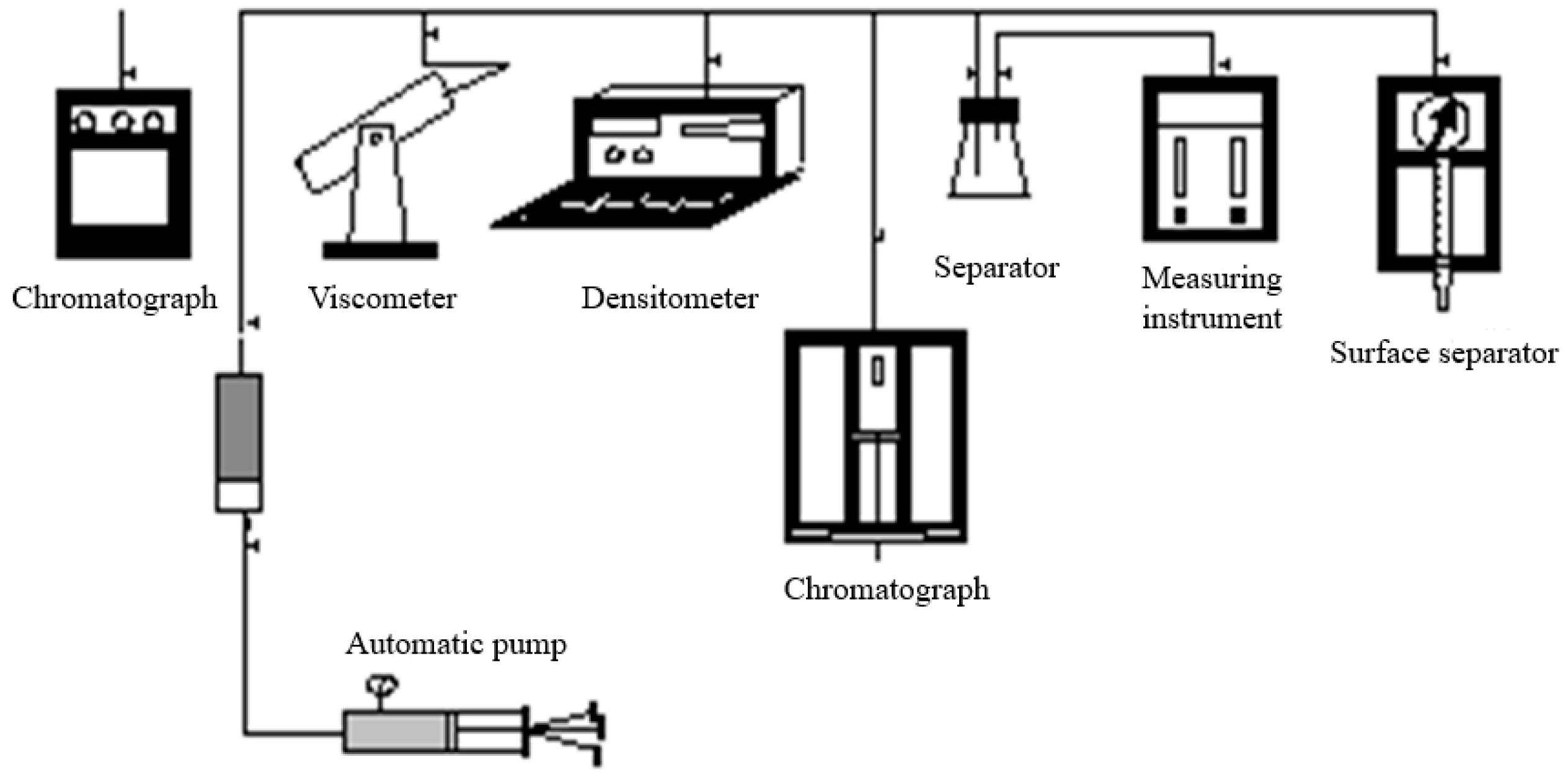
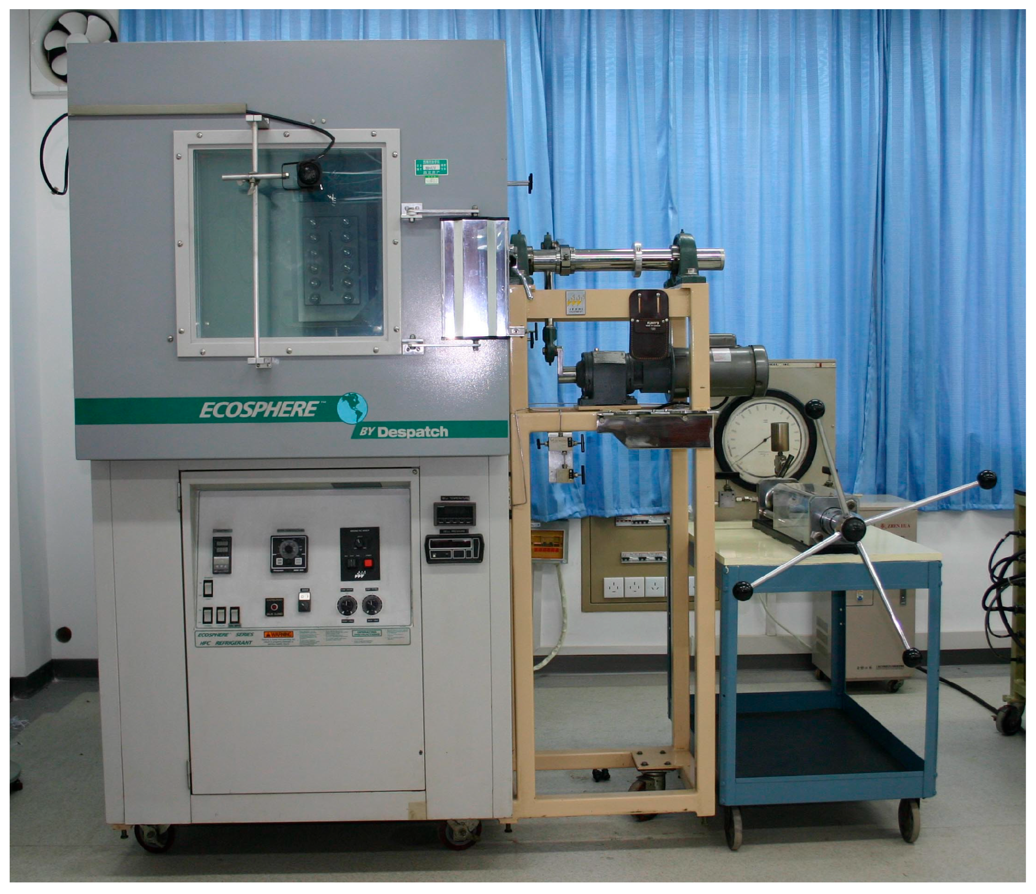
3.1.2. Experimental Setup and Testing Methods

Utilizing the flash evaporation test and PV relationship test, the physical property parameters, including viscosity, compression factor, and density of natural gas at various temperatures and pressures, can be obtained. The natural gas PVT experimental test was carried out in the JEFRI mercury-free high-temperature and high-pressure formation fluid analyzer with an observation window developed and produced by the DBR Company of Canada (Hamilton, ON, Canada). This process mainly consists of an injection pump system, a PVT cylinder, a flash separator, a density meter, a temperature control system, a gas chromatograph, an electronic balance, and a gas booster pump. The experimental setup and process are shown in Figure 1 and Figure 2.

The experimental tests were performed in accordance with China’s oil and gas industry standard ISO 20486:2017 [34]. In terms of error control, we reduce non-representative errors from the sampling source, strictly follow the experimental standards, and ensure that the experimental conditions, operators, and data processing logic are traceable.

3.2. Experimental Results and Physical Property Trends of Compression Factor

3.2.1. Experimental Results

For exhaust gas containing impurities with a temperature range of 0~60 °C, CO₂ content of 10~100%, and a pressure range of 1~33 MPa, the compression factor changes are illustrated in Figure 3:

3.2.2. Compression Factor Changes in CO₂ Containing Impurities

(1)

The compression factor diminishes with the rising pressure and subsequently increases after reaching the critical value.

(2)

The lower the temperature, the smaller the critical compression factor for a given CO₂ content, and the lower the critical pressure when the critical compression factor is reached.

(3)

At a constant temperature, the higher the CO₂ content, the smaller the compression factor when the critical pressure is reached. Typically, the higher the CO₂ content at the same pressure, the smaller the compression factor. Comparatively, the compression factor of pure CO₂ is higher than that of 90% CO₂ at 20 °C and 0 °C under the same pressure (provided that the pressure exceeds 15 MPa and 5 MPa, respectively) due to the fact that 90% CO₂ contains more C₂ and heavier components.

3.3. Experimental Results and Physical Property Trends of Density

3.3.1. Experimental Results

For exhaust gas containing impurities with a temperature range of 0~60 °C and a CO₂ content of 10~100%, the density changes at a pressure range of 1~33 MPa are depicted in Figure 4:

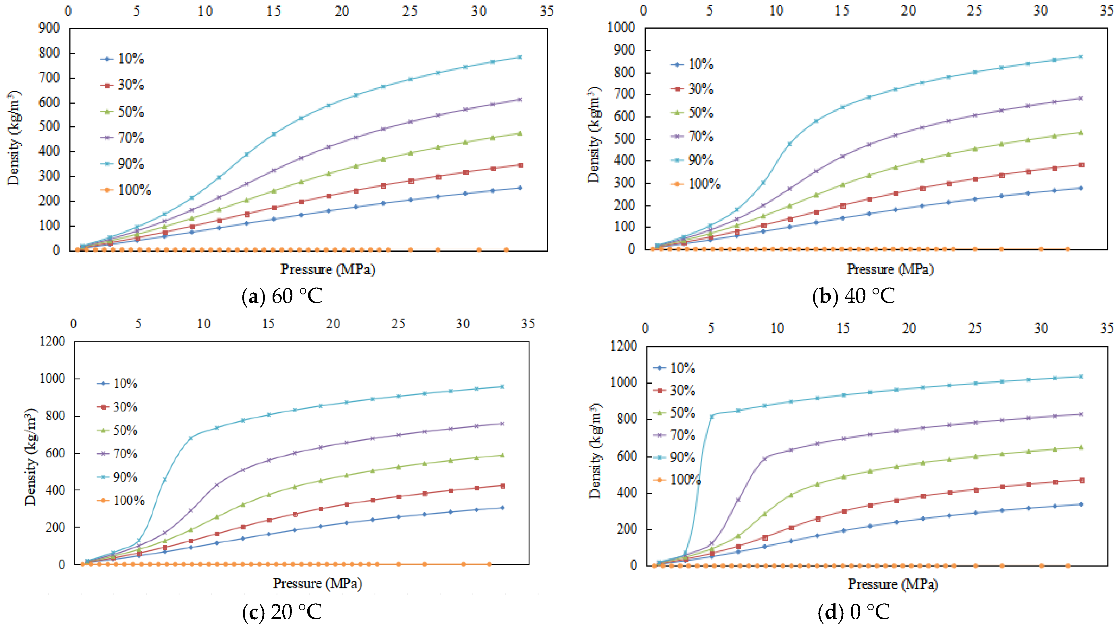
3.3.2. Density Changes of CO₂ Containing Impurities

(1)

As pressure escalates, density rises at a faster rate, followed by a gradual deceleration.

(2)

The density of a given CO₂ content is higher at lower temperatures.

(3)

At a constant temperature, for gas mixtures excluding pure CO₂, higher CO₂ content leads to a higher density under the same pressure. This phenomenon is linked to the presence of C₂ and heavier hydrocarbons in the exhaust gas from purification plants.

3.4. Experimental Results and Physical Property Trends in Viscosity

3.4.1. Experimental Results

For exhaust gas containing impurities with a temperature range of 0~60 °C, CO₂ content of 10~100%, and a pressure range of 1~33 MPa, the viscosity changes are illustrated in Figure 5:

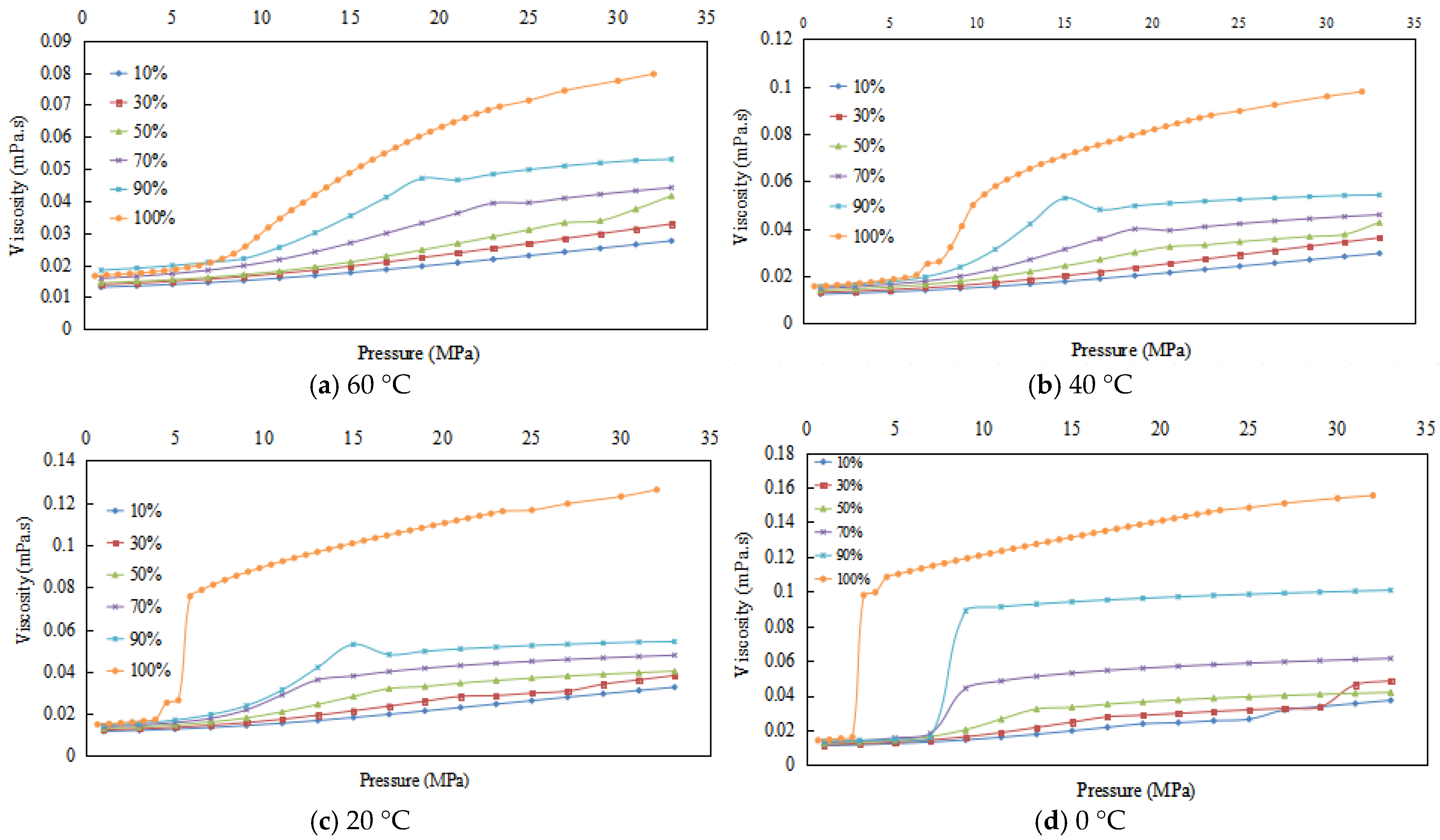
3.4.2. Viscosity Changes of CO₂ Containing Impurities

(1)

Viscosity increases with pressure, with the growth rate changing from slow to fast, then slowing again.

(2)

The lower the temperature, the higher the viscosity of the given CO₂ content under the same pressure, and the lower the pressure at which viscosity growth slows.

(3)

At the same temperature, the higher the CO₂ content, the higher the viscosity under the same pressure, and the lower the pressure at which viscosity growth slows.

3.5. Experimental Results and Physical Property Trends of Specific Heat at Constant Pressure

3.5.1. Experimental Results

For the exhaust gas containing impurities with a temperature range of 0~60 °C, CO₂ content of 10~100%, and a pressure range of 1~33 MPa, the changes of specific heat at constant pressure are seen in Figure 6:

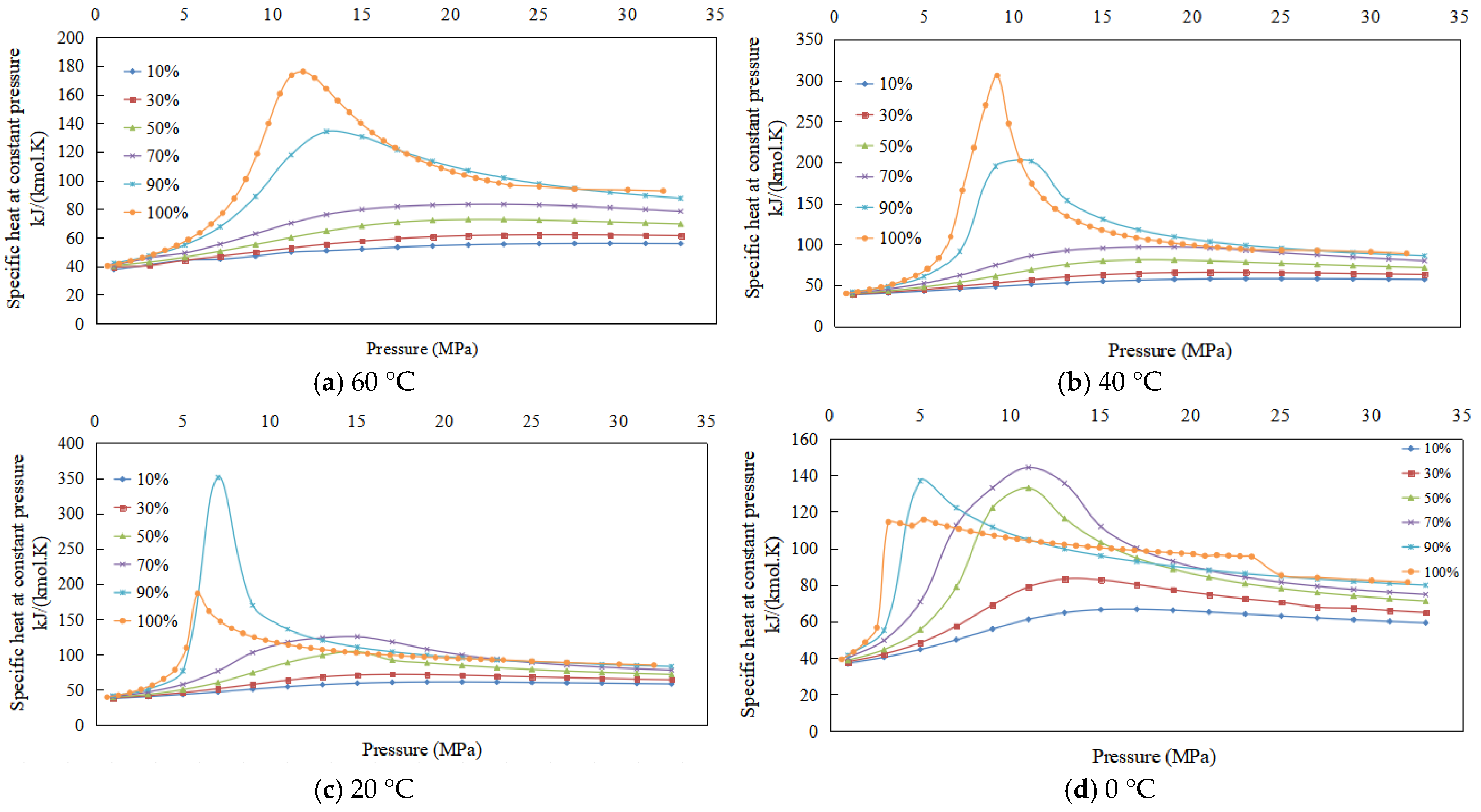
3.5.2. Changes in Specific Heat at Constant Pressure of CO₂ Containing Impurities

(1)

Specific heat at constant pressure increases and then decreases with the increase in pressure.

(2)

The lower the temperature for a given CO₂ content, the specific heat at constant pressure initially increases and subsequently decreases.

(3)

At the same temperature, the higher the CO₂ content, the higher the specific heat at constant pressure under the same pressure; as the temperature decreases, the CO₂ content of the highest specific heat at constant pressure decreases.

4. Calculation and Evaluation of Equations of State

The state equations used most commonly, namely BWRS (Benedict–Webb–Rubin–Starling), PR (Peng–Robinson Equation of State), and SRK (Soave–Redlich–Kwong), are selected. Their characteristics, applicability, and formulas are shown in

Table 4. Characteristics of the equation of state and corresponding formulas.

Equation	Characteristic	Applicability	Formula
BWRS	It is improved from the BWR (Benedict–Webb–Rubin) equation and can accurately describe the PVT characteristics under high pressure and low temperature, which is suitable for calculating CO2 and the density near the critical pressure.	It is applicable to high-purity/high-pressure CO2 systems, acidic gases containing H2S/H2O, and scenarios where the generation of solid CO2 needs to be predicted.	$\begin{array}{l}P=\rho RT+(B_{0}RT-A_0-{\displaystyle \frac{C_0}{T^2}}+{\displaystyle \frac{D_0}{T^3}}-{\displaystyle \frac{E_0}{T^4}}){\rho }^2\\ +(bRT-a-{\displaystyle \frac{d}{T}}){\rho }^3+\alpha (a+{\displaystyle \frac{d}{T}}){\rho }^6\\ +{\displaystyle \frac{c{\rho }^3}{T^2}}(1+\gamma {\rho }^2){\mathrm{e}}^{-\gamma {\rho }^2}\end{array}$
SRK	The calculation of parameters such as compression factor and heat is relatively accurate, and the calculation accuracy of the physical properties of gaseous CO2 is relatively high.	It is suitable for medium and low-pressure hydrocarbon mixtures, scenarios with relatively low CO2 concentration (<30%), and no strong polar impurities.	$P={\displaystyle \frac{RT}{v-b_1}}-{\displaystyle \frac{a_1{\alpha }_1}{v^2+b_{1}v}}$
PR	It is improved from the Clapeyron equation and has high accuracy in the calculation of gas-liquid phase equilibrium and physical properties of polar systems such as CO2.	It is suitable for CO2-hydrocarbon mixed systems, medium-and high-pressure processes (<15 MPa), and scenarios where a balance between precision and speed is required.	$P={\displaystyle \frac{RT}{V_m-b_2}}-{\displaystyle \frac{a_2}{V_m^2+2b_2{V_m-b_2}^2}}$

.

In the formula, P represents the system pressure, kPa. R represents the gas constant, which is taken as 8.3143 J/(mol·K); T represents the gas temperature, K. In the BWRS equation, $\rho$ represents the molar density of the gas, kmol/m³. A₀, B₀, C₀, D₀, a, b, c, d, $\alpha$, and $\gamma$ represent the parameters in the BWRS equation. In the SRK equation, v represents molar volume, m³/mol; a₁, b₁, and ${\alpha }_1$ are related to the critical parameters and eccentricity factor of the fluid. In the PR equation, V_m represents the specific volume of the fluid, m³/mol. a₂ and b₂ are related to the critical parameters and eccentricity factor of the fluid.

4.1. Basic Parameters and Error Calculation Methods

The BWRS, SRK, and PR equations of state were employed to calculate the compression factor and density of gas mixtures with a molar composition of 50% CO₂ and 100% CO₂. The results derived from the equation of state are juxtaposed with the experimental findings (the average value of five physical parameter experimental analyses conducted under each boundary condition is taken as the experimental result). The equation of state yielding results nearest to the experimental values is selected for subsequent calculation. The calculated components are presented in Table 3.

The relative error is used to conduct a comparative analysis of the calculated values of each physical parameter formula and the experimental results, thereby quantifying the calculation accuracy of the three physical equations. The relative error of a single sample point is the difference between the calculated value and the average of the experimental values divided by the average of the experimental values. The specific calculation formula is as follows:

$$\delta ={\displaystyle \frac{x_p-\overline{x}}{\overline{x}}}$$

(1)

where $\delta$ is the relative error, x_p is the physical parameter calculated by the physical equation, and $\overline{x}$ is the experimental average value corresponding to this physical parameter.

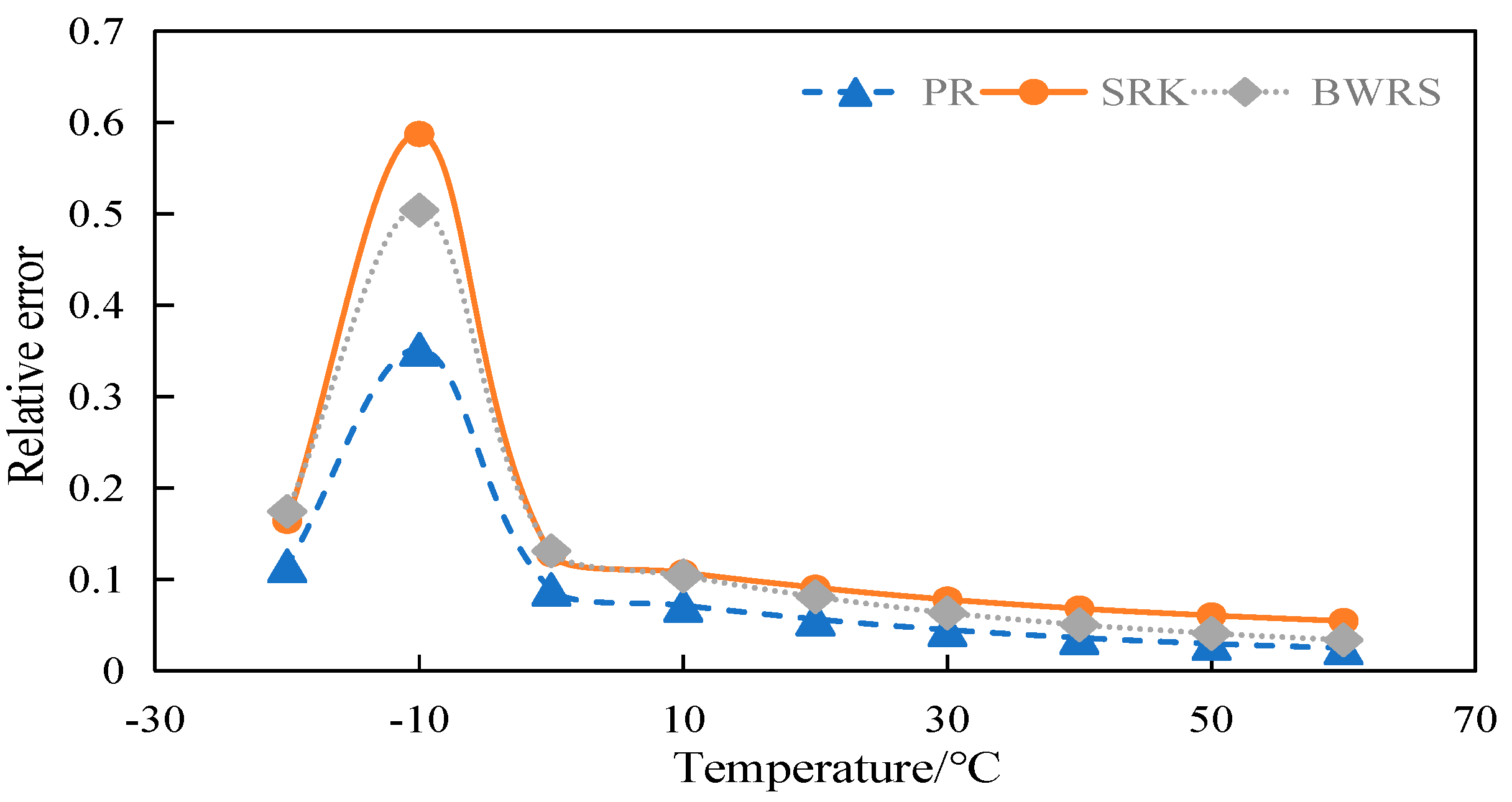
4.2. Compression Factor Calculation

The BWRS, PR, and SRK equations of state were utilized to calculate the compression factor of gas mixtures with a molar composition of 50% and 100% CO₂. The results obtained using each equation of state are compared with the experimental results at different temperatures as follows:

4.2.1. Calculation and Evaluation of Compression Factor of 50% CO₂

The relative error between the compression factor of 50% CO₂ calculated by different equations of state and the experimental results at different temperatures is shown in Figure 7:

With a molar composition of 50% CO₂, the relative errors are 2.28~9.58%, 34.45~67.51%, and 5.21~14.82%, respectively, when calculating the compression factor using the PR, SRK, and BWRS equations of state.

4.2.2. Calculation and Evaluation of Compression Factor of 100% CO₂

The relative errors between the compression factor of 100% CO₂ calculated by different equations of state and the experimental results at different temperatures are shown in Figure 8:

With a molar composition of 100% CO₂, the relative errors are 34.04~57.54%, 34.45~67.51%, and 32.05~65.37%, respectively, when calculating the compression factor using the PR, SRK, and BWRS equations of state.

4.3. Density Calculation

4.3.1. Calculation and Evaluation of Density of 50% CO₂

The relative errors between the density of 50% CO₂ calculated by different equations of state and the experimental results at different temperatures are shown in Figure 9:

With a molar composition of 50% CO₂, the relative errors of density are 2.47~35.19%, 5.44~58.71%, and 3.37~50.40%, respectively, when calculating the density through the PR, SRK, and BWRS equations of state.

4.3.2. Calculation and Evaluation of Density of 100% CO₂

The relative errors between the density of 100% CO₂ calculated by different equations of state and the experimental results at different temperatures are illustrated in Figure 10:

With a molar composition of 10% CO₂, the relative errors of density are 2.82~9.72%, 11.15~18.15%, and 11.15~18.15%, respectively, when calculating the density through the PR, SRK, and BWRS equations of state.

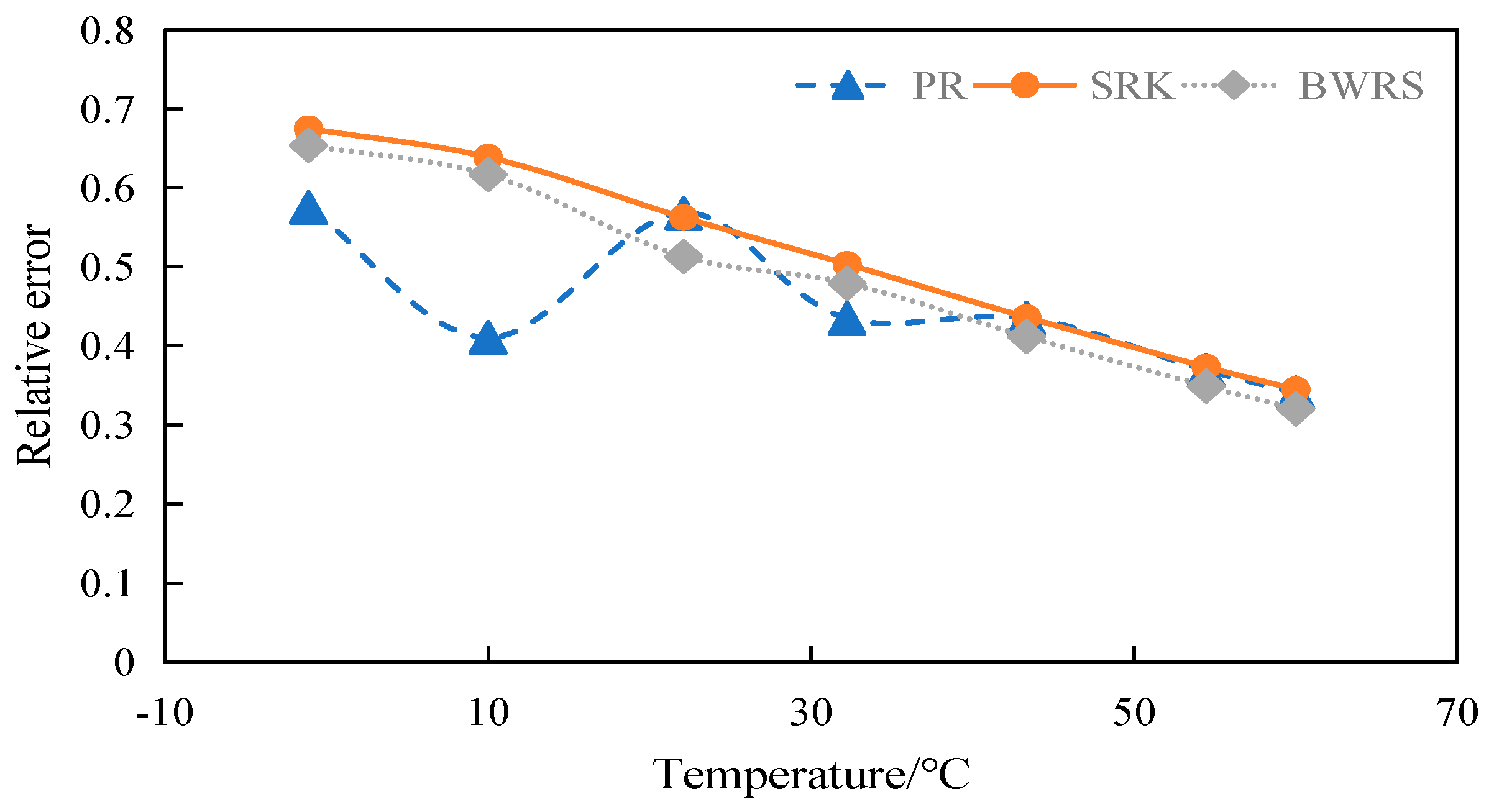
4.4. Viscosity Calculation

The BWRS, PR, and SRK equations of state were leveraged to compute the viscosity of gas mixtures with a molar composition of 50% CO₂ and 100% CO₂. The results derived from each equation of state are compared with the experimental results at different temperatures as follows:

4.4.1. Calculation and Evaluation of Viscosity of 50% CO₂

The relative errors between the viscosity of 50% CO₂ calculated by different equations of state and the experimental results at different temperatures are shown in Figure 11:

When the molar composition of CO₂ is 50%, the average errors of viscosity are 0.50~9.32% when calculating the viscosity through the BWRS equation of state, while the PR and SRK equations of state demonstrate similar errors, averaging between 6.48% and 25.25%. Additionally, the calculation accuracy is higher in the temperature range of 0~50 °C.

4.4.2. Calculation and Evaluation of Viscosity of 100% CO₂

The relative errors between the viscosity of 100% CO₂ calculated by different equations of state and the experimental results across different temperatures are shown in Figure 12:

When the molar composition of CO₂ is 100%, the calculated results of the PR and SRK equations of state are close to the experimental results. Their calculation accuracy surpasses that of the BWRS equation of state at the temperature range of −1.11 °C~54.44 °C. Once the temperature exceeds 54.44 °C, the calculation accuracy of the BWRS equation of state is higher. At temperatures ranging from −1.11 °C to 54.44 °C, the average calculation errors of the PR and SRK equations of state range from 4.06% to 13.28%, while the calculation error of the BWRS equation of state varies between 6.37% and 33.77%. However, with the increase in temperature, the calculation errors of the PR and SRK equations of state escalate significantly, whereas the calculation error of BWRS diminishes at 60 °C.

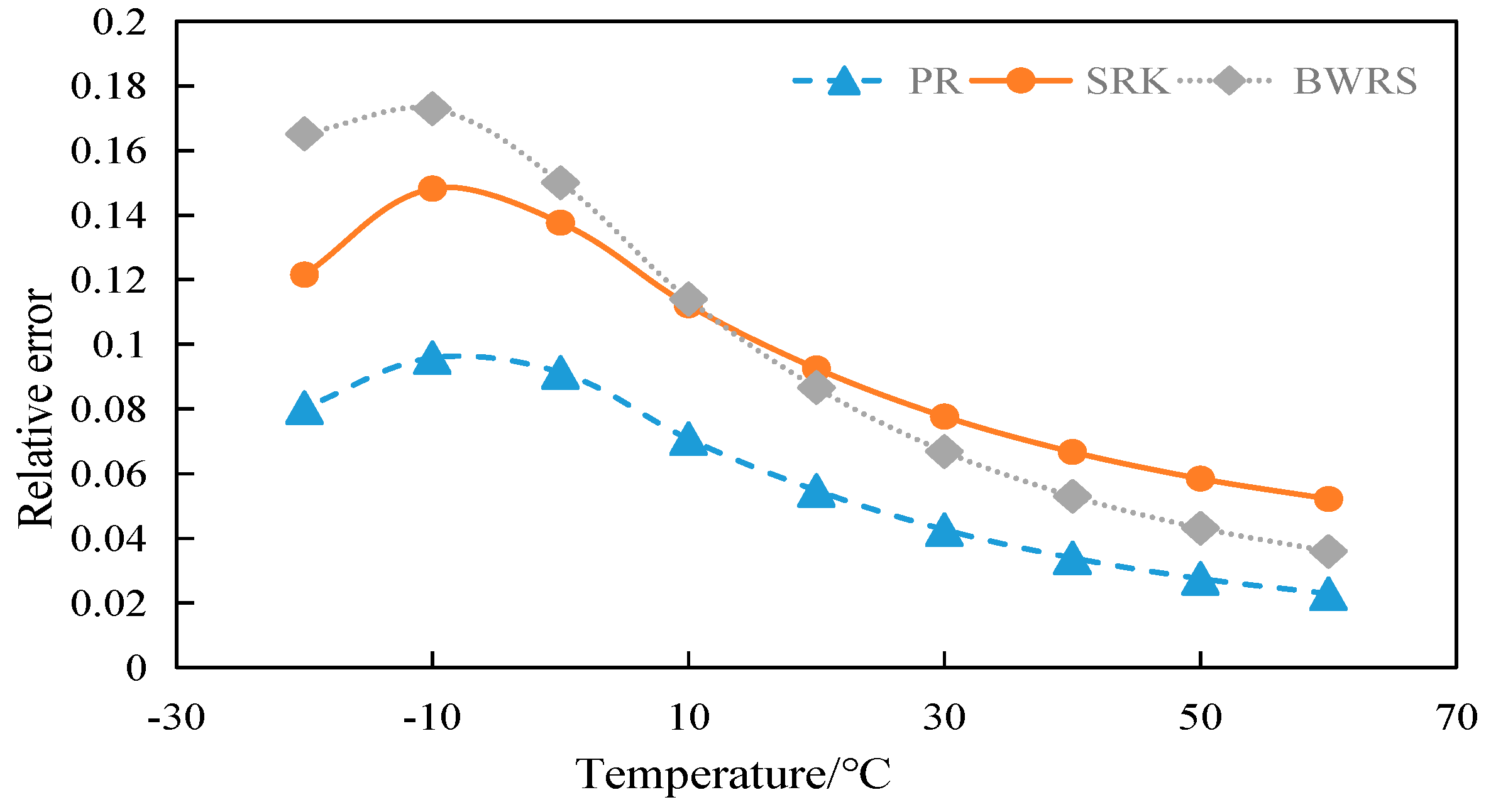
4.5. Calculation of Specific Heat at Constant Pressure

4.5.1. Calculation and Evaluation of Specific Heat at Constant Pressure of 50% CO₂

When the molar composition of CO₂ is 50%, the relative errors between the specific heat at constant pressure calculated by several equations of state and the experimental results at different temperatures are shown in Figure 13:

When the molar composition of CO₂ is 50%, the relative errors of the SRK equation of state vary between 0.53% and 3.15%. The calculation error of the PR equation of state is marginally greater than that of the SRK equation of state, with an average relative error range of 1.26~4.43%. The BWRS equation of state has the lowest calculation accuracy, with an average relative error range of 1.41~1.37%. The calculation error is the largest in the low-temperature zone, and the calculation error decreases progressively with rising temperature.

4.5.2. Calculation and Evaluation of Specific Heat at Constant Pressure of 100% CO₂

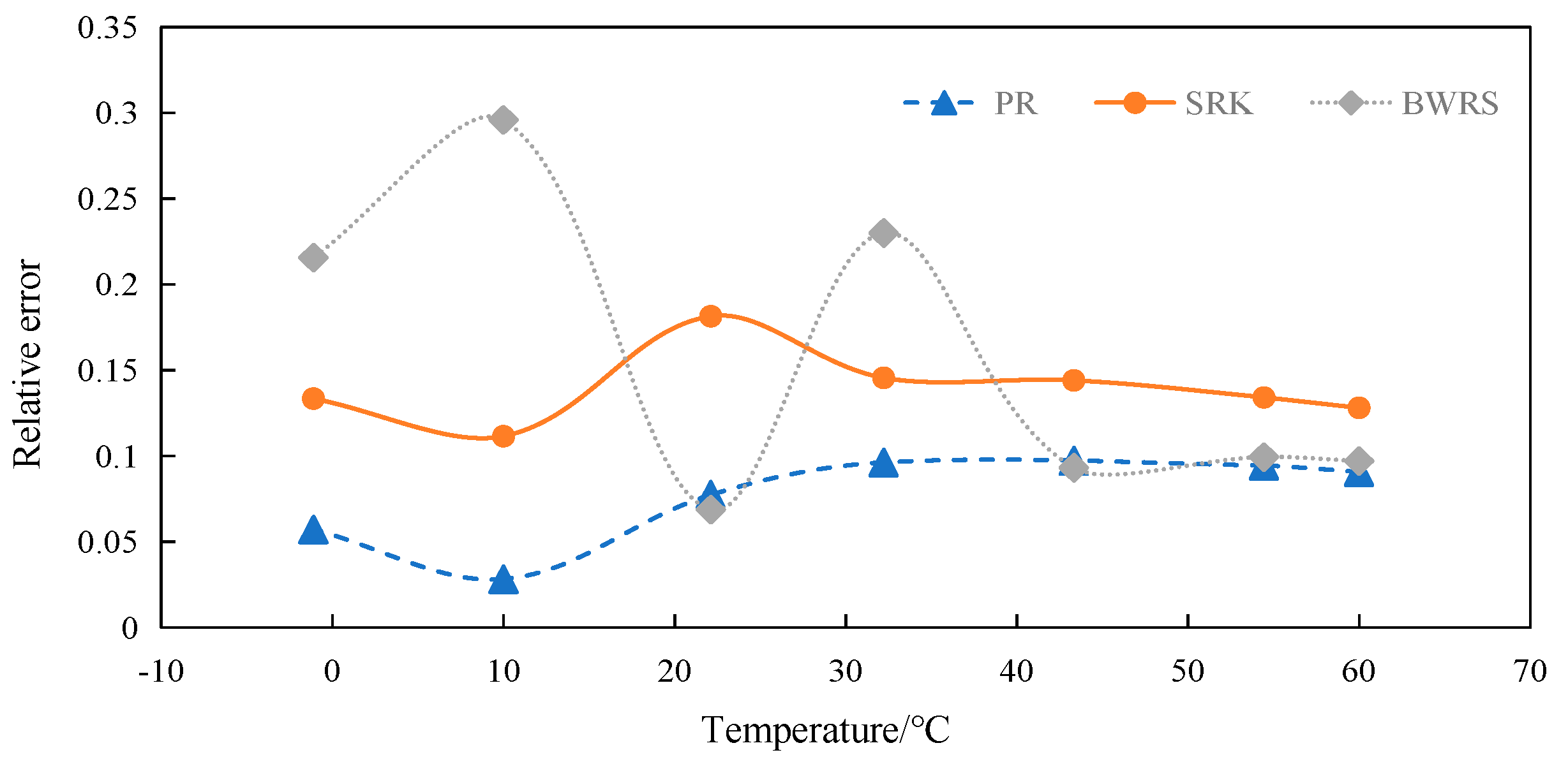
The relative errors between the specific heat at constant pressure of 100% CO₂ calculated by different equations of state and the experimental results at various temperatures are seen in Figure 14.

When the molar composition of CO₂ is 100%, the relative errors of the SRK equation of state vary between 6.31% and 16.91%. The average relative error of the PR equation of state ranges from 6.74% to 17.36%. At low-temperature and high-pressure conditions, the calculated results of the BWRS equation of state are abnormal. The main reason for the anomaly might be that the BWRS equation is close to the pseudo-critical point of the mixture at low temperature and high pressure, and the error of the specific heat at constant pressure in the CO₂ critical zone is greater than 50% [28]. In addition, the 11 parameters of BWRS are usually fitted based on medium- and low-pressure experimental data. In the unfitted low-temperature and high-pressure zone, the parameter combination may cause the function related to the specific heat at constant pressure to lose its physical significance. Excluding the abnormal calculation points, the average relative error range is 4.77~16.25%.

4.6. Summary

(1)

Error between compression factor and experimental data

The PR, BWRS, and SRK equations of state were utilized to calculate the error between the compression factor and the experimental data at different temperatures. The findings indicate that when the molar composition of CO₂ is either 50% or 100%, the calculated results of the PR equation of state closely align with the experimental results.

In addition, the relative errors in the calculated results of the PR, BWRS, and SRK equations of state diminish as temperature rises. The relative error of the calculated results for the 50% CO₂ molar composition is minimal when compared to the 100% CO₂ molar composition.

(2)

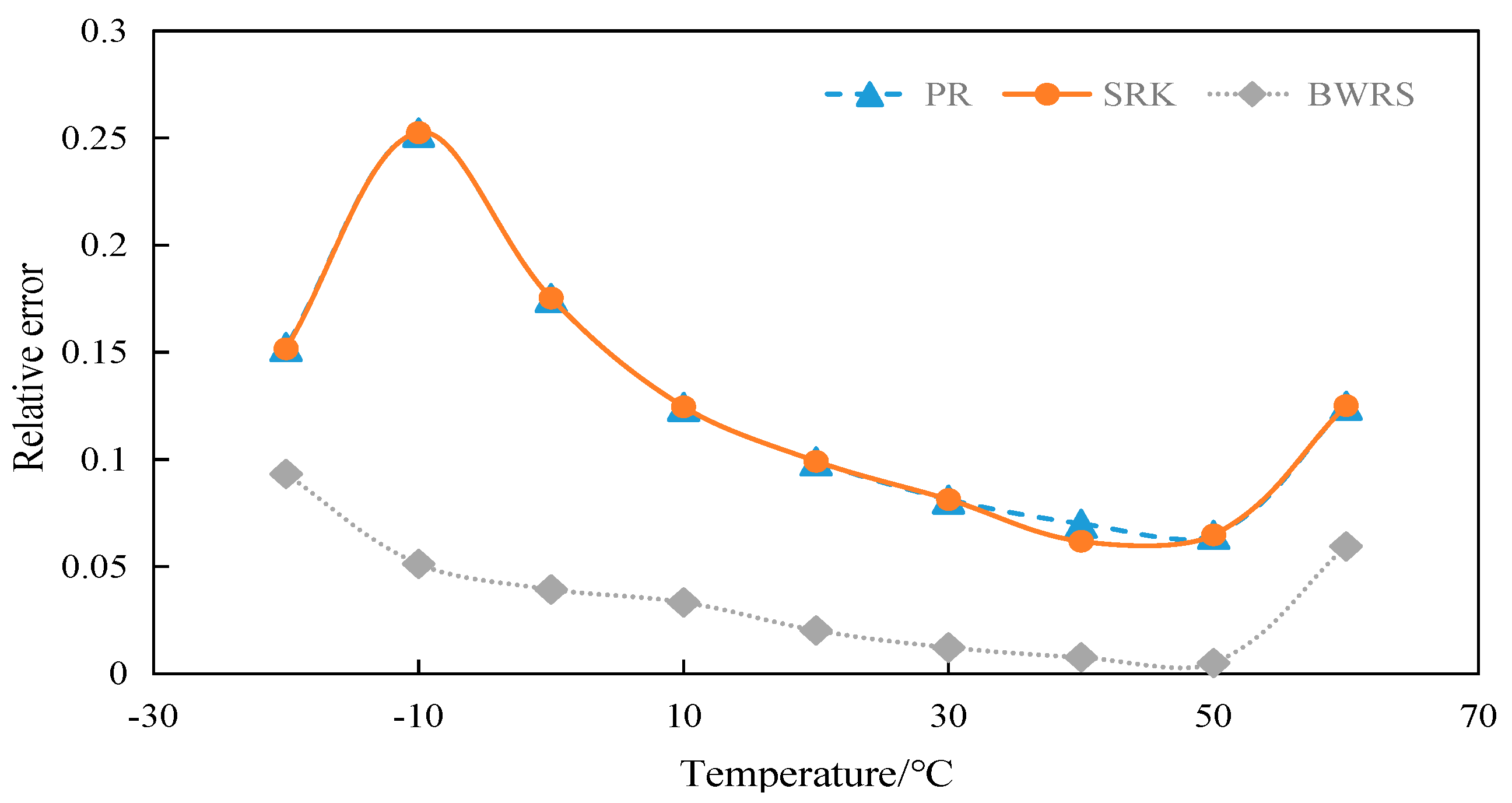
Error between density and experimental data

The PR, BWRS, and SRK equations of state were applied to calculate the error between the density and the experimental data at different temperatures. The findings demonstrate that the relative error of the calculated results of the PR equation of state is minimum when the molar composition of CO₂ is either 50% or 100%.

(3)

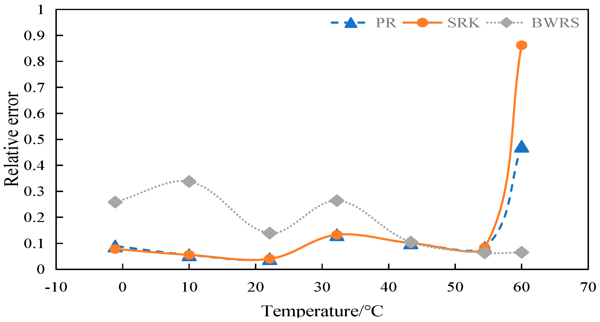
Error between viscosity and experimental data

The PR, BWRS, and SRK equations of state were applied to determine the relative errors between viscosity and experimental data across different temperatures. The findings show that the calculated result of the BWRS equation of state is enhanced when the molar composition of CO₂ is 50%. When the molar composition of CO₂ is 100%, the calculated results of the PR and SRK equations of state closely align with the experimental results.

When the molar composition of CO₂ is 50% or 100%, the calculation error increases rapidly once the calculation temperature exceeds 50 °C.

(4)

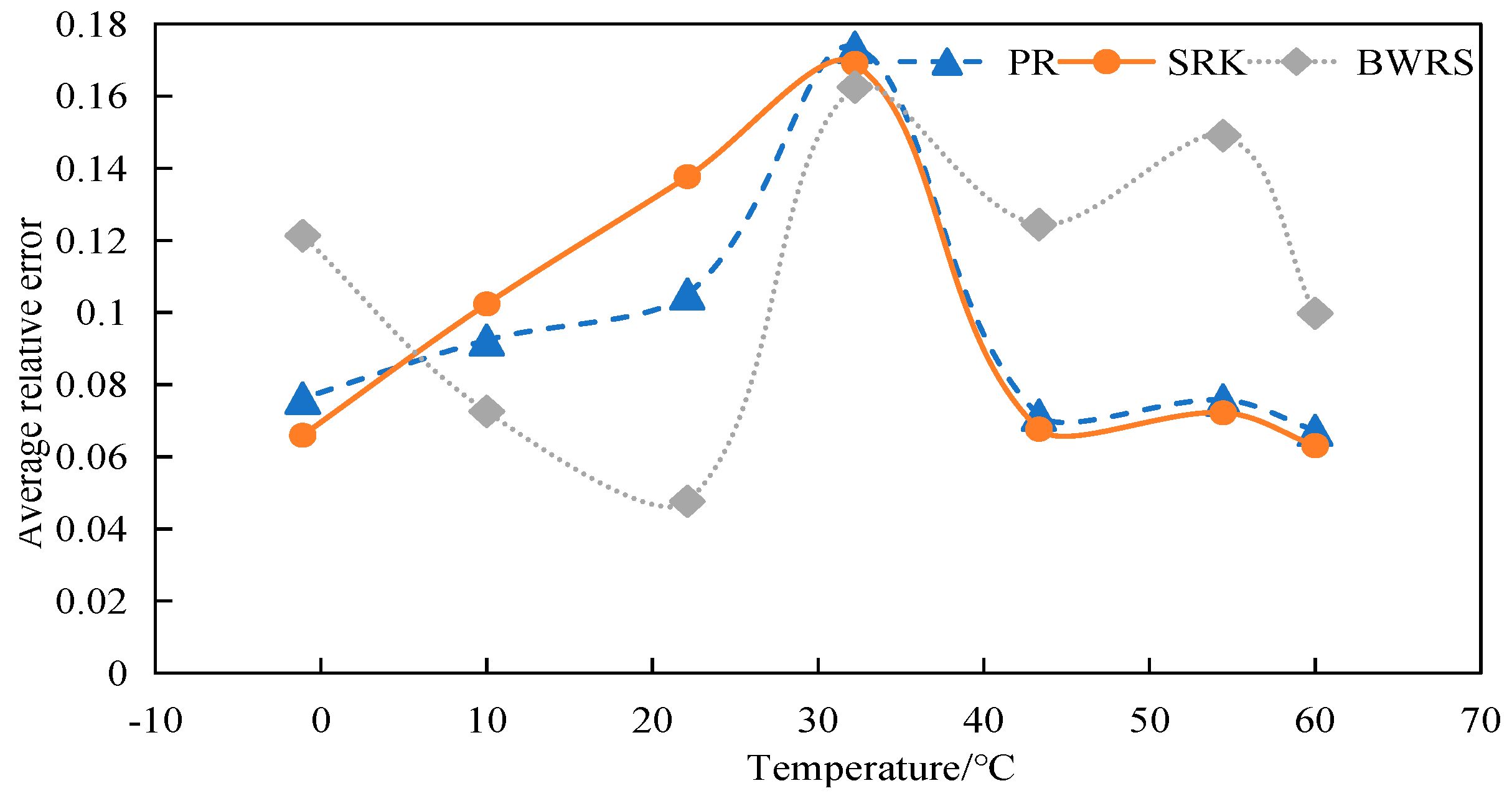
Error between specific heat at constant pressure and experimental data

The PR, BWRS, and SRK equations of state are applied to calculate the relative errors between the specific heat at constant pressure and the experimental data at different temperatures. The findings suggest that the calculated result of the SRK equation of state is more accurate when the molar composition of CO₂ is 50%. However, the calculation accuracy of the PR equation of state is close to that of the SRK equation of state.

(5)

Results summary

When calculating the compression factor, density, and specific heat at constant pressure, the results obtained through the PR state equation are closest to the experimental values, and its accuracy increases with the rise in temperature. As for viscosity calculation, the calculated result of the BWRS equation of state is the closest to the experimental value when the molar composition of CO₂ is 50%. However, when the molar composition of CO₂ reaches 100%, the calculation error of the PR equation of state is equivalent to that of the SRK equation of state. Consequently, the PR equation of state is selected for calculating CO₂-related physical property parameters, based on extensive analysis and comparison.

The physical property parameters of a CO₂ mixed system are determined through experiment and literature review. Upon comparing such physical property parameters with the results calculated by the PR, SRK, and BWRS equations of state, the following conclusions can be drawn in

Table 5. Calculation error range of each equation of state and recommended equations of state.

Composition	Calculation Parameters	PR/%	SRK/%	BWRS/%	Recommended Equations of State
50% CO2	Compression factor	2.28~9.58	34.45~67.51	5.21~14.82	PR
50% CO2	Density	2.47~35.19	5.44~58.71	3.37~50.40	PR
50% CO2	Viscosity	6.48~25.25	6.48~25.25	0.50~9.32	BWRS
50% CO2	Specific heat at constant pressure	1.26~4.43	0.53~3.15	1.41~11.37	PR
100% CO2	Compression factor	34.04~57.54	34.45~67.51	32.05~65.37	PR
100% CO2	Density	2.82~9.72	11.15~18.15	6.88~29.59	PR
100% CO2	Viscosity	4.06~13.28	4.06~13.28	6.37~33.77	PR
100% CO2	Specific heat at constant pressure	6.74~17.36	6.31~16.91	4.77~25.86	SRK

:

From the above table and the above analysis, it can be known that in pure CO₂ and CO₂ multi-component systems, when the compression factor, density, and specific heat at constant pressure are comprehensively calculated, the results obtained through the PR state equation are the closest to the experimental values.

5. Conclusions

Through experiments on the physical property parameters of carbon dioxide containing impurities and in combination with the three state equations of PR, SRK, and BWRS for the calculation of physical parameters such as compression factor, density, and specific heat at constant pressure, the following conclusions are drawn:

(1)

The compression factor first decreases and then increases with the increase in pressure, and the lower the temperature, the smaller the critical compression factor. At the same temperature, the higher the CO₂ content, the smaller the compression factor under the same pressure. Density and viscosity increase with the rise in pressure, and the lower the temperature, the higher the corresponding density and viscosity. At the same temperature, the higher the CO₂ content, the higher the density and viscosity under the same pressure. The specific heat at constant pressure increases first and then decreases with the increase in pressure, and the lower the temperature, the specific heat at constant pressure increases first and then decreases. At the same temperature, the higher the CO₂ content, the higher the specific heat at the same pressure.

(2)

The BWRS equation of state shows great accuracy fluctuation in physical property parameter calculations. Under lower temperature conditions, a substantial error will arise between the calculated values and the experimental values. Conversely, the equation demonstrates higher-accuracy calculation within the elevated temperature range. Nevertheless, such an elevated temperature range is infrequently reached in real-world isothermal transportation. Furthermore, the BWRS equation is characterized by mass coefficients, which complicates the calculation procedure. Consequently, it is inadvisable to apply this equation while exploring the characteristics of multi-component CO₂ in pipeline transport.

(3)

The SRK equation of state exhibits consistent calculation results. However, the predicted value is lower than the experimental value. There is a large deviation from the actual density value of CO₂ in the conventional temperature range of pipeline transport.

(4)

The PR equation features accurate simulation calculations and straightforward calculation procedures, and its calculation results closely align with the experimental values. It is recommended to use the PR equation of state in the pipeline transport of CO₂.

(5)

Based on the investigation of the influence mechanism of carbon dioxide containing impurities, it is concluded that when H₂S/H₂O impurities are present, the built-in polarity correction term of BWRS makes the calculation more stable. When the temperature is less than 40 °C and it is necessary to predict the freezing point of CO₂ or the formation of hydrates, BWRS can describe the solid-phase equilibrium. When supercritical CO₂ extraction is carried out, the accuracy of BWRS is significantly better than that of the PR and SRK equations.

References

1. IPCC. Carbon Dioxide Capture and Storage; Cambridge University Press: New York, NY, USA, 2005. [Google Scholar]
2. Czernichowski-Lauriol, I.; Berenblyum, R.; Bigi, S.; Car, M.; Gastine, M.; Persoglia, S.; Poulsen, N.; Schmidt-Hattenberger, C.; Stead, R.; Vincent, C.J.; et al. CO2 GeoNet actions in Europe for advancing CCUS through global cooperation. Energy Procedia 2018, 154, 73–79. [Google Scholar] [CrossRef]
3. Bhave, A.; Taylor, R.H.; Fennell, P.; Livingston, W.R.; Shah, N.; Mac Dowell, N.; Dennis, J.; Kraft, M.; Pourkashanian, M.; Insa, M.; et al. Screening and techno-economic assessment of biomass-based power generation with CCS technologies to meet 2050 CO2 targets. Appl. Energy 2017, 190, 481–489. [Google Scholar] [CrossRef]
4. Reiner, D.M. Learning through a portfolio of carbon capture and storage demonstration projects. Nat. Energy 2016, 1, 15011. [Google Scholar] [CrossRef]
5. Lilliestam, J.; Bielicki, J.M.; Patt, A.G. Comparing carbon capture and storage (CCS) with concentrating solar power (CSP): Potentials, costs, risks, and barriers. Energy Policy 2012, 47, 447–455. [Google Scholar] [CrossRef]
6. Gale, J.; Davison, J. Transmission of CO2—Safety and economic considerations. Energy 2004, 29, 1319–1328. [Google Scholar] [CrossRef]
7. Bears, D.A.; Wied, R.F.; Martin, A.D.; Doyle, R.P. Paradis CO2 flood gathering, injection, and production systems. J. Pet. Technol. 1984, 36, 1312–1320. [Google Scholar] [CrossRef]
8. Kleinstelber, S.W. The Wertz Tensleep CO2 flood: Design and initial performance. J. Pet. Technol. 1990, 42, 630–636. [Google Scholar] [CrossRef]
9. Wilson, A. CO2 enhanced-oil-recovery project injects new life into Madison Reservoir in Wyoming. J. Pet. Technol. 2012, 64, 112–115. [Google Scholar] [CrossRef]
10. Brown, S.; Martynov, S.; Mahgerefteh, H.; Fairweather, M.; Woolley, R.M.; Wareing, C.J.; Falle, S.A.; Rutters, H.; Niemi, A.; Zhang, Y.C.; et al. CO2QUEST: Techno-economic assessment of CO2 quality effect on its storage and transport. Energy Procedia 2014, 63, 2622–2629. [Google Scholar] [CrossRef]
11. Mohitpour, M.; Seevam, P.; Botros, K.K.; Rothwell, B.; Ennis, C. Pipeline Transportation of Carbon Dioxide Containing Impurities; ASME Press: New York, NY, USA, 2012. [Google Scholar]
12. Nezhad, S.; Williams, C. Bravo Dome Subsurface and Surface Network Modeling. In Proceedings of the Abu Dhabi International Petroleum Exhibition and Conference, Abu Dhabi, United Arab Emirates, 10–13 November 2014. [Google Scholar]
13. Jung, W.; Nicot, J.P. Impurities in CO2-rich mixtures impact CO2 pipeline design: Implications for calculating CO2 transport capacity. In Proceedings of the SPE International Conference on CO2 Capture, Storage, and Utilization, New Orleans, LA, USA, 10–12 November 2010. SPE-139712-MS. [Google Scholar]
14. McCollough, D.E.; Stiles, R.L. Operation of the Central Basin CO2 pipeline system. In Proceedings of the SPE Western Regional Meeting, Ventura, CA, USA, 8–10 April 1987. SPE-16329-MS. [Google Scholar]
15. Towler, B.F.; Agarwal, D.; Mokhatab, S. Modeling Wyoming’s carbon dioxide pipeline network. Energy Sources Part A Recovery Util. Environ. Eff. 2007, 30, 259–270. [Google Scholar] [CrossRef]
16. De Nier, M.; Maas, W.; Gray, L.; Wiwchar, T. Maturing CCS Technology through Demonstration Quest: Learning from CCS Implementation in Canada. In Proceedings of the Abu Dhabi International Petroleum Exhibition and Conference, Abu Dhabi, United Arab Emirates, 9–12 November 2015. [Google Scholar]
17. IEA. Energy Technology Perspectives 2020; IEA: Paris, France, 2020. [Google Scholar]
18. Edward, S.R.; John, E.D.; Howard, J.H. The cost of CO2 capture and storage. Int. J. Greenh. Gas Control. 2015, 40, 378–400. [Google Scholar] [CrossRef]
19. Government of the United Kingdom. Re-Use of Oil and Gas Assets for Carbon Capture Usage and Storage Projects; Government of the United Kingdom: London, UK, 2019.
20. Lone, S.; Cockerill, T.; Macchietto, S. The techno-economics of a phased approach to developing a UK carbon dioxide pipeline network. J. Pipeline Eng. 2010, 9, 223. [Google Scholar]
21. Sandana, D.; Dale, M.; Charles, E.; Race, J. Transport of gaseous and dense carbon dioxide in pipelines: Is there an internal corrosion risk. J. Pipeline Eng. 2012, 11, 229–238. [Google Scholar]
22. Choi, Y.S.; Nesic, S.; Young, D. Effect of impurities on the corrosion behavior of CO2 transmission pipeline steel in supercritical CO2-water environments. Environ. Sci. Technol. 2010, 44, 9233–9238. [Google Scholar] [CrossRef] [PubMed]
23. Sim, S.; Cole, I.S.; Bocher, F.; Corrigan, P.; Gamage, R.P.; Ukwattage, N.; Birbilis, N. Investigating the effect of salt and acid impurities in supercritical CO2 as relevant to the corrosion of carbon capture and storage pipelines. Int. J. Greenh. Gas Control 2013, 17, 534–541. [Google Scholar] [CrossRef]
24. Froydis, E. Safe pipeline transmission of CO2. Pipeline Gas J. 2008, 235, 76–77. [Google Scholar]
25. Zhang, Z.; Pan, S.Y.; Li, H. Recent Advances in Carbon Dioxide Utilization. Renew. Sustain. Energy Rev. 2020, 125, 109799. [Google Scholar] [CrossRef]
26. Munkejord, S.T.; Austegard, A.; Deng, H.; Hammer, M.; Stang, H.J.; Løvseth, S.W. Depressurization of CO2 in a pipe: High-resolution pressure and temperature data and comparison with model predictions. Energy 2020, 211, 118560. [Google Scholar] [CrossRef]
27. Vanchugov, I.M.; Rezanov, K.S.; Shestakov, R.A. On the issue of transportation of liquefied carbon dioxide. Bull. Tomsk. Polytech. Univ. Geo Assets Eng. 2023, 334, 190–209. [Google Scholar] [CrossRef]
28. Span, R.; Wagner, W. A new equation of state for carbon dioxide covering the fluid region from the triple-point temperature to 1100 K at pressures up to 800 MPa. J. Phys. Chem. Ref. Data 1996, 25, 1509–1596. [Google Scholar] [CrossRef]
29. Fenghour, A.; Wakeham, W.A.; Vesovic, V. The viscosity of carbon dioxide. J. Phys. Chem. Ref. Data 1996, 25, 1599–1610. [Google Scholar] [CrossRef]
30. Kontogeorgis, G.M.; Folas, G.K. Thermodynamic Models for Industrial Applications: From Classical and Advanced Mixing Rules to Association Theories; John Wiley & Sons: Hoboken, NJ, USA, 2010. [Google Scholar]
31. Li, H.; Jakobsen, J.P. PVTxy properties of CO2 mixtures relevant for CO2 capture, transport and storage: Review of available experimental data and theoretical models. Appl. Energy 2013, 111, 815–826. [Google Scholar] [CrossRef]
32. Gernert, G.J.; Span, R. EOS-CG: A Helmholtz energy mixture model for humid gases and CCS mixtures. J. Chem. Thermodyn. 2016, 93, 274–293. [Google Scholar] [CrossRef]
33. Ahmadi, P.; Chapoy, A. Experimental and modelling studies on the phase behaviour of (CO2+H2S) binary and (CO2+H2S+CH4) ternary systems. J. Chem. Thermodyn. 2017, 115, 127–138. [Google Scholar]
34. ISO 20486:2017; Petroleum and Natural Gas Industries—Fluid Properties—Determination of Reservoir Fluid Properties by Laboratory Analysis. International Organization for Standardization: Geneva, Switzerland, 2017.
Figure 1. Flowchart of the natural gas PVT experimental test.
Fluids 10 00189 g001
Figure 2. DBR-JEFRI mercury-free high-temperature and high-pressure formation fluid analyzer.
Fluids 10 00189 g002
Figure 3. Pressure-dependent compression factor changes for different CO2 content at different temperatures.
Fluids 10 00189 g003
Figure 4. Pressure-dependent density changes for different CO2 content at different temperatures.
Fluids 10 00189 g004
Figure 5. Viscosity changes with pressure for different CO2 content at various temperatures.
Fluids 10 00189 g005
Figure 6. Changes in specific heat at constant pressure with pressure for different CO2 contents at various temperatures.
Fluids 10 00189 g006
Figure 7. Comparison of compression factor calculation results of 50% CO2 at −20~60 °C.
Fluids 10 00189 g007
Figure 8. Comparison of the compression factor calculation results of 100% CO2 at 0 °C.
Fluids 10 00189 g008
Figure 9. Relative errors of density of 50% CO2 at different temperatures.
Fluids 10 00189 g009
Figure 10. Relative errors of density of 100% CO2 at different temperatures.
Fluids 10 00189 g010
Figure 11. Comparison of viscosity calculation results of 50% CO2 at −20~60 °C.
Fluids 10 00189 g011
Figure 12. Comparison of viscosity calculation results of 100% CO2 at 0 °C.
Fluids 10 00189 g012
Figure 13. Relative errors of specific heat at constant pressure of 50% CO2 at different temperatures.
Fluids 10 00189 g013
Figure 14. Relative errors of specific heat at constant pressure of 100% CO2 at different temperatures.
Fluids 10 00189 g014