Abstract
We present a neural-network-based approach to solve the image-to-image translation problem in microscale droplets squeeze flow. A residual convolutional neural network is proposed to address the inverse problem: reconstructing a low-resolution (LR) droplet pattern image from a high-resolution (HR) liquid film thickness imprint. This enables the prediction of initial droplet configurations that evolve into target HR imprints after a specified spreading time. The developed neural network architecture aims at learning to tune the refinement level of its residual convolutional blocks by using function approximators that are trained to map a given film thickness to an appropriate refinement level indicator. We use multiple stacks of convolutional layers, the output of which is translated according to the refinement level indicators provided by the directly connected function approximators. Together with a non-linear activation function, the translation mechanism enables the HR imprint image to be refined sequentially in multiple steps until the target LR droplet pattern image is revealed. We believe that this work holds value for the semiconductor manufacturing and packaging industry. Specifically, it enables desired layouts to be imprinted on a surface by squeezing strategically placed droplets with a blank surface, eliminating the need for customized templates and reducing manufacturing costs. Additionally, this approach has potential applications in data compression and encryption.
1. Introduction
Thin films play a crucial role in numerous natural and industrial processes. Researchers have extensively examined the flow of thin films over both flat and curved surfaces [1,2]. This interest partly stems from their significance in spin coating and photolithography—key steps in manufacturing microelectronic components, integrated circuits, magnetic storage devices, optical devices, and compact disks. Pettas et al. employed finite element simulations to analyze the two-dimensional Navier–Stokes equations, investigating thin-film flow along inclined surfaces with deep microgrooves for both Newtonian [3] and non-Newtonian fluids [4].
Among the diverse types of thin-film flows, squeeze flow has applications across multiple disciplines, including engineering, biology, and rheometry [5]. Examples include elastohydrodynamic lubrication [6], cerebrospinal fluid dynamics in the skull [7], heat-sealing processes [8], viscoelastic fluid characterization using oscillatory squeeze rheometry [9], and resin flow in display manufacturing techniques [10].
The squeeze flow of thin films is particularly important in imprint lithography for filling microscale and nanoscale cavities, trenches, and other features. Different lithography methods, such as plate-to-plate [11], roll-to-plate [12], and roll-to-roll [12,13], rely on this mechanism. Rowland et al. [11] conducted finite element simulations with moving boundaries to analyze thin film embossing in nanoimprint lithography (NIL), seeking to optimize process parameters. Their study examined how cavity geometry, polymer film thickness, material properties, and processing conditions influence polymer deformation and filling rates. They found that shear localization and polymer flow dynamics dictate filling efficiency and proposed three key parameters—cavity width-to-film thickness ratio, polymer supply ratio, and capillary number—to predict deformation modes. These findings provide a framework for optimizing NIL by adjusting geometry, process settings, and material properties.
1.1. Imprint Lithography
Imprint lithography and particularly a subclass of it called step and flash imprint lithography (SFIL) [14] are considered as promising alternatives to the photolithography process. In SFIL, the imprint resist droplets are dispensed on a substrate, followed by squeezing the droplets using a superstrate (template) and curing the resulting liquid film into a desired pattern [14,15]. Inspired by SFIL, herein, we investigate the possibility of producing desired imprint images on a substrate by using a blank superstrate. To the best of our knowledge, for the first time, we attempt to identify an appropriate droplet pattern map that, when squeezed by a blank superstrate, can lead to a given target imprint image, through which the costs associated with the design and manufacture of customized templates can be eliminated.
Let us consider a pair of parallel plates (substrate and superstrate) initially separated from each other as shown in Figure 1.

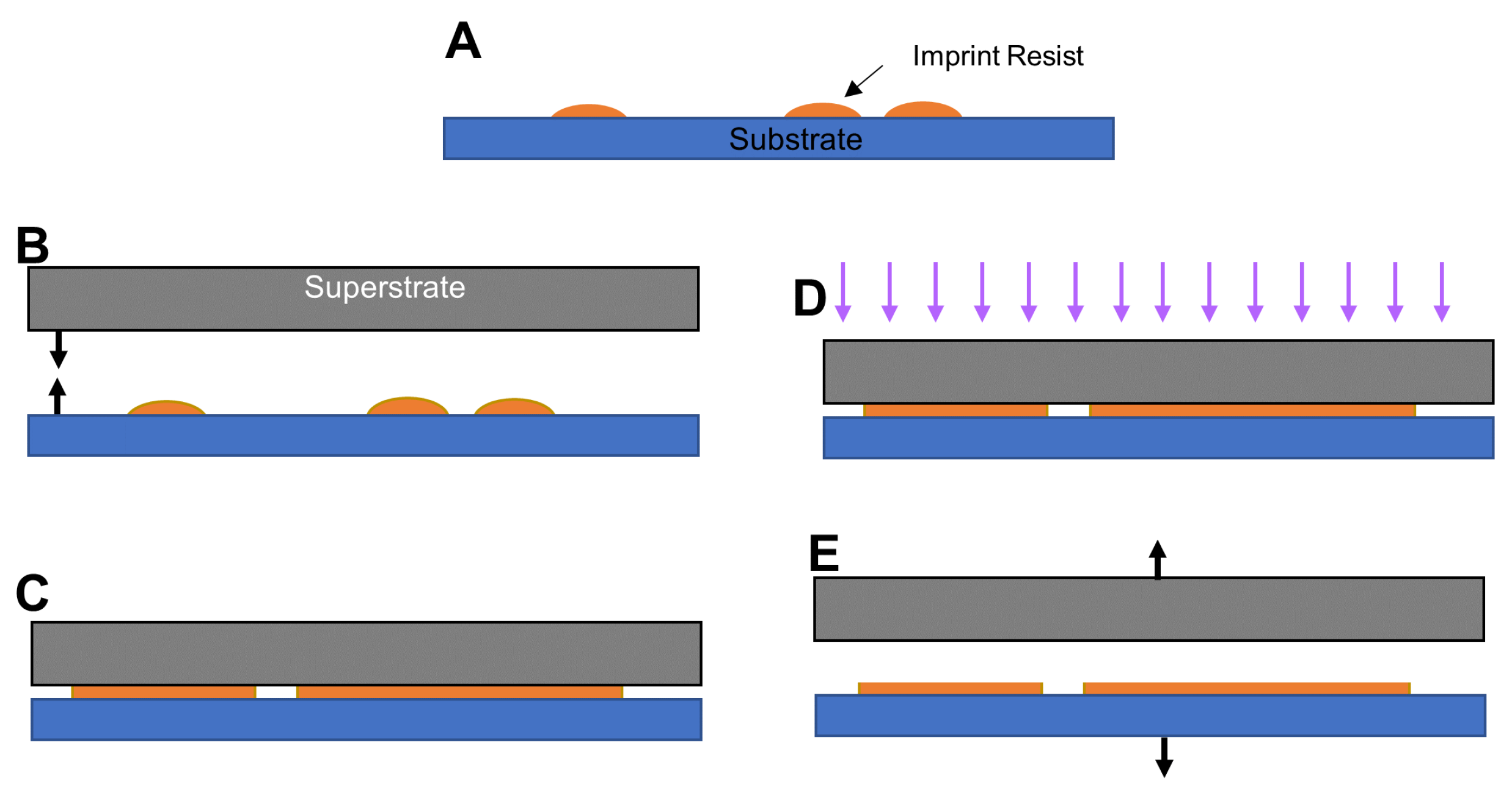
Figure 1.
A schematic representation of the imprint lithography with blank superstrate: (A) dispensing imprint resist droplets according to a droplet pattern, (B) alignment of superstrate (template) and substrate as needed followed by squeezing the droplets, (C) spreading and merging of imprint resist droplets, (D) polymerization of imprint resist using the UV exposure, and (E) separation of template from substrate.
First, one or multiple droplets of imprint resist are dispensed on the substrate using an inkjet dispenser according to a droplet pattern map. The superstrate is then brought into contact with the liquid droplets. Because of the capillary force, the droplets start to spread and merge. The flow of liquid continues for a period of time, the length of which is called spread time. The resulted liquid film is then polymerized by using an ultraviolet (UV) exposure. The superstrate is debonded from the substrate at the end. The main difference between this methodology and SFIL is that, instead of using a customized template, in this work, we consider a blank superstrate aiming at finding the appropriate initial position of droplets that can produce a given pattern with a specific film thickness.
1.2. Droplet Pattern Image and Imprint Image
In practice, an inkjet printhead has an array of nozzles separated by a finite distance, which is typically of the order of tens of microns. The pitch of the nozzle array dictates the pixel size of the droplet pattern image. The droplet pattern image is simply a representation of the firing nozzles. For each nozzle that dispenses a droplet, the corresponding pixel is considered to have the value of ‘1’ (On). Otherwise, a value of ‘0’ (Off) is assigned to the corresponding pixel.
On the other hand, the imprint image is a top-down view of the liquid film. The areas with liquid are assigned a value of ‘1’ (Wet), while a value of ‘0’ is considered for areas without liquid (Dry). We have developed a physics-based model to simulate the squeeze flow of droplets for any given droplet pattern (forward problem). The physical domain of interest is discretized into a finite number of computational cells. Therefore, the pixel size of the imprint image is dictated by the size of the computational cells.
1.3. Forward and Inverse Problems
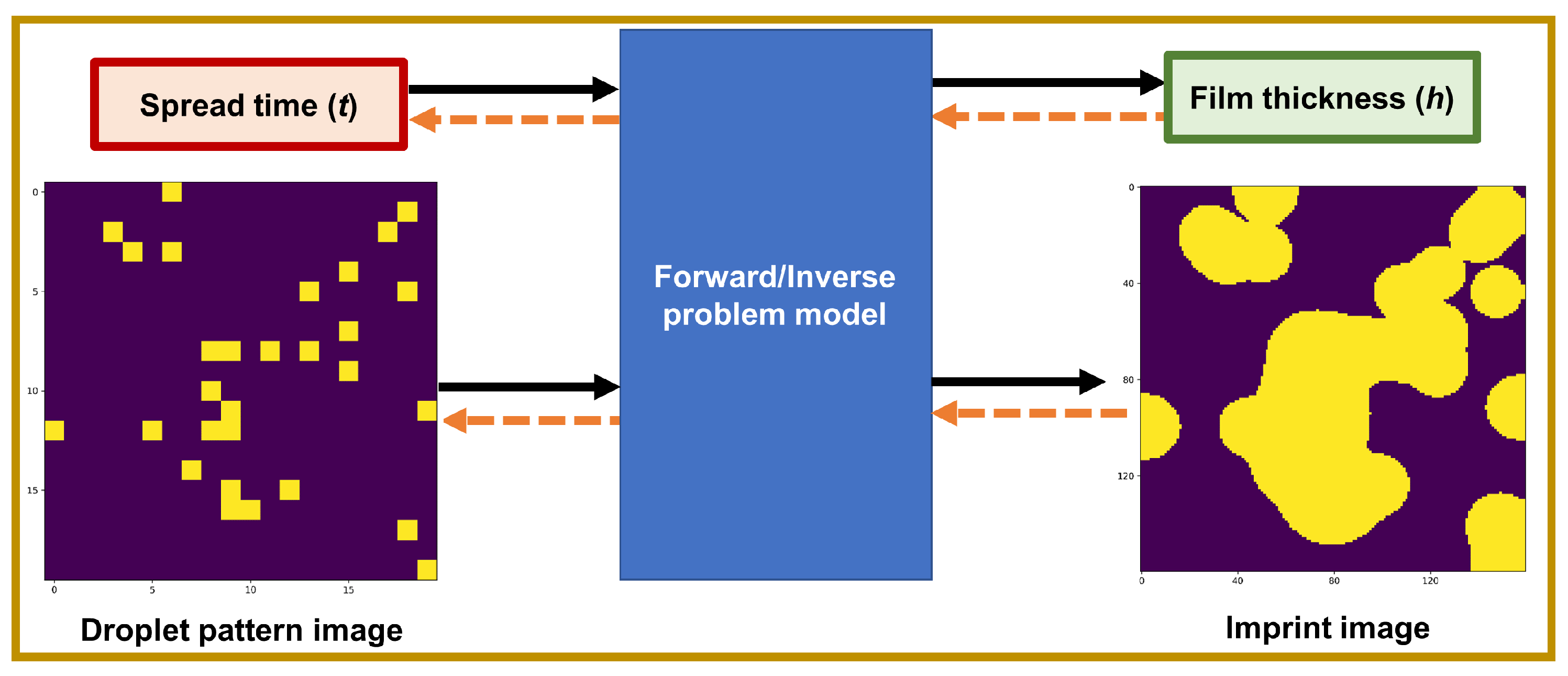
The schematic representation depicted in Figure 2 illustrates the forward and inverse problems of the squeeze flow of droplets.
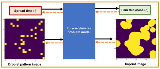
Figure 2.
A general schematic representation of the forward (solid black arrows) and inverse (orange dashed arrows) problems for the squeeze flow of droplets.
Although the forward problem, i.e., the prediction of the 1. imprint image and 2. film thickness from a given tuple of the 1. drop pattern image and 2. spread time, is achievable using a physics-based solver, the inverse problem may not be straightforward; that is, given an imprint image with a specific film thickness, it may not be trivial to find the appropriate drop pattern image and the required spread time.
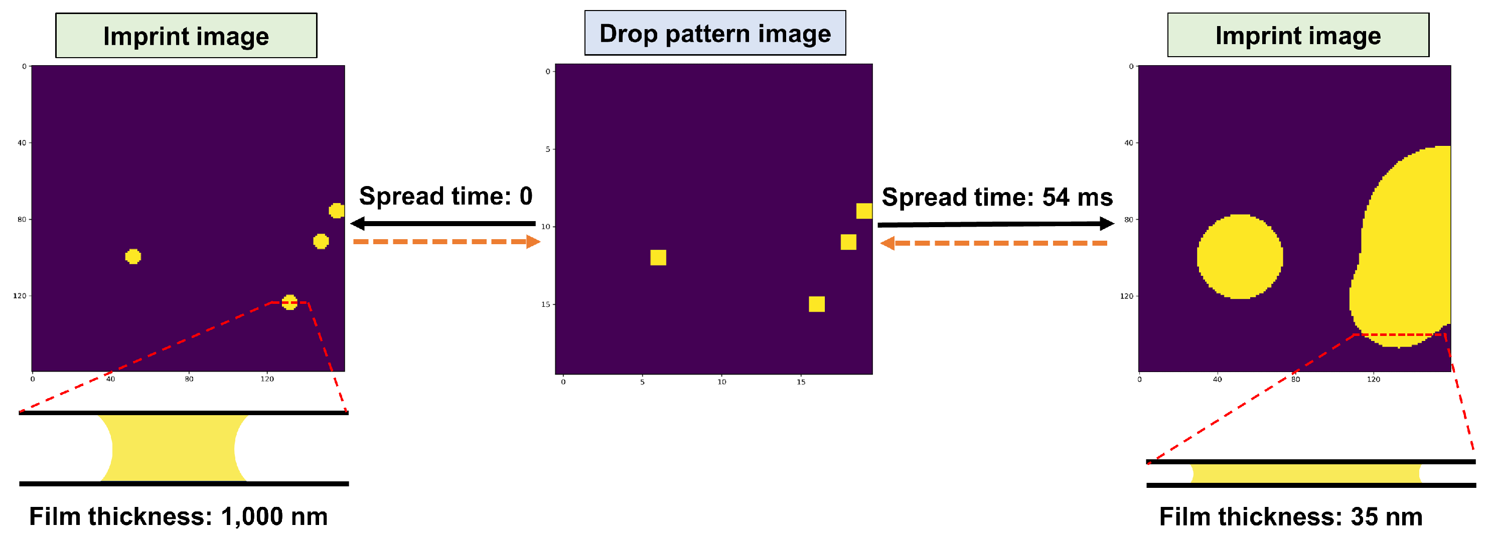
For the example shown in Figure 3, two imprint images are produced with two different film thicknesses for a given drop pattern image under two different spread times.
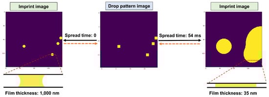
Figure 3.
A droplet pattern image together with the (numerically) produced imprint images for two different spread times as well as the schematic representations of the cross section view of the liquid film. The solid black arrows show the forward problem while the orange dashed arrows denote the inverse problem. Here, the droplet pattern image has pixels while the imprint images consist of pixels. The liquid’s thermophysical properties and other related parameters are discussed in the text.
It can be observed that the droplet pattern map itself can be a good model representation of the imprint image at the beginning of the spread of droplets (after applying an appropriate transformation to resize the image). However, as time elapses, the error associated with such a crude model can become noticeably larger as this basic model ignores the dynamics of squeeze flow and the evolution of liquid film over time.
While we primarily address the inverse problem in this work, the curated dataset can also potentially benefit the community of machine learning and computer vision for testing algorithms on time series images, image-to-image translation [16], multi-class multi-label classifications [17,18,19], image super-resolution [20,21,22,23,24], image deblurring [25,26,27], etc.
1.4. Machine Learning and Fluid Mechanics
Over the last decade, with the enormous growth of hardware capabilities, many applications of machine learning techniques have emerged in the field of fluid mechanics [28,29,30]. Physics-informed machine learning has emerged as an approach integrating data and mathematical physics models [31]. Raissi et al. introduced a new class of universal function approximators called physics-informed neural networks (PINNs) that are capable of encoding any underlying physical laws that govern a given dataset, and can be described by partial differential equations [32]. PINNs use automatic differentiation to represent all the differential operators, and therefore do not rely on a mesh generation. Instead, the Navier–Stokes equations can be incorporated in the loss function of the neural network (NN) by penalizing the deviations from the target values, e.g., zero residuals for the conservation laws. PINNs have been used widely to solve forward and inverse problems in fluid mechanics [33,34,35], solid mechanics [36], and heat transfer [37], among other applications. PINNs, however, do not replace the existing computational fluid dynamics (CFD) methods, and are known to be less accurate than high-order CFD techniques [38].
In this work, we use a supervised learning approach, wherein the forward problem is solved using a physics-based solver to curate a large dataset. The dataset is then used to train a neural network capable of solving the inverse problem. The developed model provides a computationally efficient approach for large-scale systems, eliminating the need for complex forward problem modeling (of many systems) when solving inverse problems.
2. Methodology
2.1. Physics-Based Solver
In this section, we discuss the governing equations for the squeeze flow of droplets. We also provide a high-level description of the physics-based solver that we have developed for the forward problem.
2.1.1. Governing Equations
From the lubrication theory [39], the velocity () and pressure (p) fields within a liquid film are coupled as
where denotes the liquid’s viscosity and h shows the instantaneous local liquid film thickness. After the change in variable , wherein and denote the contact angles on the top and bottom plates, shows the surface tension, and refers to the ambient pressure, the governing equation describing the spread of liquid film confined between two plates can be written as
The boundary value problem in Equation (2) needs to be solved for an appropriate instantaneous gap reduction rate . The instantaneous gap reduction rate is determined so that the force balance is satisfied as described in [40].
The solver that we have developed for the forward problem is based on the finite volume method (FVM). The volume fraction f is defined for each computational cell as the ratio of liquid volume in the cell to the total volume of that cell. After finding the instantaneous pressure and velocity fields, the volume fraction field needs to be modified according to the velocity field to reflect the evolution of the liquid film over time. In order to achieve that, the following partial differential equation is solved:
wherein is the modified volume fraction parameter defined as and is a reference gap distance. Given the instantaneous velocity and modified volume fraction fields at time t, the solver then solves Equation (3) to determine the modified volume fraction field at time . The volume fraction (f) field can then be obtained for the next time step. The same process is repeated for each time step until at least one of the termination criteria is met. A more detailed description of this implementation can be found in [40].
2.1.2. Parameters
The dataset has been compiled for an array of nozzles with a pitch of 84.5 m. We have also set the size of each computational cell to be of the pitch of the nozzle array, i.e., 10.5625 m, which results in imprint images with pixels. In addition, we have considered a uniform droplet volume (6 pl) when producing the dataset. Some of the other important parameters are shown below:
- Surface tension: N/m.
- Viscosity: Pa.s.
- Initial thickness of film: 1 m.
2.2. Dataset
2.2.1. Data Generation
The physics-based solver has been used to generate data from different droplet pattern images. The criteria for terminating each simulation include the following:
- The liquid film covering more than of the field, i.e., any imprint image has less than of its pixels ‘On’.
- The spread time exceeding 1 s, i.e., all the examples in the dataset have a spread time ranging from 0 to 1 s.
- The film thickness decreasing below 5 nm, i.e., all the examples in the dataset have a film thickness ranging from 5 nm to 1 m.
Based on the aforementioned termination criteria, each simulation for a given droplet pattern image ( pixels) produces approximately about 40–60 examples for different spread times. In addition, the liquid can flow out of the system partially. In particular, this leads to fewer examples for the cases of having one or a few droplets close to the corner with the coordinates of .
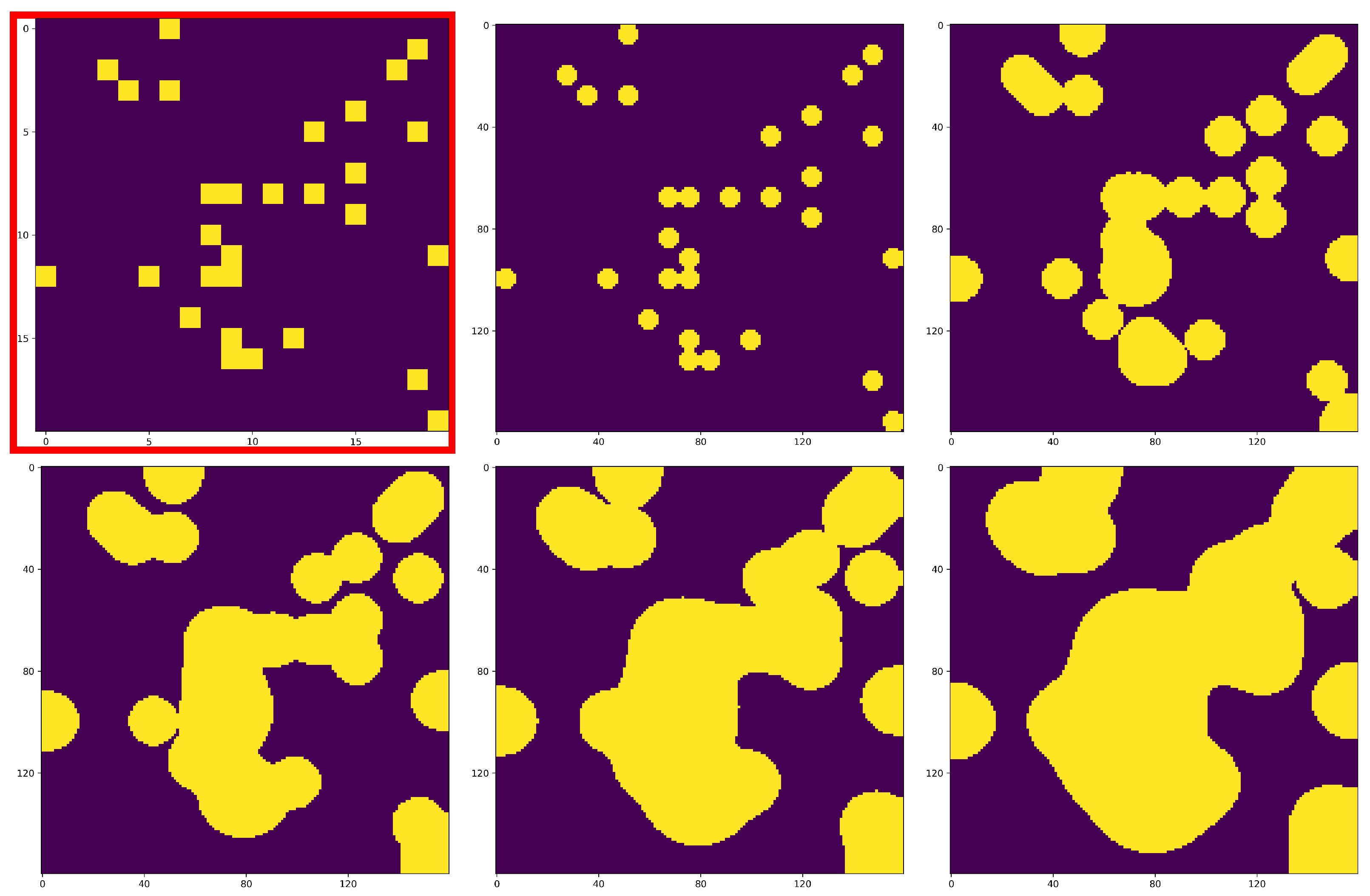
Some of the examples generated for a random droplet pattern image are shown in Figure 4.
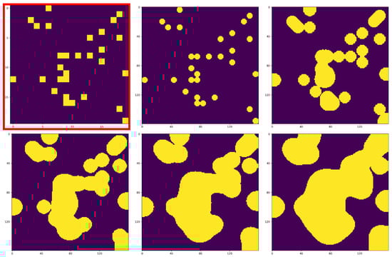
Figure 4.
Some of the examples from the dataset: a drop pattern image with pixels (red border) together with the evolution of the liquid film (imprint images with pixels) for various spread times: 0, 0.6 ms, 1.8 ms, 4.2 ms, and 8.0 ms, increasing from left to right and top to bottom. The corresponding liquid film thicknesses are 1 m, 263 nm, 179 nm, 140 nm, and 116 nm, decreasing from left to right and top to bottom.
We can see that the droplets spread and the film thickness reduces as time elapses. This phenomenon happens fairly quickly at the beginning, but it slows down over time.
2.2.2. Breakdown of the Compiled Dataset
We have run the physics-based solver to generate data for several categories based on the number of ‘On’ pixels in the droplet pattern image, i.e., the number of firing nozzles of the printhead to dispense droplet. More information about the breakdown of these datasets can be found in Table 1.

Table 1.
Breakdown of the compiled datasets.
The dataset for each category is provided independently from others. Some of the advantages include the following:
- Enabling researchers to select the categories that may best suit their application in the future.
- Providing a convenient way to properly prepare the training, validation, and test datasets from the data related to different categories not seen by each other.
- Reducing the size of the dataset by splitting it into smaller partitions.
When preparing the training, validation, and test datasets for a supervised learning task, one or multiple categories can be used partially or in its entirety. However, in order to mitigate the data leakage issue, one should be careful to not include examples with the same droplet pattern image in more than one dataset. This can be achieved by using data from different categories when preparing the training, validation, and test datasets. Alternatively, one can pre-process the data to ensure that the examples associated with the same droplet pattern image are not included in more than one of the training, validation, and test datasets.
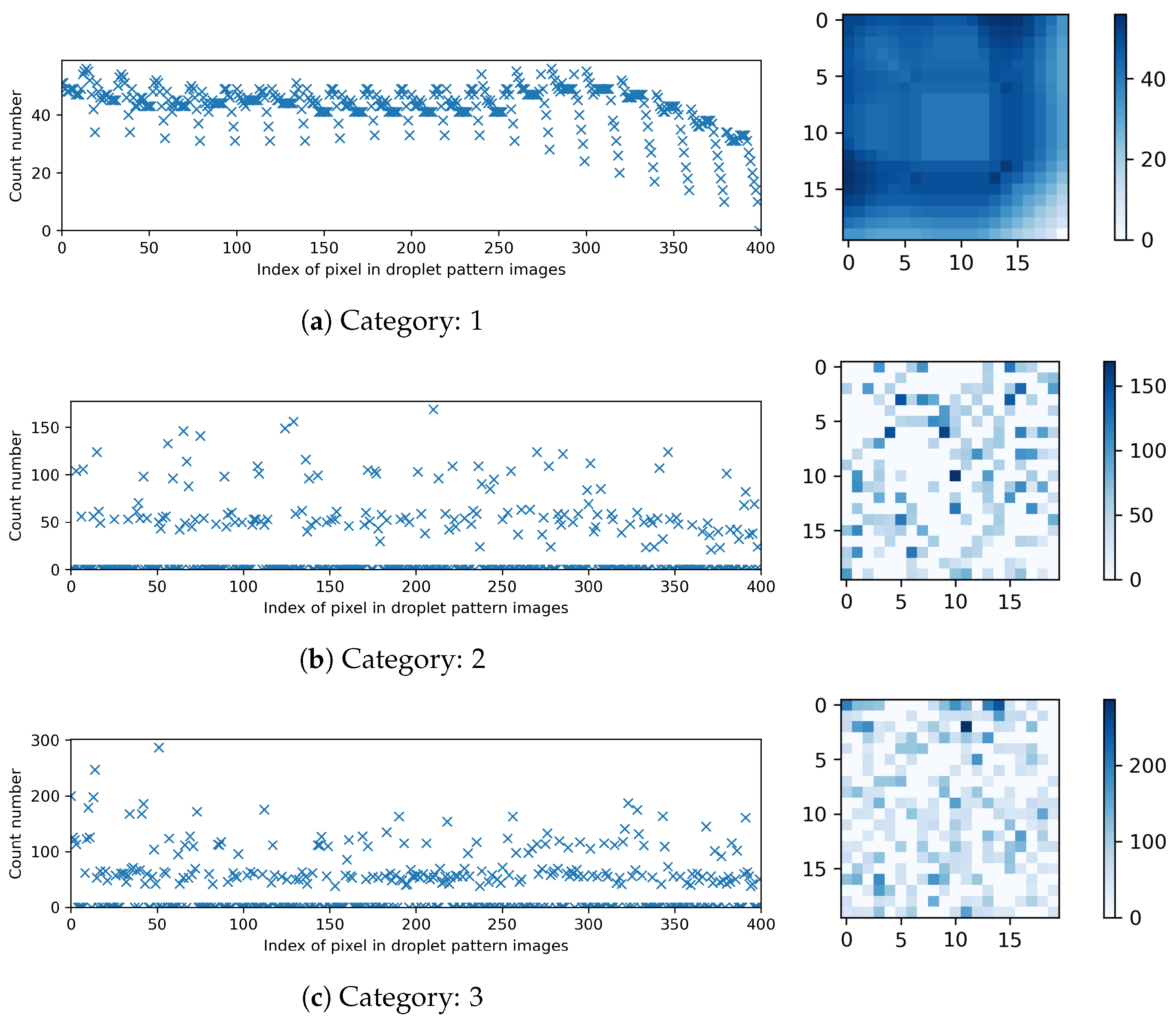
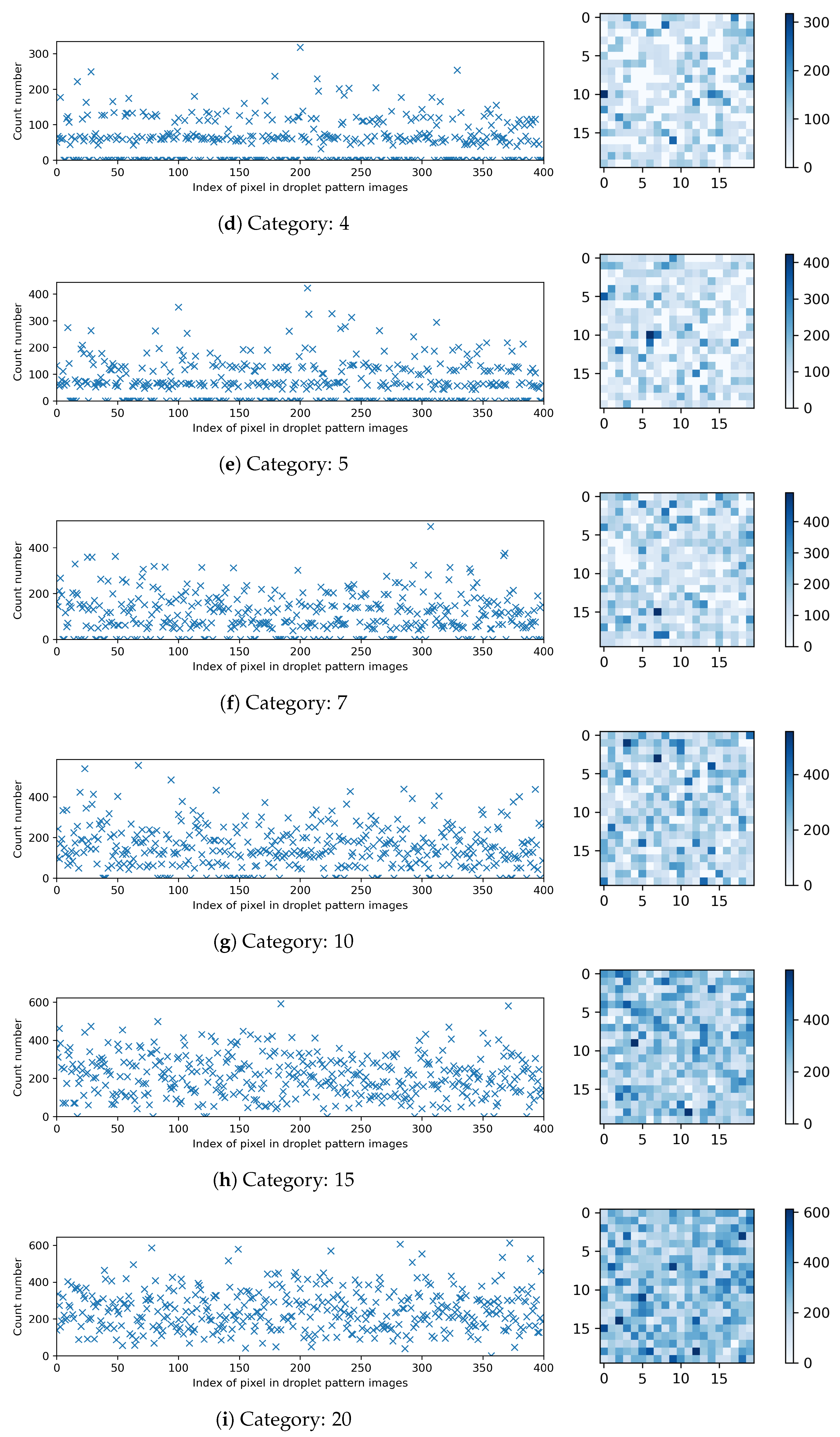
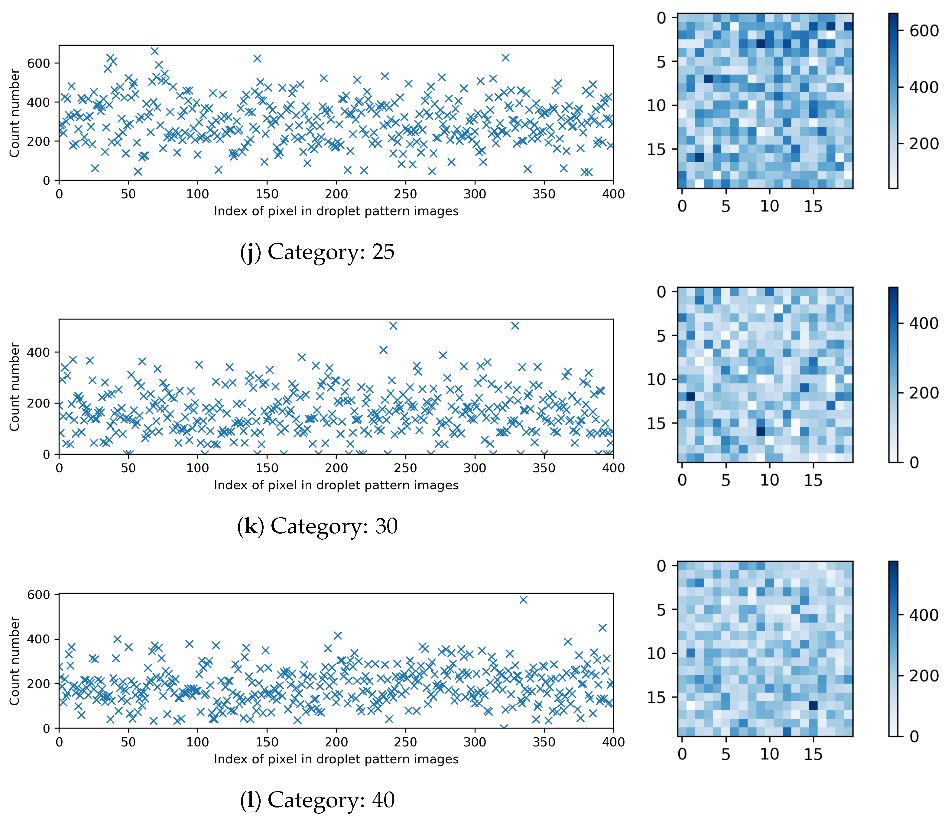
Figure 5 presents the breakdown of the compiled datasets for different categories in terms of the count number of occurrences for each pixel in the droplet pattern images.
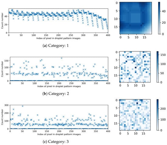
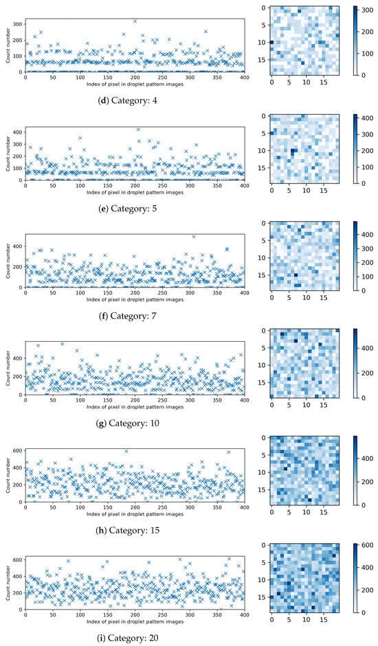
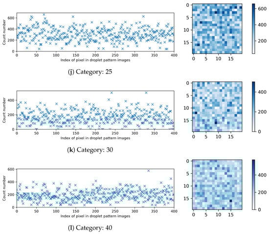
Figure 5.
Breakdown of the compiled datasets: the count number of occurrences for each pixel in the droplet pattern images with pixels.
2.2.3. Structure of Each Dataset
Each dataset includes four csv files:
- “t”–consisting of one column of data. The ith row holds the value of spread time (unit: second) for the ith example in that dataset partition.
- “h”–consisting of one column of data. The ith row holds the value of film thickness (unit: meter) for the ith example in that dataset partition.
- “dp”–consisting of multiple columns. The ith row holds the index of all ‘On’ pixels (value of 1) in the droplet pattern image for the ith example in that dataset partition. These pixels denote the firing nozzles of the printhead to dispense droplets. Other pixels are ‘Off’ (value of 0).
- “vof”–consisting of multiple columns. The ith row holds the index of all ‘On’ pixels (value of 1) in the imprint image for the ith example in that dataset partition. These pixels denote the wet area of the field. Other pixels are ‘Off’ (value of 0).
The developed Python package comes with some simple functions to read the dataset partition(s) from a given directory, or by walking through a root directory, and returning the compiled t, h, dp, and vof as NumPy arrays. The dp array has a shape of (dataset size, 400) since each drop pattern image has 400 pixels. The vof array has a shape of (dataset size, 25,600) since each imprint image has pixels.
2.3. A Gentle Dive into the Fluid Dynamics of the System
Before using the dataset, it is good to have some level of familiarity with the underlying physics of the system that the dataset is derived from. For example, an accurate and robust image-to-image mapping is not achievable by solely considering the dp and vof images in their entirety. Any reasonable mapping between these images in their entirety should capture the strongly non-linear correlation of these images with each other and also with the spread time and liquid film thickness. Alternatively, one may omit the effects of spread time (or liquid film thickness) by confining the dataset to a narrow range of spread time (or liquid film thickness).
In this section, we aim at explaining, from a high-level perspective, how the parameters of an example are correlated qualitatively: t (scalar), h (scalar), dp (drop pattern image), and vof (imprint image).
Let us start with a simple system with only one droplet (Example 1) as shown in Figure 6 (top). As we can see, only one pixel of the dp is ‘On’. At the beginning of the imprinting process, the imprint image reasonably resembles the drop pattern image, except that it has pixels compared to pixels of the drop pattern image. As time elapses, the droplet spreads further and the liquid film thickness decreases (conservation of mass principle); please see Figure 7.
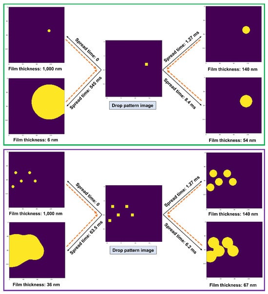
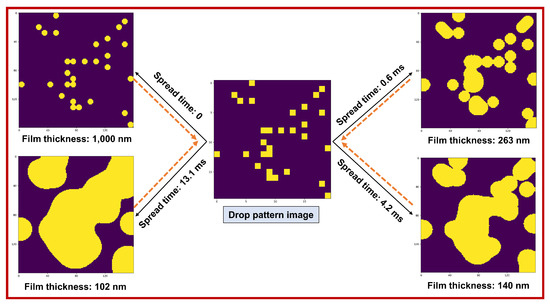
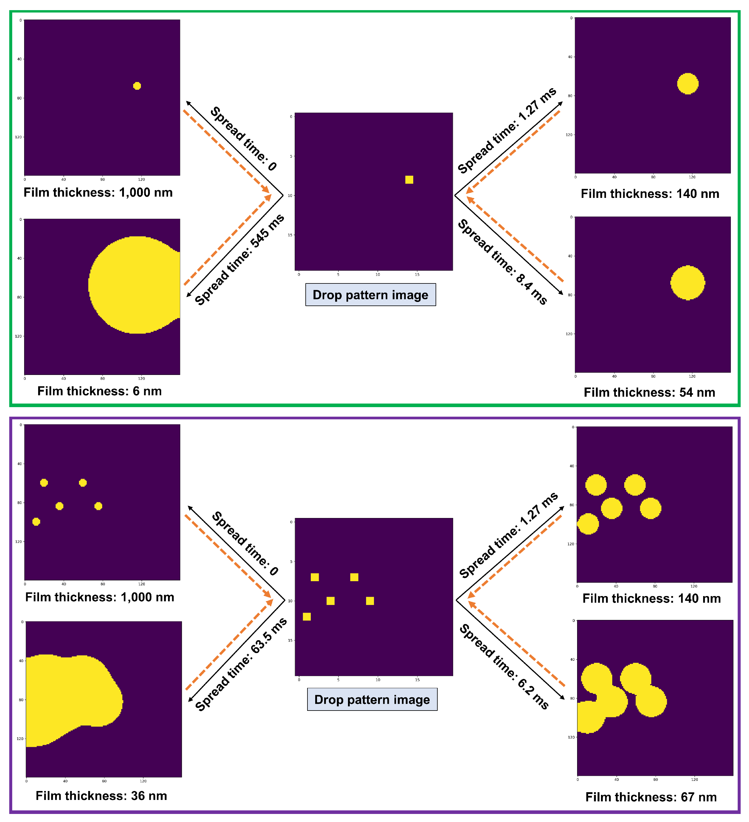
Figure 6.
The liquid film map (imprint image vof) for different spread times given three different drop pattern images (dp): Example 1 (top), Example 2 (middle), and Example 3 (bottom). The solid black arrows show the translation of the drop pattern image to an imprint image for different spread times (forward problem). The orange dashed arrows denote the translation of an imprint image with a given film thickness to an appropriate drop pattern image and the required spread time (inverse problem). Here, the droplet pattern images have pixels, while the imprint images contain pixels.
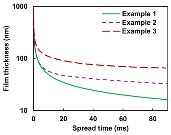
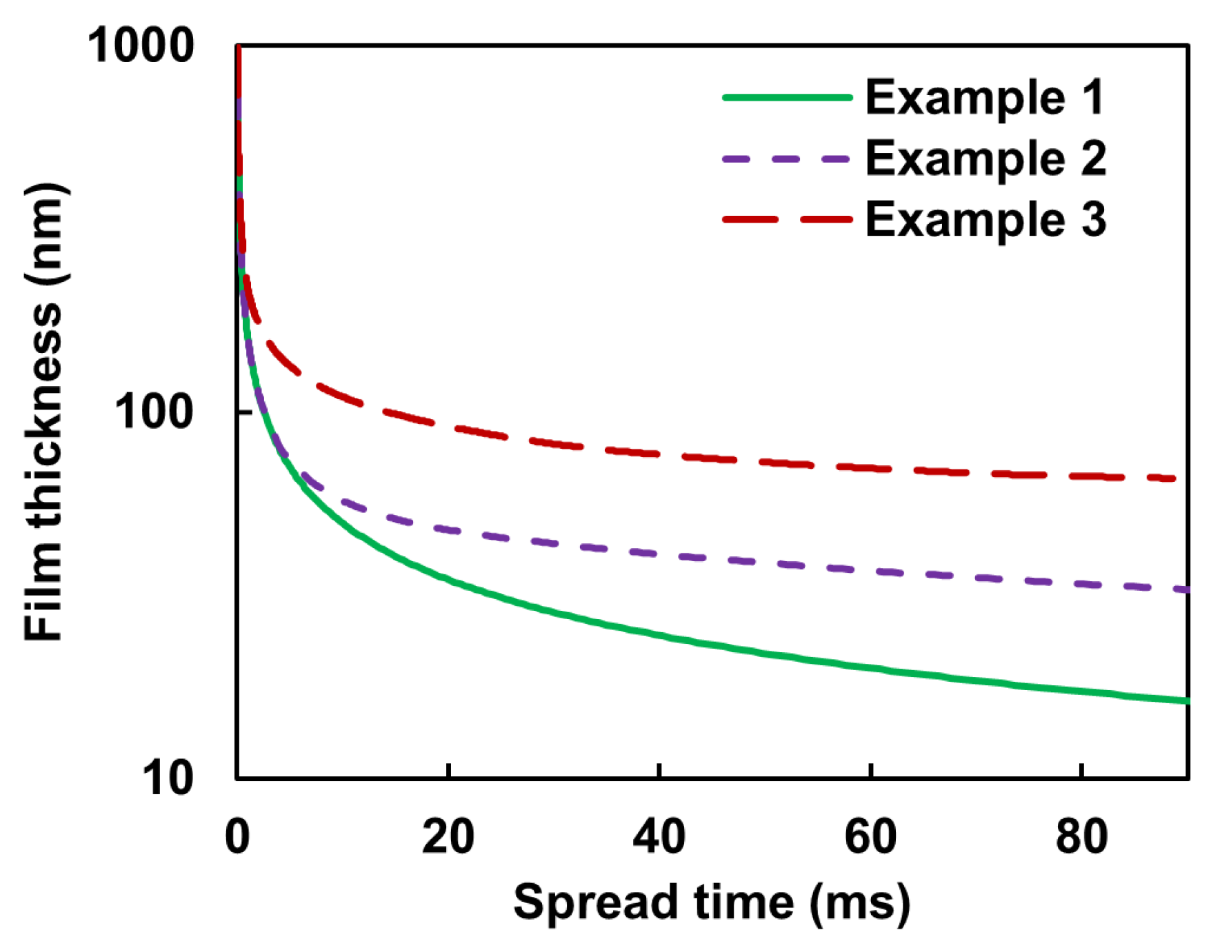
Figure 7.
The temporal evolution of the film thickness for three different drop pattern images presented in Figure 6.
The dynamics of the system is relatively fast at the beginning, but it becomes slower with time (attenuation of both film thinning rate and droplet spreading velocity). For example, it takes about 1.27 ms for the liquid film thickness to reduce from 1 m to 140 nm, while it needs another 7.13 ms, i.e., a total spread time of 8.4 ms, to get to 54 nm film thickness.
Now, let us consider a dp image with only five ‘On’ pixels (Example 2) as shown in Figure 6 (middle). The dynamics of the system is the same as the previous one until the droplets start to merge, i.e., it takes about 1.27 ms for the liquid film thickness to reduce from 1 m to 140 nm. However, the current system becomes slower than the previous one as a result of the merging of droplets. This behavior can be discerned more easily from Figure 7, which shows the dynamic evolution of the liquid film thickness.
Similarly, the same fluid flow characteristics can be observed for a dp image with 29 ‘On’ pixels (Example 3) as shown in Figure 6 (bottom), except that the merging of droplets that are, now, more in quantity and closer to each other in some areas, causes the dynamics of the system to become slower than in Example 2. Figure 7 should help to more easily observe this behavior. The key takeaway from Figure 6 and Figure 7 is that the system’s dynamics slow down over time following more droplet merging.
2.4. Network Structure
The basic principle of our proposed model is to train and tune the refinement level of convolutional layers. At the core of this convolutional neural network with a trainable and tunable refinement level (CNN-TTR) is residual convolutional blocks with tunable refinement (CNN-TR) connected to function approximators that are trained to find the optimal refinement level. The refinement level of CNN-TR blocks is then tuned by the trained function approximator. A schematic representation of our proposed CNN-TTR model is depicted in Figure 8.
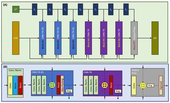
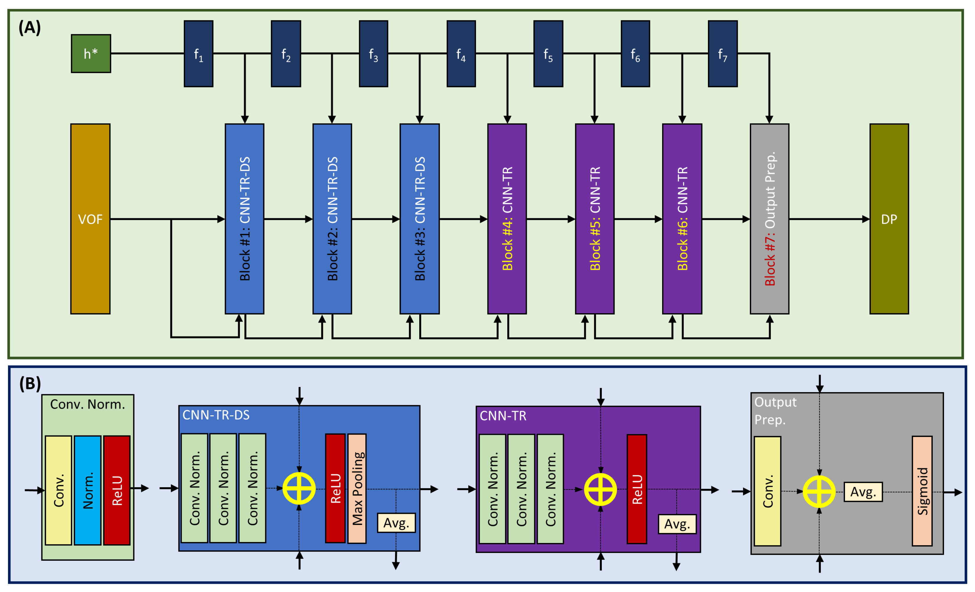
Figure 8.
(A) The architecture of our residual convolutional neural network with a trainable and tunable refinement level (CNN-TTR) to map a high-resolution imprint image (VOF), in conjunction with a normalized film liquid thickness , to its target low-resolution droplet pattern image (DP), as well as (B) the building blocks used in our model.
Our convolutional neural network consists of components to accomplish the following tasks:
- Function approximation: dense blocks of aiming at predicting the appropriate refinement level in each stage.
- Down-scaling: a stack of convolutional layers with tunable refinement and down-scaling (CNN-TR-DS). An input image with pixels is down-scaled to (Block #1), (Block #2), and pixels (Block #3) sequentially.
- Widening of field of view: a stack of convolutional layers with tunable refinement and no down-scaling (CNN-TR).
- Output preparation: a convolutional layer with tunable refinement and a sigmoid activation function.
2.4.1. Function Approximation
The similarity between an imprint image vof and its target drop pattern image dp decreases as the droplets spread and merge further with time. As a result, in order to predict the target dp image, more refinement (removing ‘On’ pixels properly) of the vof image is required. Finding the appropriate refinement level in each stage is accomplished by a function approximator. Such function approximators aim at finding the appropriate refinement levels to be used by their corresponding residual convolutional blocks with tunable refinement (CNN-TR and CNN-TR-DS). Here, a function approximator [41] is a dense neural network with one hidden layer of 128 units and an activation function of ReLU [42].
2.4.2. Convolutional Blocks with Tunable Refinement with (CNN-TR-DS) and Without (CNN-TR) Down-Scaling
Each CNN-TR and CNN-TR-DS block has three inputs: 1. feature maps from the preceding block, 2. a single map consisting of the element-wise average of the feature maps from the preceding block, and 3. a refinement level indicator provided by the corresponding function approximator. Providing the average of the feature maps of the last preceding block enables access to the corresponding hierarchical features and mitigate the loss of information that should be preserved.
Each CNN-TR and CNN-TR-DS block consists of a stack of three connected Conv. Norm. blocks. The output of this stack is added (element-wise) to inputs #2 and 3: the refinement level indicator and the average feature map from the last preceding block. The difference in CNN-TR and CNN-TR-DS is that the latter uses a max pooling layer for down-scaling while CNN-TR blocks are used to widen the field of view.
Each Conv. Norm. block comprises a convolutional layer with the kernel size of 5, followed by an instance normalization [43] and ReLU activation function [42]. For the CNN-TR-DS blocks, each convolutional layer has 32, 64, and 128 filters in Blocks #1, 2, and 3, respectively. For the CNN-TR blocks, each convolutional layer has 128, 64, and 32 filters in Blocks #4, 5, and 6, respectively.
2.4.3. Output Preparation Block
Block #7 is similar to a CNN-TR block with the difference being that it has only one convolutional layer with no normalization or ReLU activation. It has a sigmoid activation function at the end of the block. The convolutional layer in this block has 8 filters with a kernel size of 5.
3. Results and Discussion
3.1. Pre-Processing
When preparing the training, validation, and test datasets, we selected data from different categories according to Table 2.
Table 2.
Fraction of each category selected for pre-processing when preparing training, validation, and test datasets.
To ensure that the network properly learns both droplet spreading and merging dynamics, our training dataset was designed to include the following:
- Pure spreading dynamics: Isolated single droplets and widely spaced multi-droplet cases;
- Merging dynamics: Interacting droplets with varying degrees of liquid film interaction.
This approach enables comprehensive exposure to the underlying physics, from individual droplet behavior to complex coalescence phenomena.
To mitigate the issue with examples that can potentially have multiple solutions, we omitted the examples with too large continuous liquid film in their vof image. We displaced an interrogation window with pixels across each vof image. Any example with a local coverage greater than was removed from the datasets. The final number of examples in the training, validation, and test datasets is shown in Table 3.
Table 3.
Number of examples in training, validation, and test datasets after pre-processing.
We use and as the normalized scalars for t and h, respectively, as defined below:
wherein and refer to the arithmetic mean and standard deviation of for the examples within the training dataset, respectively. Similarly, and refer to the arithmetic mean and standard deviation of for the examples within the training dataset, respectively. The distribution of and is shown in Figure 9 for the training, validation, and test datasets.
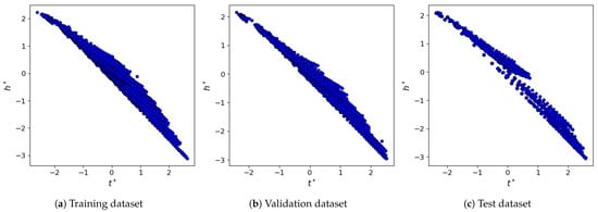
Figure 9.
The distribution of and for the training, validation, and test datasets.
3.2. Training
The model has 3,085,935 trainable parameters in total. We used TensorFlow [44] and Keras [45] to train our model. The model was trained using Adam optimization [46], with binary cross entropy loss, while regularization was applied to the bias and kernel of the convolutional layers to prevent overfitting.
We use the precision–recall (PR) plot and the associated area under curve (AUC) metric to evaluate the performance of our model. On average, only about of pixels of dp images are ‘On’, which leads to an imbalanced dataset. We noticed that in our case, because of having an imbalanced dataset, the AUC of receiver operating characteristics (ROCs) misleadingly leads to a much higher value than the AUC-PR. Therefore, the AUC-ROC could be deceptive when drawing conclusions about the performance of the model on the current dataset wherein the number of negatives outweighs the number of positives significantly. This observation is in agreement with the existing literature. For example, interested readers can find more detailed discussion on imbalanced datasets and how they affect PR and ROC from Saito and Rehmsmeier [47].
The validation dataset was used to examine the performance of the trained model for various classification thresholds. The results are shown in Figure 10a in terms of precision, recall, and F-1 score.
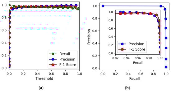
Figure 10.
(a) The variations in precision, recall, and F-1 score with the classification threshold when running the model on the validation dataset. (b) The precision–recall plot as well as (inset) the F-1 score variations for the magnified region of interest.
The PR curve is also presented in Figure 10b. The obtained AUC-PR for the validation dataset equals . The PR curve shows an acceptable performance over a wide range of thresholds, but the highest F-1 score related to the validation dataset is found when the threshold is about . The corresponding F-1 score is . Finally, by using this optimized model and classification threshold, we obtain the F-1 score of on the test dataset.
We used the test dataset to compare the trained model’s performance with that of a crude model consisting of three max pooling layers with no trainable parameters. The results are shown in Table 4.
Table 4.
Comparison of the performances of the model CNN-TTR and a crude model consisting of three max pooling layers without any trainable parameter when acting on the test dataset. Here, the threshold equals 0.5 when calculating the precision, recall, and F-1 score.
As expected, the crude model can predict all the ‘On’ pixels of the dp images (Recall = 1.0) at the cost of a relatively low precision of about 11.59%.
3.3. Function Approximators
The output of neural network function approximators is shown in Figure 11 for various values.
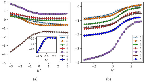
Figure 11.
(a) The output of function approximators for various values using the trained model CNN-TTR and (b) its counterpart with a linear activation function within the CNN-TR and CNN-TR-DS blocks and no normalization layer in the Conv. Norm. blocks.
Figure 11a shows the results for the trained model CNN-TTR, the schematic representation of which is shown in Figure 8. When drawing conclusions about these results, we need to keep in mind that the model CNN-TTR consists of an instance normalization layer within the Conv. Norm. blocks and the nonlinear activation function of ReLU within the CNN-TR and CNN-TR-DS blocks, as a result of which the observed trends my not be easily interpretable. Nevertheless, the plot shows that, in general, the outputs are negative. Together with the immediate ReLU activation function within the CNN-TR and CNN-TR-DS blocks, such negative translations lead to a sequential refinement, i.e, a removal of ‘On’ pixels of image in a sequential fashion.
Figure 11b shows the results for a less effective (slower training and lower AUC-PR) variant of CNN-TTR with a linear activation function within the CNN-TR and CNN-TR-DS blocks and no normalization layer within the Conv. Norm. blocks. Because of omitting the non-linearity associated with the aforementioned components, the behavior of function approximators is, now, more interpretable: a vof image with a thinner liquid film (smaller ) requires more refinement to obtain its target dp image. Hence, the function approximators output a smaller value (a negative number with a larger magnitude) as decreases, leading to a larger refinement level (the removal of more ‘On’ pixels).
3.4. Sequential Refinement
The concept of sequential refinement is demonstrated in Figure 12 for a given example from the test dataset.
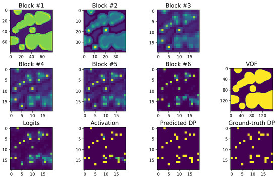
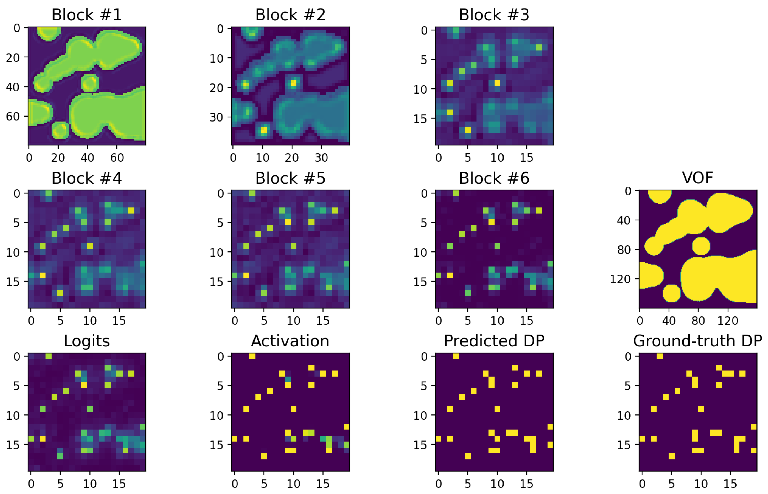
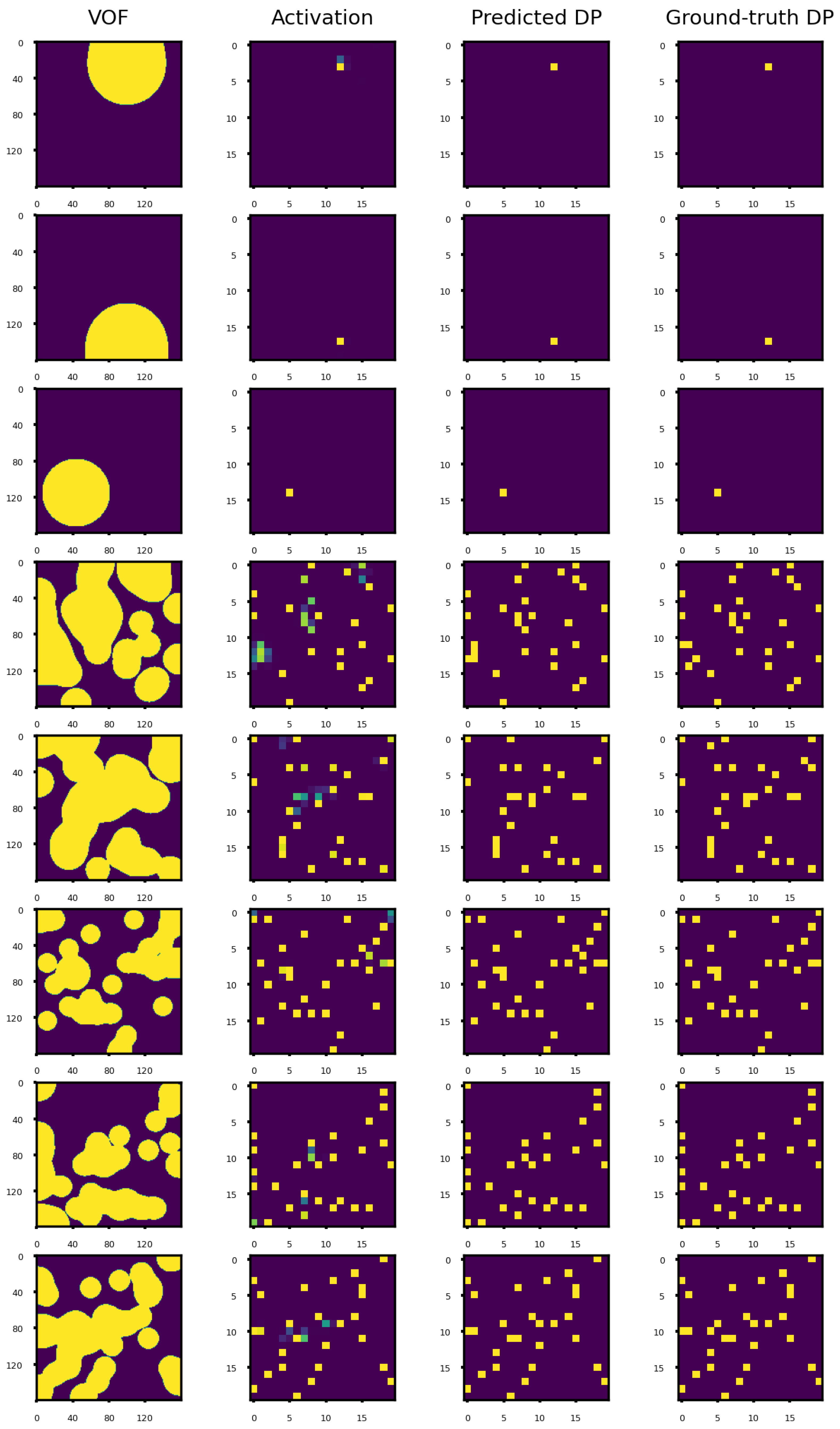
Figure 12.
The average response maps of Blocks #1–6 as well as the logits and the sigmoid activation map related to Block # 7, together with the ground-truth dp image for a given example from the test dataset with .
The model refines the vof image in multiple steps based on the normalized thickness of the liquid film until the predicted dp image is obtained. It can be discerned that a region with a relatively small puddle of liquid is more easily refined while an area with a large continuous liquid film is more challenging to refine properly.
There are two potential culprits for the problem associated with the large-coverage regions: 1. insufficient examples during the training of model, and 2. the non-uniqueness of the solution for such regions. In particular, a large-coverage region may be obtainable by multiple droplet patterns that differ only slightly in one or a few pixels (usually close to the center of such large-coverage regions).
One of the consequences of the model getting less confident in these situations is that some of the ‘On’ pixels can be lost when using the classification threshold optimized for the highest F-1 score. In such situations, reducing the classification threshold can lead to a higher recall value at the cost of reducing the precision and F-1 score. However, as shown in Figure 10, the model performs acceptably well on a wide range of the classification threshold. Hence, one can reduce the classification threshold to improve the recall metric. We have noticed that the subsequent reduction in precision is partly due to the slight misplacement of one or few ‘On’ pixels close to the center of large-coverage regions, which is still much better than completely losing those ‘On’ pixels. The results obtained using a classification threshold of 0.4 are shown in Figure 13 for some of the examples from the test dataset.
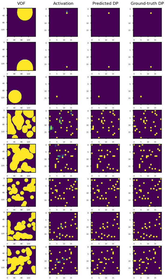
Figure 13.
Prediction of the model CNN-TTR for several examples from the test dataset. Here, the classification threshold equals 0.4 when obtaining the “Predicted DP” from the sigmoid layer’s activation. From top to bottom, is −2.641, −2.574, −2.435, −0.173, −0.136, 0.317, 0.169, and 0.123.
3.5. Kernels
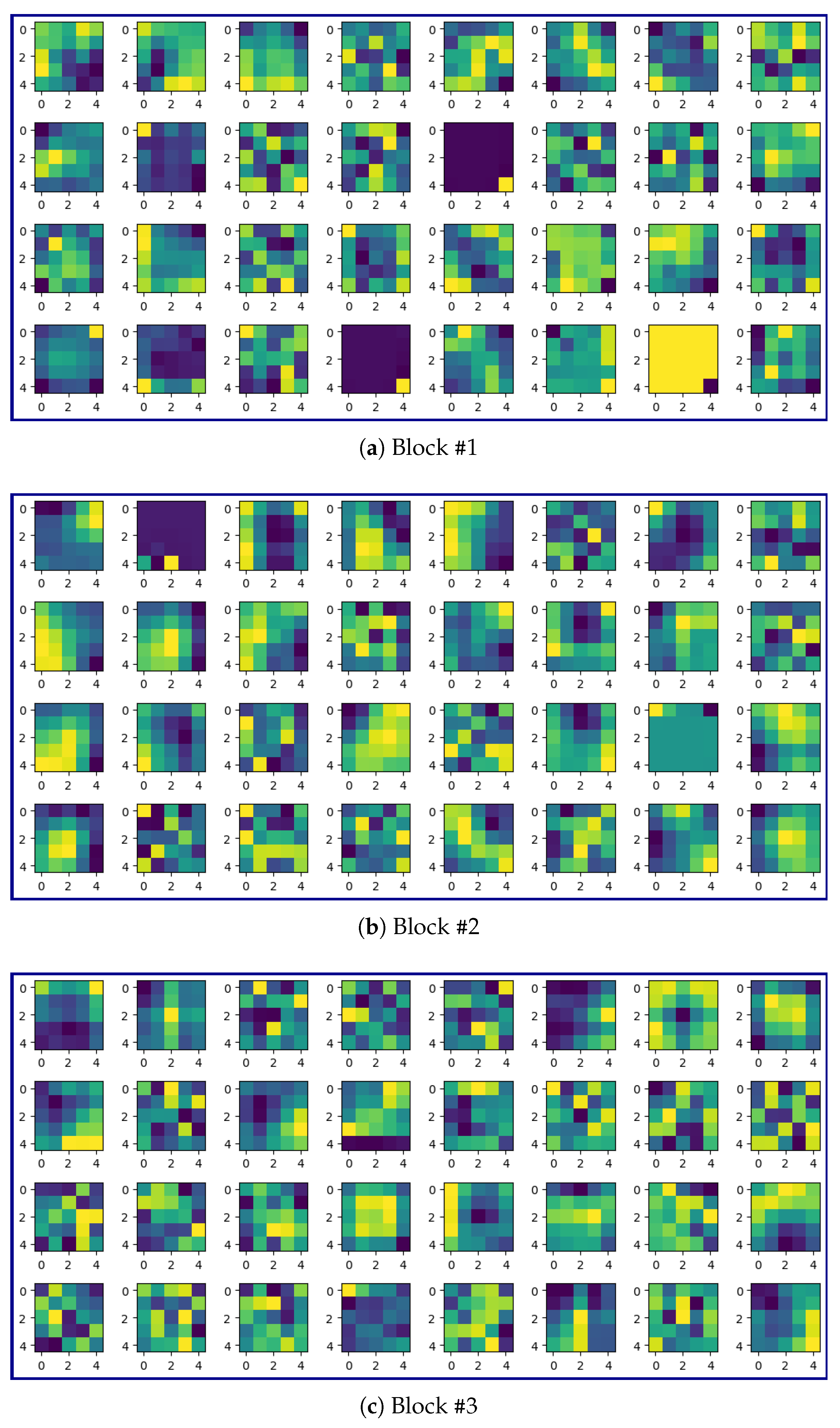
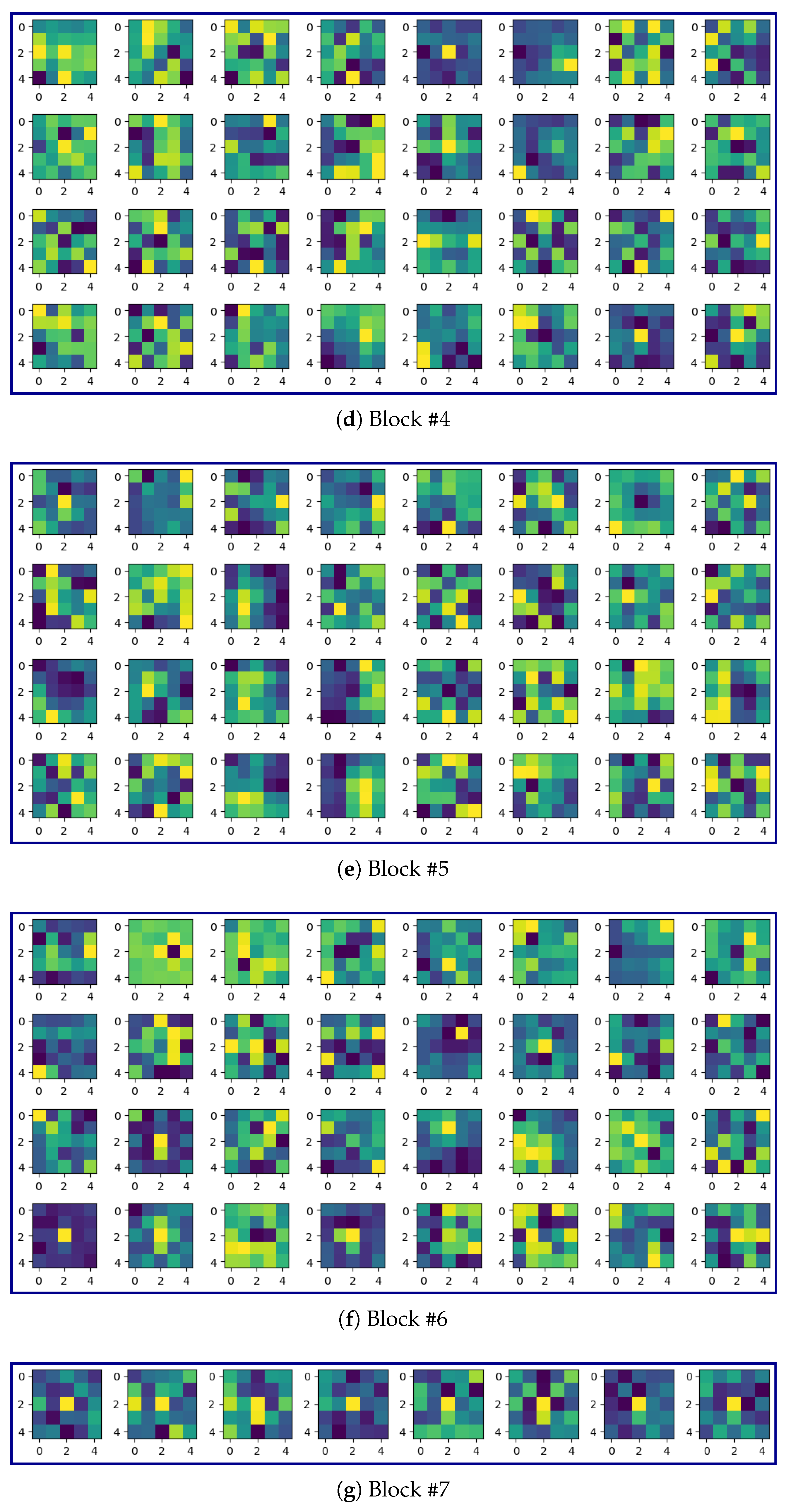
Some of the kernels of the first convolutional layer in Blocks #1–7 are shown in Figure 14.
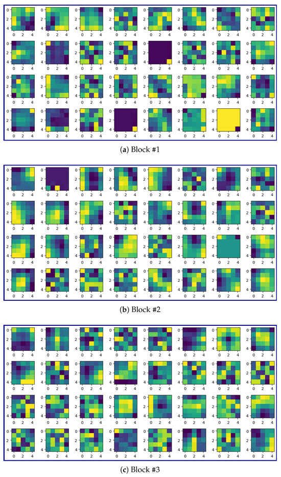
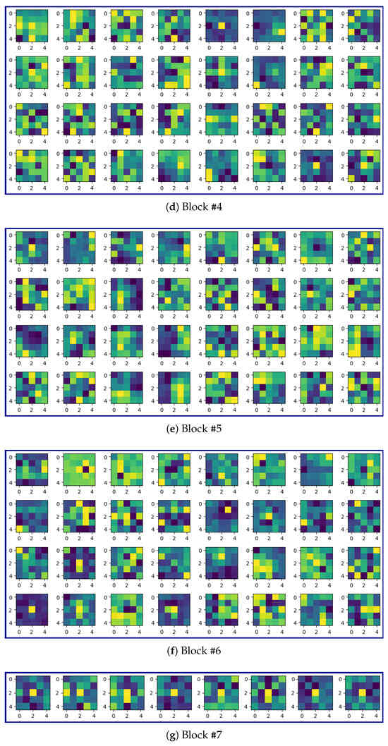
Figure 14.
Some of the kernels of the first convolutional layer for different Blocks (normalized to vary between 0 and 1).
Figure 14 demonstrates the progressive specialization of convolutional kernels across network depth. In early blocks, e.g., Block #2, kernels predominantly exhibit edge-detection configurations (for example, Figure 14b, column 1) that optimally capture liquid–gas interfaces. In contrast, deeper blocks (e.g., Block #7) develop more complex activation patterns (a central pixel with surrounding activations) that effectively detect local droplet arrangements. This hierarchical feature learning mirrors the physical scales present in our problem, from micron-scale interface curvature to millimeter-scale droplet patterns.
3.6. Custom Image
In order to examine how the model performs on a custom image, we used an image of the letter ‘A’ as shown in Figure 15 (left).
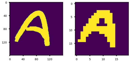
Figure 15.
(Left) A custom image of the letter ‘A’ together with (Right) the droplet pattern produced by a crude model consisting of three max pooling layers with no trainable parameters.
A crude model consisting of three max pooling layers with no trainable parameters predicts a droplet pattern with 97 ‘On’ pixels (number of droplets to be dispensed) as shown in Figure 15 (right).
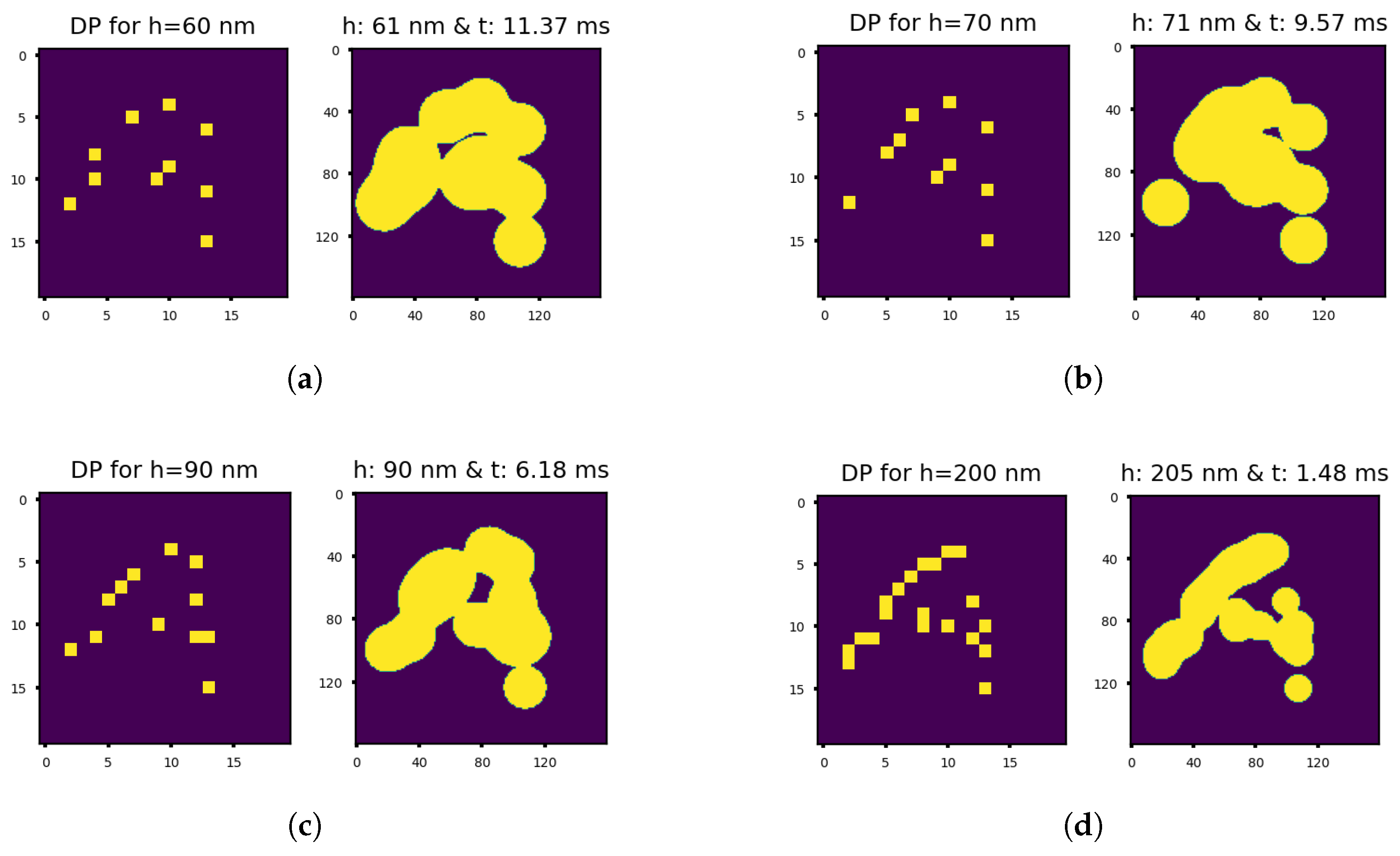
We used the CNN-TTR model to predict the droplet pattern images for different target liquid film thicknesses (classification threshold of 0.3). Some of the results are shown in Figure 16.
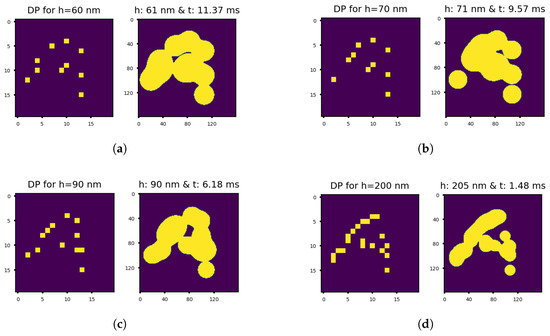
Figure 16.
(Left) The droplet pattern image (DP) predicted by the CNN-TTR model for the custom image of the letter ‘A’ shown in Figure 15 together with the (Right) corresponding imprint image obtained from the physics-based solver using the predicted droplet pattern image for different cases wherein the target liquid film thickness equals (a) 60 nm, i.e., , (b) 70 nm, i.e., , (c) 90 nm, i.e., , and (d) 200 nm, i.e., .
It can be perceived that the model generally predicts a lower number of droplets (‘On’ pixels in the dp image) to be dispensed for thinner liquid films (10–20 droplets) since the droplets spread more while the liquid film thickness reduces to a smaller value.
In the next step, we examined the droplet patterns predicted for these inverse problems, i.e., left images in Figure 16a–d. We used the physics-based solver to find the imprint vof image for the predicted droplet pattern and the corresponding target liquid film thickness: right images in Figure 16a–d.
We notice that the obtainable imprint images do not have as high a resolution as the input image of the letter ‘A’ shown in Figure 15. This can be attributed to the finite size of droplets (6 pl in this work) and the fact that they become even larger (lower obtainable resolution) as the liquid film is squeezed further. As a result, the best obtainable resolution is dictated by the size of droplets dispensed by the printhead.
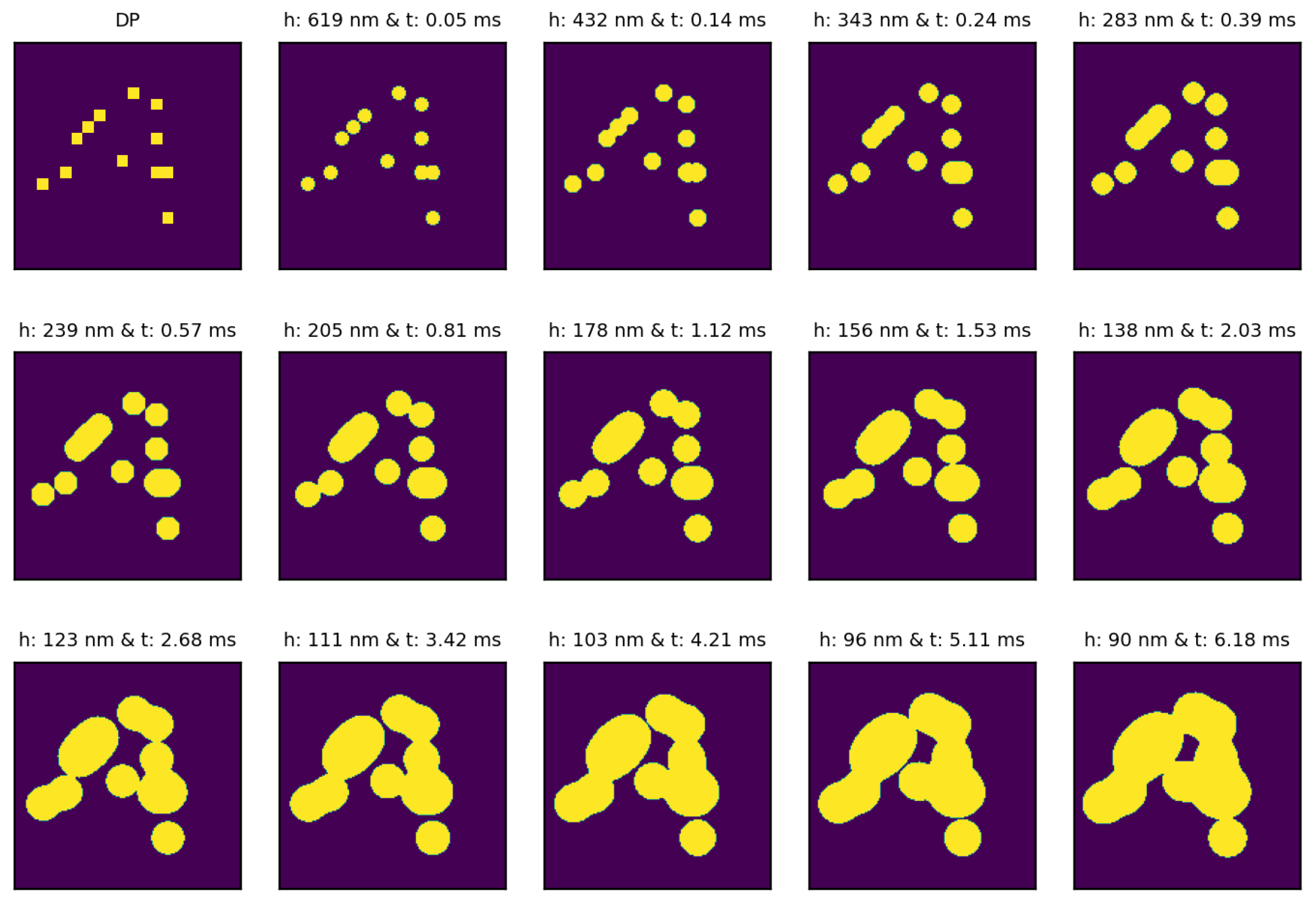
The time series imprint vof images obtained by using the physics-based solver for the case of the target liquid film thickness of 90 nm are shown in Figure 17.
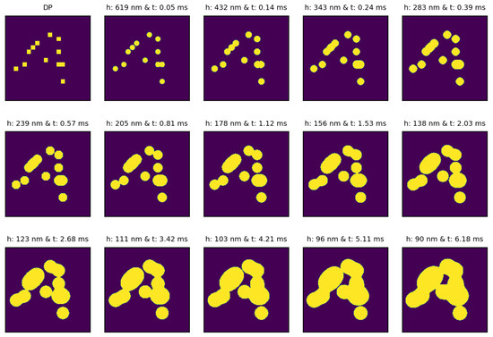
Figure 17.
The droplet pattern produced by the CNN-TTR model for a custom image of the letter ‘A’ shown in Figure 15 and the target liquid film thickness of 90 nm, i.e., , together with the time series imprint vof images obtained from the physics-based solver for the predicted droplet pattern image.
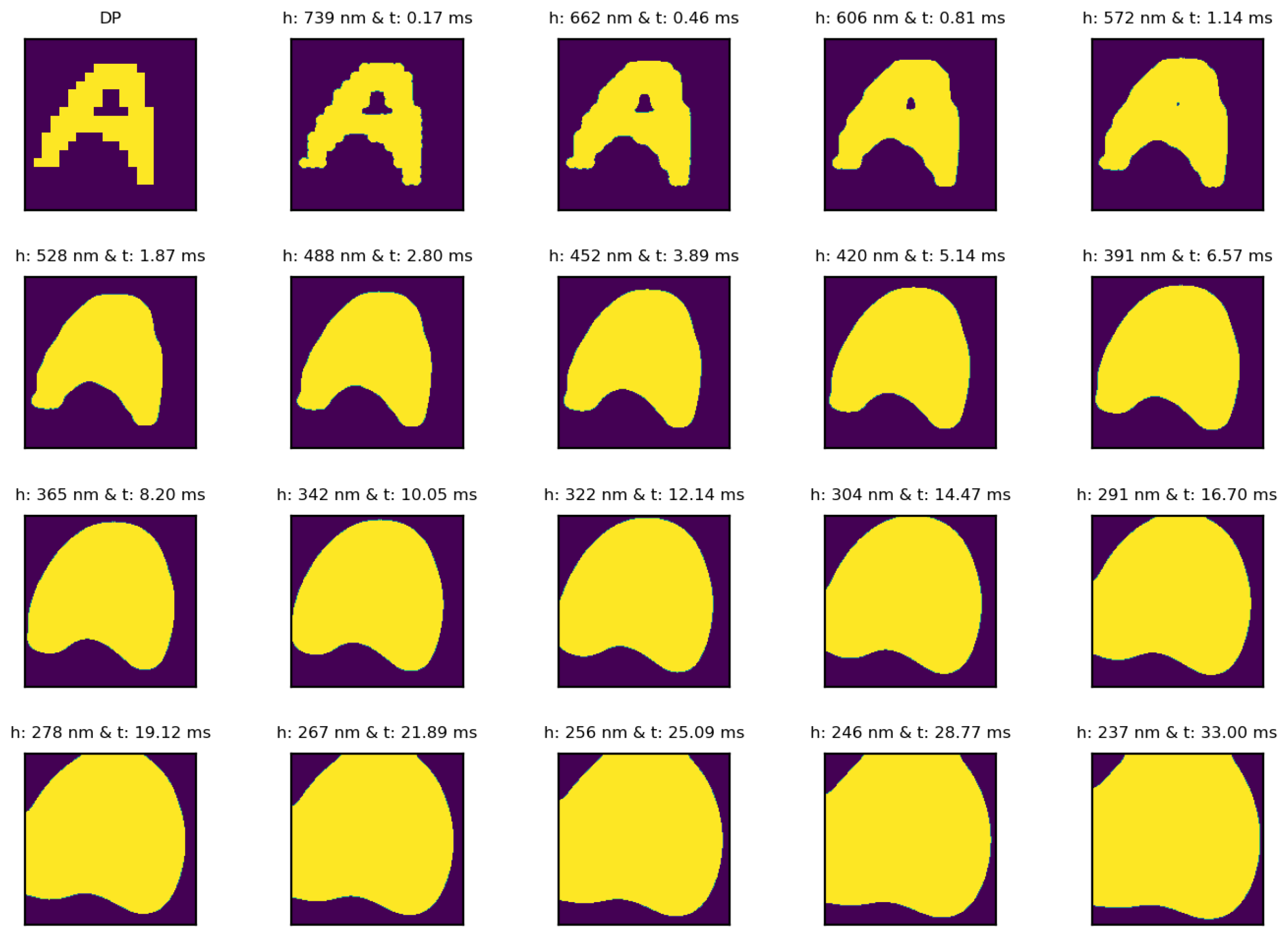
The corresponding results related to the droplet pattern predicted by a crude model consisting of three max pooling layers with no trainable parameters are also shown in Figure 18.
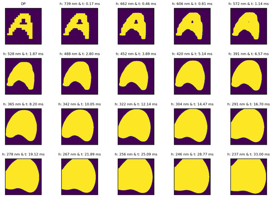
Figure 18.
The droplet pattern produced by a crude model consisting of three max pooling layers with no trainable parameters for a custom image of the letter ‘A’ shown in Figure 15 together with the time series imprint vof images obtained from the physics-based solver for the predicted droplet pattern image.
We can see that the crude model’s performance deteriorates as the liquid film thickness decreases since it does not take into account the spreading and merging of droplets.
4. Future Works
While we have not performed a systematic study investigating the droplet volume effects on minimum resolvable feature size, we expect that smaller droplets improve resolution. The precise quantification of this relation, however, warrants future investigation.
Moreover, the present study focuses on a specific range of liquid film thicknesses under fixed viscosity and surface tension conditions based on requirements for our internal process developments. While this enables a controlled examination of key parameters, e.g., capillary force and interfacial dynamics, as well as the spreading and merging of droplets, it inherently limits the application of the trained model to other applications. Variations in viscosity and surface tension are known to significantly influence thin-film behavior: increased viscosity typically reduces the droplets spread speed while reduced surface tension can diminish the capillary driving force, reducing the spread speed. Future studies could explicitly vary fluid properties to map their influence on characteristic behaviors.
In addition, the results of the inverse problems shown in Figure 16 can be improved by human/physics-based solver intervention, i.e., using the model’s predicted droplet pattern image as a starting point to add, remove, or displace droplets for a more desired outcome. Hence, future efforts can be devoted to two purposes: 1. improving the neural network model and 2. enhancing the neural network model by including the physics-based solver in the decision making process. Therefore, some of the potential future works could include:
- Including both the neural network (inverse problem) and physics-based solver (forward problem) in the decision making process.
- Extending the dataset to include smaller droplets that can potentially lead to higher-resolution patterns.
- Extending the dataset to include various droplet diameters to increase the flexibility of generating droplet patterns for higher-resolution patterns.
5. Conclusions
In this paper, we proposed a residual convolutional neural network with a new structure suitable for refining a high-resolution image to a low-resolution one. We demonstrated the concept in the context of squeeze flow of micro-droplets. We showed that the CNN-TTR model learns to systematically tune the refinement level of its residual convolutional blocks by using multiple function approximators. We believe that this work can find value in the semiconductor manufacturing and packaging industry. In the future, the dataset can be extended to include various droplet volumes to enhance the flexibility of generating droplet pattern maps for producing higher-resolution imprint patterns. The proposed framework could also be applied to data compression and encryption. It may enable lightweight low-resolution data communication, where the corresponding high-resolution format can be reconstructed using the forward model on either end of the transmission. Additionally, the developed package and compiled datasets could serve as free, flexible, and scalable standardized benchmarks for tasks such as time series image analysis, multi-class, multi-label classification (with numerous classes/labels), image deblurring, and related applications.
Author Contributions
Conceptualization, A.M.; methodology, A.M.; software, A.M.; validation, A.M.; formal analysis, A.M.; investigation, A.M.; resources, A.M., S.S. and S.V.S.; data curation, A.M.; writing—original draft preparation, A.M.; writing—review and editing, A.M., S.S. and S.V.S.; visualization, A.M.; supervision, S.S. and S.V.S.; project administration, A.M. and S.S.; funding acquisition, S.V.S. All authors have read and agreed to the published version of the manuscript.
Funding
This research received no external funding.
Data Availability Statement
The developed package and datasets are publicly available on GitHub at https://github.com/sqflow/sqflow (accessed on 20 July 2025).
Acknowledgments
The authors acknowledge the Texas Advanced Computing Center (TACC) at The University of Texas at Austin for providing HPC resources that have contributed to the research results reported within this paper. URL: http://www.tacc.utexas.edu.
Conflicts of Interest
The authors declare no conflicts of interest.
References
- Kalliadasis, S.; Bielarz, C.; Homsy, G.M. Steady free-surface thin film flows over topography. Phys. Fluids 2000, 12, 1889–1898. [Google Scholar] [CrossRef]
- Balestra, G.; Badaoui, M.; Ducimetière, Y.-M.; Gallaire, F. Fingering instability on curved substrates: Optimal initial film and substrate perturbations. J. Fluid Mech. 2019, 868, 726–761. [Google Scholar] [CrossRef]
- Pettas, D.; Karapetsas, G.; Dimakopoulos, Y.; Tsamopoulos, J. Stability analysis of a Newtonian film flow over hydrophobic microtextured substrates. Phys. Rev. Fluids 2022, 7, 034004. [Google Scholar] [CrossRef]
- Pettas, D.; Dimakopoulos, Y.; Tsamopoulos, J. Steady flow of a viscoelastic film over an inclined plane featuring periodic slits. J. Non-Newton. Fluid Mech. 2020, 278, 104243. [Google Scholar] [CrossRef]
- Engmann, J.; Servais, C.; Burbidge, A.S. Squeeze flow theory and applications to rheometry: A review. J. Non-Newton. Fluid Mech. 2005, 132, 1–27. [Google Scholar] [CrossRef]
- Liu, C.; Guo, F.; Li, X.; Li, S.; Han, S.; Wan, Y. Experimental study of elastohydrodynamic lubrication behaviour under single oil droplet supply. Tribol. Int. 2018, 118, 432–440. [Google Scholar] [CrossRef]
- Lang, J.; Santhanam, S.; Wu, Q. Exact and approximate solutions for transient squeezing flow. Phys. Fluids 2017, 29, 103606. [Google Scholar] [CrossRef]
- Aghkand, Z.K.; Ajji, A. Squeeze flow in multilayer polymeric films: Effect of material characteristics and process conditions. J. Appl. Polym. Sci. 2022, 139, 51852. [Google Scholar] [CrossRef]
- Barakat, J.M.; Hinton, Z.; Alvarez, N.J.; Walker, T.W. Surface-tension effects in oscillatory squeeze flow rheometry. Phys. Fluids 2021, 33, 122112. [Google Scholar] [CrossRef]
- Ha, K. Axisymmetric squeezing dynamics of resin droplet with surface tension and its numerical solution. J. Mech. Sci. Technol. 2019, 33, 5861–5880. [Google Scholar] [CrossRef]
- Rowland, H.D.; Sun, A.C.; Schunk, P.R.; King, W.P. Impact of polymer film thickness and cavity size on polymer flow during embossing: Toward process design rules for nanoimprint lithography. J. Micromech. Microeng. 2005, 15, 2414. [Google Scholar] [CrossRef]
- Ahn, S.H.; Guo, L.J. Large-Area Roll-to-Roll and Roll-to-Plate Nanoimprint Lithography: A Step toward High-Throughput Application of Continuous Nanoimprinting. ACS Nano 2009, 3, 2304–2310. [Google Scholar] [CrossRef] [PubMed]
- Wu, J.-T.; Francis, L.F.; Carvalho, M.S.; Kumar, S. Cavity filling with shear-thinning liquids. Phys. Rev. Fluids 2020, 5, 054003. [Google Scholar] [CrossRef]
- Sreenivasan, S. Nanoimprint lithography steppers for volume fabrication of leading-edge semiconductor integrated circuits. Microsyst. Nanoeng. 2017, 3, 17075. [Google Scholar] [CrossRef] [PubMed]
- Reddy, S.; Bonnecaze, R.T. Simulation of fluid flow in the step and flash imprint lithography process. In Microlithography 2005; Mackay, R.S., Ed.; SPIE: San Jose, CA, USA, 2005; p. 200. [Google Scholar] [CrossRef]
- Pang, Y.; Lin, J.; Qin, T.; Chen, Z. Image-to-Image Translation: Methods and Applications. arXiv 2021, arXiv:2101.08629. [Google Scholar] [CrossRef]
- Lanchantin, J.; Wang, T.; Ordonez, V.; Qi, Y. General Multi-label Image Classification with Transformers. arXiv 2020, arXiv:2011.14027. [Google Scholar] [CrossRef]
- Yun, S.; Oh, S.J.; Heo, B.; Han, D.; Choe, J.; Chun, S. Re-labeling ImageNet: From Single to Multi-Labels, from Global to Localized Labels. arXiv 2021, arXiv:2101.05022. [Google Scholar]
- Liu, W.; Wang, H.; Shen, X.; Tsang, I.W. The Emerging Trends of Multi-Label Learning. IEEE Trans. Pattern Anal. Mach. Intell. 2022, 44, 7955–7974. [Google Scholar] [CrossRef] [PubMed]
- Wang, Z.; Chen, J.; Hoi, S.C.H. Deep Learning for Image Super-resolution: A Survey. arXiv 2020, arXiv:1902.06068. [Google Scholar] [CrossRef] [PubMed]
- Li, J.; Pei, Z.; Zeng, T. From Beginner to Master: A Survey for Deep Learning-based Single-Image Super-Resolution. arXiv 2021, arXiv:2109.14335. [Google Scholar]
- Liu, A.; Liu, Y.; Gu, J.; Qiao, Y.; Dong, C. Blind Image Super-Resolution: A Survey and Beyond. arXiv 2021, arXiv:2107.03055. [Google Scholar] [CrossRef] [PubMed]
- Saharia, C.; Ho, J.; Chan, W.; Salimans, T.; Fleet, D.J.; Norouzi, M. Image Super-Resolution via Iterative Refinement. arXiv 2021, arXiv:2104.07636. [Google Scholar] [CrossRef] [PubMed]
- Maral, B.C. Single Image Super-Resolution Methods: A Survey. arXiv 2022, arXiv:2202.11763. [Google Scholar] [CrossRef]
- Zhao, H.; Ke, Z.; Chen, N.; Wang, S.; Li, K.; Wang, L.; Gong, X.; Zheng, W.; Song, L.; Liu, Z.; et al. A new deep learning method for image deblurring in optical microscopic systems. J. Biophotonics 2020, 13, e201960147. [Google Scholar] [CrossRef] [PubMed]
- Tao, X.; Gao, H.; Shen, X.; Wang, J.; Jia, J. Scale-Recurrent Network for Deep Image Deblurring. arXiv 2018, arXiv:1802.01770. [Google Scholar] [CrossRef]
- Zhang, K.; Ren, W.; Luo, W.; Lai, W.-S.; Stenger, B.; Yang, M.-H.; Li, H. Deep Image Deblurring: A Survey. arXiv 2022, arXiv:2201.10700. [Google Scholar] [CrossRef]
- Brunton, S.L.; Noack, B.R.; Koumoutsakos, P. Machine Learning for Fluid Mechanics. Annu. Rev. 2020, 52, 477–508. [Google Scholar] [CrossRef]
- Li, J.; Du, X.; Martins, J.R.R.A. Machine learning in aerodynamic shape optimization. Prog. Aerosp. Sci. 2022, 134, 100849. [Google Scholar] [CrossRef]
- Shirvani, A.; Nili-Ahmadabadi, M.; Ha, M.Y. Machine learning-accelerated aerodynamic inverse design. Eng. Appl. Comput. Fluid Mech. 2023, 17, 2237611. [Google Scholar] [CrossRef]
- Karniadakis, G.E.; Kevrekidis, I.G.; Lu, L.; Perdikaris, P.; Wang, S.; Yang, L. Physics-informed machine learning. Nat. Rev. Phys. 2021, 3, 422–440. [Google Scholar] [CrossRef]
- Raissi, M.; Perdikaris, P.; Karniadakis, G.E. Physics-informed neural networks: A deep learning framework for solving forward and inverse problems involving nonlinear partial differential equations. J. Comput. Phys. 2019, 378, 686–707. [Google Scholar] [CrossRef]
- Xu, S.; Yan, C.; Zhang, G.; Sun, Z.; Huang, R.; Ju, S.; Guo, D.; Yang, G. Spatiotemporal parallel physics-informed neural networks: A framework to solve inverse problems in fluid mechanics. Phys. Fluids 2023, 35, 065141. [Google Scholar] [CrossRef]
- Silva, R.M.; Grave, M.; Coutinho, A.L.G.A. A PINN-based level-set formulation for reconstruction of bubble dynamics. Arch. Appl. Mech. 2024, 94, 2667–2682. [Google Scholar] [CrossRef]
- Faroughi, S.A.; Pawar, N.M.; Fernandes, C.; Raissi, M.; Das, S.; Kalantari, N.K.; Mahjour, a.S.K. Physics-Guided, Physics-Informed, and Physics-Encoded Neural Networks and Operators in Scientific Computing: Fluid and Solid Mechanics. J. Comput. Inf. Sci. Eng. 2024, 24, 040802. [Google Scholar] [CrossRef]
- Haghighat, E.; Raissi, M.; Moure, A.; Gomez, H.; Juanes, R. A physics-informed deep learning framework for inversion and surrogate modeling in solid mechanics. Comput. Methods Appl. Mech. Eng. 2021, 379, 113741. [Google Scholar] [CrossRef]
- Cai, S.; Wang, Z.; Wang, S.; Perdikaris, P.; Karniadakis, G.E. Physics-Informed Neural Networks for Heat Transfer Problems. J. Heat Transf. 2021, 143, 060801. [Google Scholar] [CrossRef]
- Cai, S.; Mao, Z.; Wang, Z.; Yin, M.; Karniadakis, G.E. Physics-informed neural networks (PINNs) for fluid mechanics: A review. Acta Mech. Sin. 2021, 37, 1727–1738. [Google Scholar] [CrossRef]
- Hamrock, B. Fundamentals of Fluid Film Lubrication. 1991. Available online: https://ntrs.nasa.gov/citations/19910021217 (accessed on 10 July 2025).
- Mehboudi, A.; Singhal, S.; Sreenivasan, S.V. Modeling the squeeze flow of droplet over a step. Phys. Fluids 2022, 34, 082005. [Google Scholar] [CrossRef]
- Hornik, K.; Stinchcombe, M.; White, H. Multilayer feedforward networks are universal approximators. Neural Netw. 1989, 2, 359–366. [Google Scholar] [CrossRef]
- Glorot, X.; Bordes, A.; Bengio, Y. Deep Sparse Rectifier Neural Networks. Artif. Intell. Stat. 2011, 15, 9. [Google Scholar]
- Ulyanov, D.; Vedaldi, A.; Lempitsky, V. Instance Normalization: The Missing Ingredient for Fast Stylization. arXiv 2017, arXiv:1607.08022. [Google Scholar] [CrossRef]
- Abadi, M.; Agarwal, A.; Barham, P.; Brevdo, E.; Chen, Z.; Citro, C.; Corrado, G.S.; Davis, A.; Dean, J.; Devin, M.; et al. TensorFlow: Large-Scale Machine Learning on Heterogeneous Distributed Systems. arXiv 2016, arXiv:1603.04467. [Google Scholar]
- Chollet, F. Keras. 2015. Available online: https://keras.io/getting_started/faq/#how-should-i-cite-keras (accessed on 10 July 2025).
- Kingma, D.P.; Ba, J. Adam: A Method for Stochastic Optimization. arXiv 2014, arXiv:1412.6980. [Google Scholar]
- Saito, T.; Rehmsmeier, M. The Precision-Recall Plot Is More Informative than the ROC Plot When Evaluating Binary Classifiers on Imbalanced Datasets. PLoS ONE 2015, 10, e0118432. [Google Scholar] [CrossRef] [PubMed]


Disclaimer/Publisher’s Note: The statements, opinions and data contained in all publications are solely those of the individual author(s) and contributor(s) and not of MDPI and/or the editor(s). MDPI and/or the editor(s) disclaim responsibility for any injury to people or property resulting from any ideas, methods, instructions or products referred to in the content. |
© 2025 by the authors. Licensee MDPI, Basel, Switzerland. This article is an open access article distributed under the terms and conditions of the Creative Commons Attribution (CC BY) license (https://creativecommons.org/licenses/by/4.0/).