Abstract
A comprehensive review of the fundamental rheology of dilute disperse systems is presented. The exact rheological constitutive equations based on rigorous single-particle mechanics are discussed for a variety of disperse systems. The different types of inclusions (disperse phase) considered are: rigid-solid spherical particles with and without electric charge, rigid-porous spherical particles, non-rigid (soft) solid particles, liquid droplets with and without surfactant, bubbles with and without surfactant, capsules, core-shell particles, non-spherical solid particles, and ferromagnetic spherical and non-spherical particles. In general, the state of the art is good in terms of the theoretical development. However, more experimental work is needed to verify the theoretical models and to determine their range of validity. This is especially true for dispersions of porous particles, capsules, core-shell particles, and magnetic particles. The main limitation of the existing theoretical developments on the rheology of disperse systems is that the matrix fluid is generally assumed to be Newtonian in nature. Rigorous theoretical models for the rheology of disperse systems consisting of non-Newtonian fluid as the matrix phase are generally lacking, especially at arbitrary flow strengths.
Keywords:
rheology; viscosity; non-Newtonian; disperse system; dispersion; particulate fluid; emulsion; suspension; ferrofluid; nanofluid 1. Introduction
Understanding of the rheological behavior of particulate fluids (disperse systems) is important from a practical point of view. Particulate fluids form a large group of materials of industrial importance. Solids-in-liquid suspensions, emulsions (blends of two immiscible liquids), and foams (bubbly dispersions) are examples of particulate fluids. Both aqueous and non-aqueous particulate fluids are encountered in industrial applications [1,2,3,4,5]. In the handling, mixing, storage, and pipeline transportation of fluidic particulate materials, knowledge of the rheological behavior is required for the design, selection, and operation of the equipment involved.
In this article, the fundamental rheology of dilute particulate fluids based on a single-particle mechanics is reviewed and discussed. The discussion covers particulate fluids composed of a variety of different types of particles, such as:
- Rigid-solid spherical particles: uncharged and electrically charged
- Rigid-porous spherical particles
- Non-rigid (soft) solid particles
- Liquid droplets: without and with surfactant
- Bubbles: without and with surfactant
- Capsules
- Core-shell particles: solid core-porous shell, solid core-liquid shell, liquid core-liquid shell
- Rigid-solid non-spherical particles
- Ferromagnetic rigid-solid spherical and non-spherical particles
2. Bulk Stress and Bulk Rate of Strain in Particulate Fluids
Although particulate fluids are heterogeneous systems consisting of discrete particles of one phase suspended in a continuum of another phase, they can be regarded as effectively homogeneous systems when it comes to defining their bulk (macroscopic) rheological properties [6,7,8,9], provided that the length scale of the apparatus (L) is large in comparison with the average spacing (ℓ) between the centers of the adjacent particles. The bulk or average fields can then be defined as volume averages of the corresponding local fields over a representative sample element of volume V whose linear dimension, V1/3, is large compared with the average spacing between the particles ℓ, but small compared with the apparatus length scale L, that is, ℓ << V1/3 << L. Under the condition ℓ << V1/3 << L, the volume of the element V is large enough to contain a statistically significant number of particles but small relative to the characteristic macro-scale of the system. Thus, the bulk or volume-average stress tensor in particulate fluids can be defined as:
where is the local stress tensor. The bulk rate of strain tensor can be defined in a similar manner as:
where is the local rate of strain tensor defined as:
In Equation (3), is the local velocity vector and superscript “T” refers to transpose of a quantity.
3. Rheological Constitutive Equation for Particulate Fluids
For a particulate fluid of identical particles (same shape, size, and internal constitution), the rheological constitutive equation can be expressed in the following general form [9]:
where is the stress tensor in pure matrix material under the condition corresponding to the imposed macroscopic rate of strain tensor on the particulate fluid, is the number density of particles in the particulate fluid, and is the average value of dipole strength for a reference particle. The dipole strength of a particle could be interpreted as a measure of the increase in stress resulting from the replacement of matrix material by particle with the rate of strain held constant, that is:
where is the volume of the particle, is the local stress tensor in region when matrix material is present and is the local stress tensor when the matrix material is replaced by particle in the region , keeping the local rate of strain constant. The dipole strength of a particle could also be expressed as [9,10]:
where is the surface area of a particle, is the unit outward normal to the particle surface, is the matrix fluid velocity at the particle surface, is the matrix fluid stress tensor at the particle surface, is the position vector with respect to a fixed origin, is the matrix fluid viscosity, and is a unit tensor.
For a particulate fluid composed of identical particles of some shape, size, and internal constitution, the dipole strength of a reference particle is affected by two microstructural factors: (a) the orientation of the reference particle itself if the reference particle is non-spherical; and (b) the orientations and relative positions of the neighboring particles. However, for dilute particulate fluids, the interactions between the particles are negligible as the particles are far apart. The average value of the dipole strength for the reference particle in dilute particulate fluids does not depend on the configuration of the other particles and therefore, can be calculated assuming that the reference particle alone is situated in an infinite matrix medium. Thus, the rheological constitutive equation for dilute particulate fluids can be expressed as:
where is the mean dipole strength of the reference particle situated in an infinite matrix medium. Note that in the case of non-spherical particles, depends on the orientation of the reference particle and therefore, is the mean value of different orientations. For dilute particulate fluids of spherical particles, the orientation effects are absent and consequently, the rheological constitutive equation could be expressed as:
where is the volume fraction of particles and is the particle radius.
It is clear from the preceding discussion that in order to develop the rheological constitutive equation for dilute particulate fluids, we need to determine the mean dipole strength of a reference particle situated in an infinite matrix medium. To evaluate the mean dipole strength, knowledge of the local flow fields (velocity, stress distribution) around the particle is needed (see Equation (6)). The local fields around the particle can be determined from the solution of the equations governing the motion of fluid around the particle, subject to the relevant boundary conditions. As an example, the local fields around a rigid-solid and electrically-neutral particle, suspended in a Newtonian incompressible fluid, can be determined from the solution of the Stokes equations given below subject to the following boundary conditions: (a) when where is the fluid velocity far away from the particle; and (b) when (that is, at particle surface), where is the angular velocity of the particle and is the position vector measured from origin fixed at the center of the particle:
4. Rheology of Suspensions of Rigid-Solid Spherical Particles
4.1. Electrically-Neutral Particles
The unknown in the rheological constitutive equation of dilute particulate fluids of rigid-solid spherical particles (Equation (8)) is the dipole strength of a reference particle. As already pointed out, the evaluation of (see Equation (6)) requires knowledge of the velocity and stress distributions around the particle. The velocity distribution around the reference particle is obtained by solving the Stokes equations (Equations (9)–(10)), subject to the relevant boundary conditions. Once the velocity distribution is known, the local rate of strain tensor is determined from Equation (3) and utilized in the following constitutive equation of the matrix fluid (assumed to be incompressible Newtonian fluid) to obtain the local stress field in the matrix fluid:
where is the matrix fluid viscosity and is the local rate of strain tensor. Upon substitution of the velocity and stress distributions at the particle surface in Equation (6), the following result is obtained for the dipole strength of a rigid-solid, electrically-neutral, spherical particle [9]:
where is the local rate of strain tensor far away from the particle. For a dilute suspension, the rate of strain tensor far away from the particle can be equated to the bulk or imposed rate of strain tensor on the suspension. From Equations (8) and (12), it follows that:
where is the stress tensor in pure matrix material (assumed to be incompressible Newtonian fluid) under the condition corresponding to the imposed macroscopic rate of strain tensor on the particulate fluid, and is the average pressure. To simplify the notation, the angular brackets < > can be dropped from Equation (13). Thus, the rheological constitutive equation of a dilute suspension of rigid-solid electrically-neutral spherical particles is as follows:
where is the bulk stress tensor of the suspension and is the imposed or bulk rate of strain tensor on the suspension. According to Equation (14), the suspension is a Newtonian fluid with an effective viscosity of η given as:
Equation (15) is referred to as the Einstein equation as Einstein [11,12] was the first one to develop this equation. The relative viscosity () and intrinsic viscosity () of a suspension are defined as:
For a dilute suspension of solid, spherical, and electrically-neutral particles, and are given as:
Figure 1 shows comparison between the predictions of the Einstein equation (Equation (18)) and experimental data obtained for dilute suspensions of hard-spheres. Six sets of data are shown [13,14,15,16]. The experimental data show excellent agreement with the predictions of the Einstein theory provided that . At higher volume fractions of the dispersed particles, the Einstein equation under predicts the relative viscosity. The deviation between the predicted and experimental values increases with the increase in .

Figure 1.
Comparison of Einstein viscosity equation with experimental data for viscosity of suspensions of hard spheres.
It should be noted that the constitutive equation expressed in the form of Equation (14) is valid for dilute suspensions of rigid-solid and electrically-neutral spherical particles dispersed in a matrix of incompressible Newtonian fluid. When the matrix fluid is compressible in nature, the constitutive equation must also include the bulk viscosity of suspension as shown below:
where refers to trace of a tensor (), is the shear viscosity of suspension given by the Einstein equation (Equation (15)) and is the bulk viscosity of suspension given by the following expression developed by Brady et al. [17]:
where is the bulk viscosity of a matrix fluid.
4.2. Electrically-Charged Particles
The particulate fluids consisting of electrically-charged particles exhibit complicated rheology due to the presence of electric charge on the surface of the particles. When electrically charged particles are present in an electrolyte, they attract a cloud of counter-ions, as shown schematically in Figure 2. The charge on the particle surface shown in the figure is negative and therefore, the particle attracts positively charged ions from the dispersion medium. A monolayer of immobile positively-charged ions is formed just next to the negatively-charged particle surface. This layer is called Stern layer. Outside the Stern layer, the ionic cloud consists of mobile co-ions and counter-ions and the concentration of counter-ions is higher than that of co-ions. The mobile ions make up a diffuse outer layer referred to as Gouy or Debye-Huckel layer. The concentration of counter-ions in the diffuse layer gradually decreases toward the bulk concentration as one moves away from the particle. The charge cloud surrounding the particle surface is often referred to an electrical double layer.
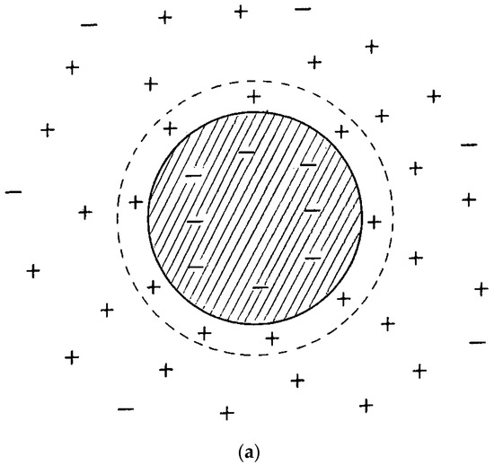
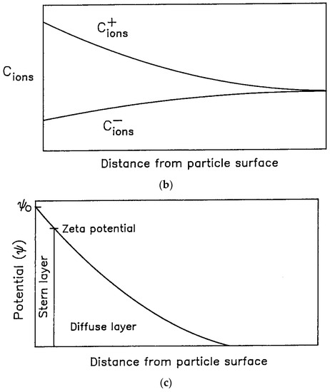
Figure 2.
Charged particle surrounded by an ionic cloud [9]. Variations of ionic concentration and electric potential are also shown. (a) Charged particle surrounded by an ionic cloud; (b) Variation of ionic concentration with distance from the particle surface; (c) Variation of electric potential with distance from the particle surface.
The suspensions of electrically charged particles are more viscous in comparison with the suspensions of neutral particles. The motion of fluid surrounding the charged particle distorts the electric charge cloud from its equilibrium state, resulting in additional stresses referred to as Maxwell stresses. The Maxwell stresses produced by the electrostatic attraction between the particle’s surface charge and the surrounding charge cloud of counter-ions hinder the motion of fluid inside the double layer and consequently an extra dissipation of energy takes place. This effect whereby additional stresses are produced and extra dissipation of energy takes place in a particulate fluid due to distortion of electrical double layers around the particles caused by fluid motion is called the “primary electroviscous effect”.
The rheology of suspensions of charged particles is investigated by a number of researchers [18,19,20,21,22,23,24,25,26,27,28]. The rheology of such suspensions is governed by a complex interplay of electrical, thermal, and viscous forces. The key factors to be considered are: the thickness of the electrical double layer with respect to the particle size, the distortion of the double layer from equilibrium due to fluid motion, and the resistance to fluid flow around the particle caused by electrical forces. For example, the viscosity of a suspension is expected to increase with the increases in the double layer thickness and electrical stress. Furthermore, shear-thinning is expected due to distortion of charge cloud around the particles caused by fluid motion.
The dimensional analysis indicates that four dimensionless groups are important, namely the Hartmann number (), the ion Peclet number (), the relative thickness of the electrical double layer (), and the dimensionless surface potential (). The definitions of these dimensionless groups are as follows:
where is surface potential (zeta potential), I is the bulk ionic strength defined as , is the valence of ionic species i, is the number density of ionic species i far away from the particle, is the total number of ionic species present in the fluid, is the ion diffusivity, ε is the permittivity of the fluid, is the Boltzmann constant, is the absolute temperature, is the particle radius, is the viscosity of fluid, e is the elementary electronic charge, is the shear rate, and is the Debye length defined as:
The electric Hartmann number is a measure of the ratio of electrical force to viscous force acting on the fluid. It represents rigidity of the charge cloud. Note that the diffusion of ions counteracts the Maxwell stresses and therefore, the Hartmann number includes the ratio of diffusion time to convection time of ions (see Equation (22)). The modification of the flow field around the particles caused by the electrostatic body force is small when << 1. When >> 1, the fluid adjacent to the particle experiences strong electrical forces and therefore, remains almost attached to the particle.
The ion Peclet number defined in Equation (23) measures the extent to which the motion of the fluid relative to the particle disturbs the charge cloud. For small ( << 1) the ionic atmosphere is distorted only slightly from its equilibrium shape because the diffusion of ions is strong as compared to convection of ions.
The dimensionless group defined in Equation (24) is the ratio of particle radius to Debye length . As the double layer extends a distance of from the surface of the particle, is a measure of the thickness of the electric double layer, relative to the particle size. If >> 1, the electric double layer is thin and if << 1, the electric double layer is thick.
The dimensionless surface potential () defined in Equation (25) is the ratio of electrical energy of ions to their thermal energy. When << 1, the number density of ions in the charge cloud differs only slightly from its value far away from the particle. In other words, the ion distribution in a fluid is affected only to a small extent near the particle surface, when a charged particle is introduced to the fluid.
When the distortion of charge clouds around the particles caused by fluid motion is small, that is, << 1, the constitutive equation for a dilute dispersion of electrically charged spherical particles can be expressed as:
where is the primary electroviscous coefficient which is, in general, a function of surface potential , Hartmann number , and double layer thickness (). The dispersion viscosity can be obtained from Equation (27) as:
Equation (28) could be re-cast in terms of the intrinsic viscosity as follows:
where
The primary electroviscous coefficient at low surface potential ( << 1) and low Hartmann number ( << 1) is given as [24]:
where f() is a power series function of with the two limiting forms as follows:
The form of f() given in Equation (32) is valid for small ( << 1), that is, thick double layers. The form of f() expressed in Equation (33) is valid for large ( >> 1), that is, thin double layers. For thin electrical layers ( >> 1), the primary electroviscous coefficient is given as:
whereas for thick electrical layers ( << 1), the coefficient reduces to:
Ohshima [29] has developed the following analytical expression for the primary electroviscous coefficient , valid for arbitrary surface potentials (no restriction on ), large ( >> 1), and Z-Z symmetrical type electrolyte where is the valence of the ion [29]:
where
In these equations, is the drag coefficient of ions, is the scaled ionic drag coefficient, is the Dukhin number [30], and . Using the relation (where is the ion diffusivity), it can be readily shown that:
For aqueous KCl solution at 25 °C, and [30]. For low surface potential and large , Equation (36) reduces to:
Assuming , Equation (40) in conjunction with Equation (39) leads to the expression for given by Equation (34).
Figure 3 shows the predictions of Equation (36) for different values of the double layer thickness . The electrolyte is KCl with and . The primary electroviscous coefficient decreases with the increase in (decrease in double layer thickness) for any given surface potential. Interestingly, the plot of versus for any given exhibits a maximum at some intermediate value of due to relaxation effect [29]. At high , reaches a nonzero limiting value of . It should also be noted that the value of where relaxation (peak) is observed increases slightly with the increase in .
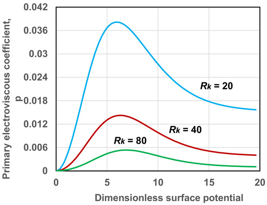
Figure 3.
Variation of primary electroviscous coefficient with dimensionless surface potential for different values of .
The electroviscous coefficient could be determined experimentally using viscosity measurements of dilute suspensions. Upon re-arrangement of Equation (29), one can write:
From the slope of versus data in the limit , one can determine the value of (and hence the primary electroviscous coefficient , see Equation (30)) experimentally. As an example, Figure 4 shows the plots of versus data for polystyrene latex suspensions consisting of negatively charged particles of diameter 250 nm [27]. The plots are shown for two different electrolyte (KCl) concentrations. As expected the experimental data exhibit a linear behavior with slopes of −. The intrinsic viscosity values for the data shown in Figure 4 are as follows: at KCl concentration of 4 × 10⁻⁵ M and at KCl concentration of 1.2 × 10⁻⁴ M. The corresponding values (primary electroviscous coefficient) are: 1.76 and 1.20, respectively.
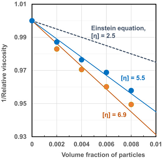
Figure 4.
Plots of versus data for polystyrene latex suspensions consisting of negatively charged particles of diameter 250 nm suspended in KCl solutions.
Figure 5 shows the variation of primary electroviscous coefficient with the electrolyte KCl concentration for two negatively charged monodisperse polystyrene latex suspensions [27]. The surface charge on the particles of more viscous latex suspension (top curve) was −6.85 μC/cm2 and the particle diameter was 106 nm. The surface charge on the particles of less viscous latex suspension (bottom curve) was −0.20 μC/cm2 and the particle diameter was 210 nm. With the increase in electrolyte concentration, the electrical double layer thickness decreases ( increases) and therefore, the coefficient decreases. For the same electrolyte concentration, the suspension of weakly-charged particles gives lower values, as expected. Furthermore, the value of the suspension of weakly-charged particles is also larger (hence thinner double layer) due to large particle size.
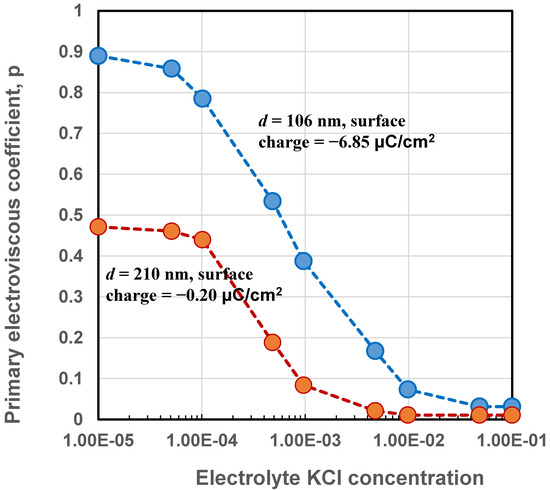
Figure 5.
Variation of primary electroviscous coefficient with electrolyte concentration for electrically charged polystyrene latex suspensions.
Thus far, our discussion about the primary electroviscous effect was largely restricted to small ( << 1). The ionic atmosphere around the particles was distorted only slightly from its equilibrium shape due to fluid motion. Russel [19] extended the work to arbitrary flow strengths (arbitrary ) and developed the following constitutive equation for dilute dispersions of charged spherical particles valid under conditions of thin double layer ( >> 1), small Hartmann number and low surface potential << 1. The full constitutive equation developed by Russel [19] for suspensions of electrically charged spheres is as follows:
where is the deviatoric stress tensor and is the Jaumann derivative. This constitutive equation predicts non-Newtonian shear-thinning behaviour of suspensions of electrically charged particles. Equation (42) gives the following expression for the suspension viscosity:
Thus the viscosity of dilute suspensions of electrically charged particles decreases with the increase in ion Peclet number . As an example, Figure 6 and Figure 7 show the variations of intrinsic viscosity of suspensions of charged particles with ion Peclet number . The plots are generated from Equation (43). As expected, the suspension exhibits shear-thinning in that the intrinsic viscosity decreases with the increase in the Peclet number. The versus plots exhibit with two distinct plateau regions: upper Newtonian plateau with high value when and lower Newtonian plateau with low value when . With the increase in the electrical double layer thickness, that is, decrease in , the intrinsic viscosity in the upper Newtonian region () increases at a fixed value of Hartmann number (see Figure 6). With the increase in the Hartmann number , the intrinsic viscosity in the upper Newtonian region () increases at a fixed value of the electrical double layer thickness (see Figure 7).

Figure 6.
Variation of [η] with Pe for suspensions of charged particles at different values of Hartmann number (Rk fixed at 8).
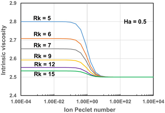
Figure 7.
Variation of [η] with Pe for suspensions of charged particles at different values of Rk (Ha fixed at 0.5).
Equation (42) also predicts that the dilute suspensions of electrically charged particles are viscoelastic in nature. It leads to the following expressions for the normal-stress differences in steady shearing flow:
Figure 8 shows the plots of first normal-stress difference as versus ion Peclet number for two different values of particle volume fraction. The first normal-stress difference increases initially with the increase in and then levels off at high . It also increases with the increase in particle volume fraction . The second normal-stress difference is plotted as versus in Figure 9. The second normal stress difference behaves in a manner similar to the first normal-stress difference.
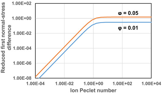
Figure 8.
Reduced first normal-stress difference as a function of ion Peclet number.
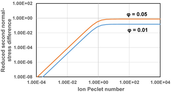
Figure 9.
Reduced second normal-stress difference as a function of ion Peclet number.
The constitutive equation developed by of Russel (Equation (42)) is valid for thin double layers ( >> 1), small Hartmann number, and low surface potential. Lever [22] has extended the analysis of Russel to thick double layers ( << 1) and conducted numerical calculations. The Hartmann number and surface potential were assumed to be small. His analysis shows that the suspension behaves as a non-Newtonian fluid with non-zero normal-stress differences and shear-thinning viscosity at high Peclet numbers when the charge cloud is deformed from equilibrium condition to a large extent.
Khair and Star [31] have considered the influence of particle surface charge on the bulk viscosity of dilute suspensions under the conditions of low surface potential, small Hartmann number, and gentle flow (small Peclet number). The bulk viscosity of a dilute suspension of electrically-charged spherical particles can be expressed as:
where is the primary bulk electroviscous coefficient. For thin electrical layers (>> 1), the primary bulk electroviscous coefficient is given as:
whereas for thick electrical layers ( << 1), the coefficient reduces to:
Figure 10 compares the bulk and shear primary electroviscous coefficients at a small Hartmann number of 0.1. The predictions of Equations (34) and (47) are compared for thin double layers ( >> 1) and the predictions of Equations (35) and (48) are compared for thick double layers ( << 1). Clearly, the bulk primary electroviscous coefficient is much higher than the shear primary electroviscous coefficient for the same electrical double layer thickness.
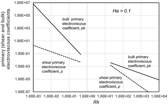
Figure 10.
Comparison of bulk and shear primary electroviscous coefficients at a small Hartmann number of 0.1.
5. Rheology of Suspensions of Rigid-Porous Spherical Particles
The rheology of dilute suspensions of porous rigid spherical particles is strongly dependent on the particle permeability. Zackrisson and Bergenholtz [32] have shown that the dipole strength of a porous rigid spherical particle immersed in an infinite matrix of incompressible Newtonian fluid is given as:
where and are defined as:
In Equation (50), is the permeability of particles. For impermeable particles, , , and consequently, the dipole strength given by Equation (49) reduces to that of solid spherical particles given by Equation (12). For completely permeable particles, , , and consequently, the dipole strength given by Equation (44) reduces to zero. The full constitutive equation for dilute suspensions of electrically-neutral porous rigid spherical particles can be expressed as follows:
where is the bulk stress tensor of the suspension and is the imposed or bulk rate of strain tensor on the suspension. According to Equation (52), the suspension is a Newtonian fluid with effective viscosity of η given as:
Equation (53) gives the following expression for the intrinsic viscosity of suspensions of electrically-neutral, porous, rigid and spherical particles:
Figure 11 shows the plot of intrinsic viscosity as a function of dimensionless permeability, defined as (note that ). The intrinsic viscosity decreases from a value of 2.5 corresponding to completely impermeable spheres () to a value of zero, corresponding to completely permeable spheres ().
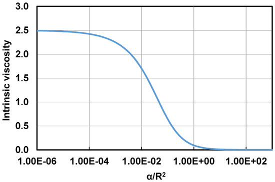
Figure 11.
Intrinsic viscosity as a function of dimensionless permeability ( ).
Natraj and Chen [33] have extended the analysis of the rheology of dilute suspensions of electrically-neutral porous spheres to electrically-charged spheres taking into consideration the primary electroviscous effect. According to the analysis presented by Natraj and Chen, the distortion of the charge cloud around the particles increases with the increase in the permeability of the particles leading to an increase in the intrinsic viscosity of suspension relative to intrinsic viscosity of suspension of uncharged porous particles. As an example, Figure 12 shows the plots of the ratio as a function of dimensionless permeability of particles for two different values of (ratio of particle radius to electrical double layer thickness). For any given plot, the Hartmann number is kept constant. Clearly the suspension of charged porous particles is more viscous as compared with suspension of uncharged porous particles for any given particle permeability. The enhancement of suspension viscosity due to primary electroviscous effect becomes more intense with the increase in particle permeability.
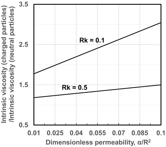
Figure 12.
Influence of particle permeability on the intrinsic viscosity of suspension of electrically-charged porous particles.
6. Rheology of Suspensions of Non-Rigid (Soft) Solid Particles
Particulate fluids consisting of deformable solid particles exhibit non-Newtonian behavior [9,34,35]. In shear flow, they exhibit shear-thinning and normal-stress effects. In uniaxial elongational flow, the strain-thickening effect is observed. In simple shear flow, the initially spherical particle deforms into an ellipsoid of fixed dimensions and orientation at a given shear rate. The material inside the ellipsoidal particle undergoes continuous deformation and rotation (tank-treading motion) The rheology of suspensions of particles composed of deformable purely elastic material (Hookean solid), with elastic modulus of , depends on the following dimensionless group:
is the ratio of viscous stress which tends to elongate and orient the particles in the direction of flow to elastic stress which tends to recover the original shape of the particles. When << 1, the suspension is more viscous as the elastic force dominates and the particles are nearly spherical. When >> 1, the suspension becomes less viscous as viscous stresses now dominate and the particles become elongated and oriented in the direction of flow.
Goddard and Miller [34] calculated the dipole strength of soft purely elastic particles immersed in an infinite matrix of incompressible Newtonian fluid for weakly time-dependent flows. Their expression for could be expressed as follows:
where refers to the symmetric and traceless part of the indicated tensor. From Equations (8) and (56), it follows that:
Note that for a dilute suspension, the rate of strain tensor far away from the particle can be equated to the bulk or imposed rate of strain tensor on the suspension. Equation (57) could be further approximated as [9]:
Equation (58) predicts non-Newtonian behavior of dilute suspensions of deformable purely elastic solid particles. It gives the following expressions for the relative shear viscosity and reduced normal stresses when the suspension is subjected to steady shearing flow:
where is the dimensionless group defined in Equation (55), is the first normal stress difference and is the second normal stress difference. From Equation (59), it follows that the intrinsic viscosity of a suspension of soft elastic solid particles is:
It may be of interest to note that Roscoe [35] presented a similar set of equations for dilute suspensions of viscoelastic solid-like particles (Kelvin-Voigt type solid particles). In the case of purely elastic solid particles, the equations presented by Roscoe [35] reduce to the equations presented here (Equations (59)–(62)).
Figure 13 shows the plot of intrinsic viscosity as a function of . The intrinsic viscosity decreases with the increase in indicating that suspension of soft elastic particles is shear-thinning in nature. It should also be noted that at high ( > 1), the intrinsic viscosity becomes negative indicating that the viscosity of suspensions of soft elastic particles decreases with the increase in particle concentration at high . According to Equation (54), the relative viscosity of suspension becomes equal to () at high . The reduced normal stress differences are plotted in Figure 14 and Figure 15 as (Figure 14) and (Figure 15) versus . The reduced normal stress differences increase initially with the increase in , reach some maximum values, and then decrease with further increase in .
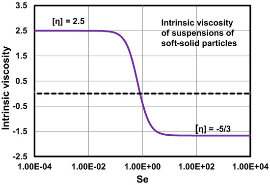
Figure 13.
Intrinsic viscosity as a function of for suspensions of soft solid particles.
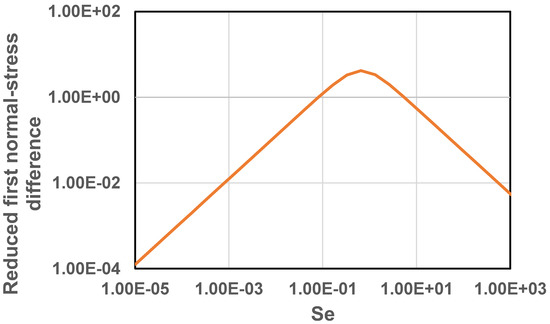
Figure 14.
Reduced first normal-stress difference as a function of for suspensions of soft-solid particles.
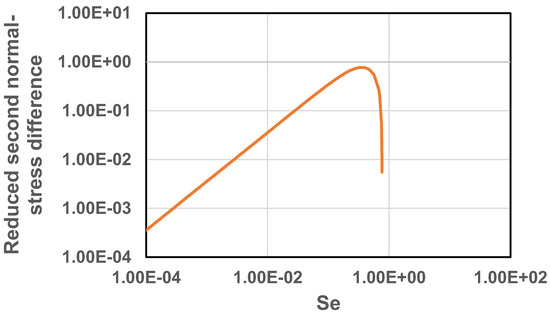
Figure 15.
Reduced second normal-stress difference as a function of for suspensions of soft-solid particles.
The constitutive equation expressed in the form of Equation (58) also predicts strain-thickening behavior in uniaxial elongational flow, that is, the elongational viscosity () increases with the increase in the elongation rate () as indicated by the following equation:
Finally, it should be realized that the Goddard and Miller analysis [34] and therefore the Equations (58)–(63) assume infinitesimal deformation of particles. Thus the plots shown in Figure 13, Figure 14 and Figure 15 are strictly valid for . Little or no experimental data are available to verify these theoretical predictions. However, a number of interesting analytical and numerical studies have been published recently extending the works of Goddard and Miller [34] and Roscoe [35] to arbitrarily large deformations [36,37,38,39,40,41]. Furthermore, Gao et al. [38] have considered the effect of the initial particle shape of elastic particles (usually assumed to be spherical) on the motion and rheology of elastic particles in a shear flow. While the initially-spherical elastic particles exhibit the well-known “tank-treading” motion in shear flow, the initially-ellipsoidal elastic particles exhibit so-called “trembling motion” in that they tend to oscillate without making a full rotation. As the initial shape of the particle becomes more elongated, the elastic particles undergo “tumbling motion” similar to that of rigid ellipsoidal particles in a shear flow.
7. Rheology of Emulsions
Emulsions are dispersed systems consisting of droplets of one liquid distributed throughout another immiscible liquid. Emulsions exhibit non-Newtonian rheology due to deformation and orientation of droplets in a flow field [9,42,43,44,45]. The shape and orientation of droplet with respect to the flow direction is governed by two dimensionless groups: the viscosity ratio λ, defined as the ratio of droplet fluid viscosity () to continuous-phase viscosity (), and the capillary number , defined as:
where is the shear rate, is the radius of the un-deformed droplet, and is the interfacial tension between the two immiscible liquids. There is competition between the hydrodynamic stress which tends to stretch the droplet and the interfacial stress which tends to contract the droplet into a sphere. With the increase in the capillary number, the droplet becomes more elongated and oriented with the flow direction. Due to this elongation and orientation of droplets emulsions exhibit shear-thinning behavior. Other non-Newtonian characteristics exhibited by emulsions are (i) non-zero normal stresses in shear flow and (ii) strain-thickening in extensional flows.
Assuming droplets to remain nearly spherical in shape, that is, , Taylor [46] developed the following expression for the dipole strength of a droplet immersed in an infinite matrix of incompressible Newtonian fluid:
where is the ratio of dispersed-phase viscosity to continuous-phase viscosity. The constitutive equation for the dilute emulsion in the limit can be obtained from Equations (8) and (65) as follows:
Thus the effective viscosity of a dilute emulsion in the limit turns out to be
Equation (67), referred to as the Taylor equation, reduces to the Einstein equation, Equation (15), in the limit . From Equation (67), the intrinsic viscosity of an emulsion is as follows:
Figure 16 shows the plots of relative viscosity versus droplet concentration for dilute emulsions for different values of the viscosity ratio . The plots are generated using the Taylor equation, Equation (67). With the increase in , the slope of the plot, that is , increases. When , the slope is 2.5 and the droplets behave as rigid particles. When , the slope is 1.0 and the droplets behave as bubbles. Thus the relative viscosity of emulsions can be manipulated by varying the viscosity ratio while keeping all the other compositional variables constant. One possible way to manipulate the viscosity ratio, and hence the relative viscosity, in practical emulsions is to vary the temperature of the emulsion [47] provided that the temperature-dependence of viscosity is different for the two liquids involved.
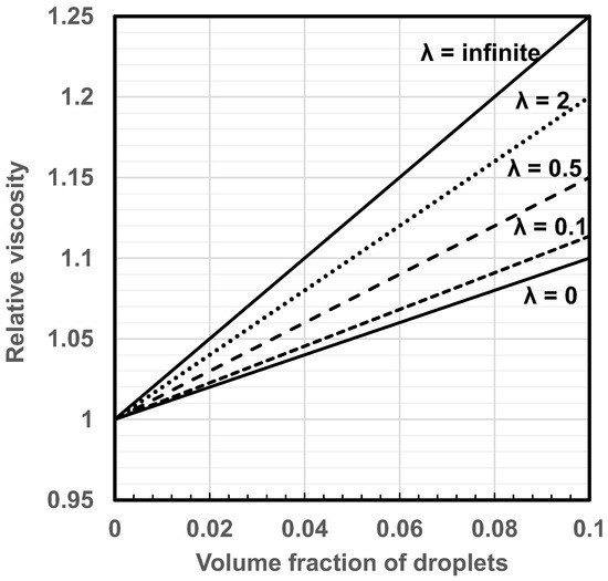
Figure 16.
Relative viscosity versus droplet concentration for dilute emulsions for different values of the viscosity ratio .
Figure 17 shows comparison between experimental viscosity data and theoretical predictions. The emulsions tested are toluene-in-glycerol [48] with viscosity ratio of 8.66 × 10⁻⁴. The emulsions are produced by mixing the two liquids in an agitated vessel at different agitator speeds. The intrinsic viscosity (Equation (68)) of these emulsions is 1.0013. The experimental data show good agreement with the Taylor viscosity equation when . At higher concentrations of dispersed-phase, the Taylor equation under predicts the emulsion viscosity.
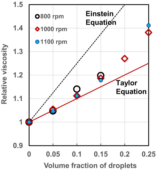
Figure 17.
Comparison between experimental viscosity data and theoretical predictions for emulsions.
The constitutive equation of a dilute emulsion expressed in the form of Equation (66) does not predict non-Newtonian rheology of emulsions as deformation of droplets is neglected and . Schowalter et al. [42] and Frankel and Acrivos [43] extended the work of Taylor [46] by considering the first-order deformation of droplets and developed the following equation for the dipole strength of a droplet immersed in an infinite matrix of incompressible Newtonian fluid:
From Equations (8) and (69), it follows that:
where has been equated to the imposed rate of strain tensor on the emulsion.
According to Frankel and Acrivos [43], Equation (70) could be recast as:
where is the deviatoric stress tensor and is the characteristic time constant of the emulsion given as:
Equation (71) predicts shear-thinning in emulsions in steady-shear flows and leads to the following expression for the shear viscosity [9] of dilute emulsions:
Based on Equation (73), the intrinsic viscosity of an emulsion can be expressed as:
where and is the capillary number (defined in Equation (64)). Thus intrinsic viscosity of an emulsion depends on viscosity ratio and capillary number . In the limit , Equation (74) reduces to Equation (68). Figure 18 shows the plots of intrinsic viscosity generated from Equation (74). At low values of capillary number ( < 0.1), the intrinsic viscosity is always greater than or equal to 1, regardless of the viscosity ratio, indicating that the addition of droplets always increases the viscosity of emulsion due to interfacial tension effect. At high capillary numbers where the interfacial tension effect is negligible, the intrinsic viscosity is non-zero positive only if the viscosity ratio is larger than 1. When , the intrinsic viscosity is zero at high capillary numbers indicating that the addition of droplets has no effect on the viscosity of emulsion. When , the intrinsic viscosity is negative at high capillary numbers indicating that the addition of droplets results in a decrease in the viscosity of emulsion.

Figure 18.
Intrinsic viscosity of emulsion as a function of capillary number for different values of viscosity ratio .
The Frankel and Acrivos equation, Equation (71), also predicts non-zero normal stress differences in shear flow of dilute emulsions. Equation (71) leads to the following expressions for the normal stress differences:
The plots of normal stress differences for emulsions are shown in Figure 19 and Figure 20. In Figure 19, the first normal stress difference is plotted as versus , keeping . In Figure 20, the second normal stress difference is plotted as versus , keeping . The normal stress differences increase initially with the increase in due to interfacial-tension related elasticity of droplets. After reaching a certain maximum value, the normal stress differences fall off sharply with further increase in . The decrease in the magnitude of the normal stress differences at high is expected as viscous stresses dominate over the restoring interfacial stresses at high .

Figure 19.
Reduced first normal stress difference versus , keeping .
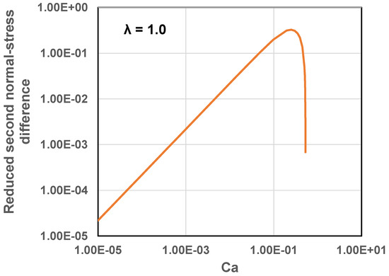
Figure 20.
Reduced second normal stress difference versus , keeping .
According to the Frankel and Acrivos equation, Equation (71), the emulsions behave as strain-thickening in uniaxial elongation flows as indicated by the following expression of elongation viscosity obtained from Equation (71):
Finally it should be pointed out that the Frankel and Acrivos analysis and therefore the Equations (69)–(77) assume infinitesimal (first order) deformation of droplets. Thus the plots shown in Figure 18, Figure 19 and Figure 20 are strictly valid for small deformation of droplets corresponding to . Wetzel and Tucker [39] have extended the small deformation analysis to arbitrary deformations for dispersions with unequal viscosities and zero interfacial tension.
7.1. Influence of Electric Charge Present on the Surface of Emulsion Droplets
Ohshima [29] has studied the influence of droplet surface charge on the rheology of dilute emulsions. The relative viscosity of dilute emulsions of electrically charged droplets at low capillary numbers can be expressed in the following modified-form of the Taylor viscosity equation (Equation (67)):
where is the primary electroviscous coefficient. Ohshima [29] has developed a general expression for valid under the following conditions: arbitrary surface potential, arbitrary electric double layer thickness , weak flow (small Peclet number) such that the charge cloud around the droplet is disturbed from equilibrium state only slightly, and small capillary number so that the droplets remain spherical. For large () and arbitrary surface potential, the expression for of emulsions reduces to [29]:
where is the scaled ionic drag coefficient, defined in Equation (37). In the limit , Equation (79) gives as expected for the uncharged droplets. For very thin double layer () and high surface potential , approaches a nonzero limiting value given by:
If we substitute this expression of into Equation (78), the Einstein viscosity equation, Equation (18), for dilute suspensions of uncharged rigid-solid spheres is recovered. This implies that emulsion droplets with thin double layers and very high surface potentials behave like uncharged rigid-solid spheres regardless of the viscosity ratio . This phenomenon is referred to as “solidification effect” in the literature [29].
Figure 21 shows the plots of versus for different values of viscosity ratio . The plots are generated using Equation (79). The matrix is assumed to be an aqueous KCl solution. As expected, increases initially with the increase in surface potential and then levels off at high surface potentials. With the increase in the viscosity ratio, the primary electroviscous coefficient of emulsion decreases.

Figure 21.
Primary electroviscous coefficient versus for different values of viscosity ratio .
As , , indicating that the influence of interface becomes less and less important with the increase in the viscosity ratio.
7.2. Influence of Surfactant on Emulsion Rheology
In the preceding discussion, it was observed that dilute emulsions of electrically-neutral droplets exhibit Newtonian behavior when and the droplets are spherical. The emulsions exhibit shear-thinning and elastic behavior (non-zero normal stress differences) only when and the droplets undergo significant deformation. It is interesting to note that dilute emulsions can exhibit non-Newtonian rheology even in the absence of any deformation, that is, when and the droplets are spherical [49,50,51]. The additional mechanism of non-Newtonian behavior in emulsions comes into play when surfactant molecules are present at the surface of droplets. The flow of continuous-phase fluid around the droplet results in non-uniform concentration of surfactant at the droplet surface. The resulting inhomogeneity in surfactant concentration at the droplet surface generates Marangoni stress due to interfacial tension gradient. The Marangoni stress results in a jump in tangential viscous traction across the droplet interface. Due to inhibition of the transmission of tangential stresses from the continuous-phase fluid to the droplet fluid, the droplets tend to behave more like solid particles.
The dimensionless group that determines the rheology of dilute emulsion of surfactant covered droplets when is the Marangoni number . Blawzdziewicz et al. [49] define as:
where ( is interfacial tension in the absence of surfactant and is equilibrium interfacial tension in the presence of surfactant at the droplet surface). At low shear rates (high ), the Marangoni stress dominates over the viscous stress and therefore, the emulsion droplets behave more like rigid particles. Consequently the emulsion viscosity is relatively high. At high shear rates (low ), the viscous stress dominates over the Marangoni stress resulting in lower emulsion viscosity.
The Marangoni number defined in Equation (81) is relevant when the surfactant is non-diffusing type. When diffusion of surfactant is important, the dimensionless group that governs the rheology of emulsions is given as follows [51]:
where is the Gibbs elasticity of the interface and is the effective diffusion coefficient of surfactant. As diffusion of surfactant molecules counteracts the Marangoni-stress, the dimensionless group (modified Marangoni number) includes the ratio of diffusion time to convection time of surfactant molecules. When the diffusion of surfactant molecules is very fast, that is is large, is very small and therefore, the effect of interface elasticity on emulsion rheology can be neglected.
In gentle flows (small Peclet number, small capillary number), the effective viscosity of a dilute emulsion can be expressed as [52]:
where is the interfacial-rigidity parameter, defined as:
The interfacial-rigidity parameter varies from 0 to 1. When the interface is completely rigid, and Equation (83) becomes the Einstein viscosity equation for suspensions of rigid-solid particles (Equation (15)). The interface is completely mobile () when and , that is, the droplet has zero viscosity and the interface has negligible elasticity. The interface is completely rigid and the interfacial-rigidity parameter is 1, under the following conditions: (a) , that is, the interface possesses high Gibbs elasticity (note that when , is 1 regardless of the droplet to matrix viscosity ratio) and (b) , that is, the viscosity ratio is very high (note that when , is 1 regardless of the degree of elasticity of the interface). The plots of versus for different values of the viscosity ratio are shown in Figure 22.
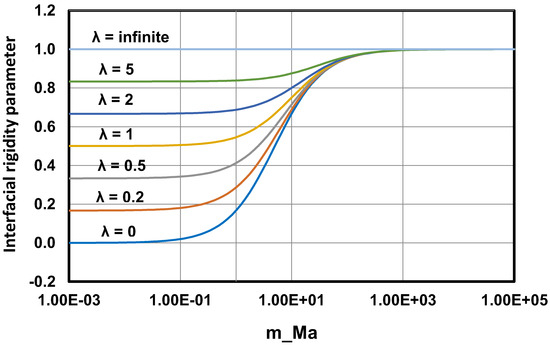
Figure 22.
Plots of versus for emulsions for different values of the viscosity ratio .
In the viscosity expression given in the form of Equations (83) and (84), it is assumed that the interface dilational and shear viscosities are negligible. In the presence of surfactant or other additives at the interface, the interfacial viscosities may not be negligible. In order to account for the interfacial viscosities, the interfacial-rigidity parameter needs to be modified as follows [9]:
where is the shear Boussinesq number and is the dilational Boussinesq number. The Boussinesq numbers are dimensionless groups defined as:
where and are interfacial shear and dilational viscosities, respectively.
Figure 23 show the plots of versus for different values of the interfacial viscosity term . The interfacial elasticity term is kept zero. Clearly the interfacial rigidity parameter increases with the increase in the interfacial viscosities. The effect of interfacial viscosities on is more at low values of the viscosity ratio . At high values of , is 1 regardless of the magnitude of the interfacial viscosities.
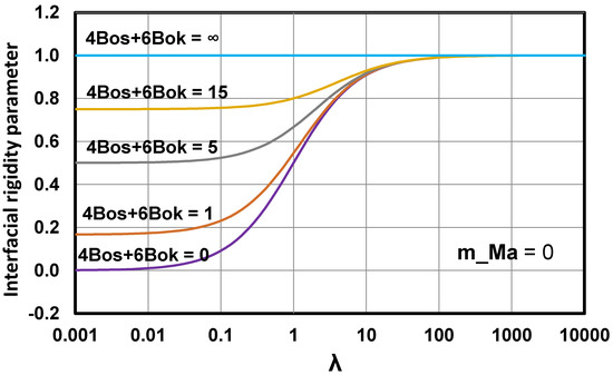
Figure 23.
Plots of versus for different values of the interfacial viscosity term .
8. Rheology of Bubbly Suspensions
In gentle flows (low Reynolds number, low capillary number), the rheological constitutive equation for a dilute suspension of spherical bubbles can be expressed as:
where is the bulk viscosity of suspension and is the shear viscosity of suspension. The expressions for and for dilute suspensions of electrically-neutral bubbles, in the absence of any additives present at the interface, are given as follows:
When the bubbles are electrically-charged or when additives (such as surfactant) are present at the interface, the above expressions for and need to be modified.
8.1. Influence of Electric Charge Present on the Surface of Bubbles
Both shear viscosity of suspension and bulk viscosity of suspension are affected by the presence of electric charge on the surface of the bubbles. For dilute suspensions of electrically-charged bubbles in incompressible Newtonian fluids, the shear and bulk viscosities are given as [31]:
where is the primary shear electroviscous coefficient and is the primary bulk electroviscous coefficient. Under the conditions of very thin double-layers (), Z-Z symmetrical type electrolyte, and arbitrary surface potentials (no restriction on ), the primary shear electroviscous coefficient is given by the following expression [29]:
At high surface potentials, Equation (93) gives of 3/2. Under the conditions of low surface potential, small Hartmann number, and small Peclet number, the primary bulk electroviscous coefficient is given as [31]:
It is interesting to note that both and approach a zero value for suspensions of rigid particles with very thin double layers (). However, in the case of bubbles or droplets with very thin double layers (), both and approach non-zero values at high surface potentials. One possible reason for this is that the relative fluid velocity on the surface of the rigid particles is vanishingly small (no-slip condition) as compared with the relative fluid velocity on the mobile surfaces of bubbles or droplets [31]. The electroviscous stress in the thin double layers is expected to be small when the fluid velocity relative to the particles is small in that region.
8.2. Influence of Surfactant Present on the Surface of Bubbles
When surfactant is present on the surface of the bubbles, the interfacial shear and dilational viscosities may be significant enough to affect the bulk rheology of bubbly suspensions. In addition to interfacial viscosities, the interfacial elasticity (Marangoni effect) may also have a significant influence. The effective shear viscosity of dilute bubbly suspensions in the presence of non-zero interfacial viscosities and elasticity is given by Equation (83) with the following expression for the interfacial-rigidity parameter :
The bulk viscosity of a dilute bubbly suspension with non-zero interfacial dilational viscosity is given as [9,53]:
where is the radius of the bubble.
8.3. Influence of Capillary Number
The preceding discussion on the rheology of dilute bubbly suspensions was restricted to weak flows characterized by a small capillary number (). The bubbles were assumed to be spherical in shape. At high capillary numbers, the bubbles become elongated and oriented with the flow direction. Consequently, the bubbly suspensions exhibit non-Newtonian rheology including shear-thinning and non-zero normal stress differences.
The full rheological constitutive equation for dilute bubbly suspensions, when bubbles undergo first-order deformation, is given as follows:
In steady shear flow, Equation (98) leads to the following expressions for relative viscosity and reduced normal-stress differences [54,55]:
In uniaxial elongation flows, the bubbly suspensions behave as strain-thickening as indicated by the following expression of elongation viscosity obtained from Equation (98):
9. Rheology of Suspensions of Capsules
Capsules are droplets of liquid covered with a thin, deformable, elastic-solid membrane [9,56]. The motion and deformation of capsules and the rheology of dilute suspensions of capsules has been studied extensively by Barthes-Biesel and co-workers [56,57,58,59,60,61,62,63,64,65,66,67,68,69,70,71,72,73,74,75,76]. In shear flow, capsules behave differently from rigid-solid particles and liquid droplets. At low shear rates, capsules act as rigid-solid particles and rotate as a rigid body regardless of the viscosity of the enclosed liquid. However, at high shear rates, the capsules behave more like liquid droplets in that they deform and attain a steady-state orientation. The main difference between the behaviors of capsules and droplets at high shear rates is that the thin elastic-solid membrane covering the surface of the capsules undergoes tank-treading motion whereas no such membrane exists on the surface of the droplets. The liquid present inside the capsules also undergoes internal circulation induced by tank-treading motion of the membrane.
The rheology of suspension of capsules is strongly dependent on the instantaneous shape and orientation of the capsules (assumed spherical initially) covered with thin elastic-solid membranes. The time evolution of the capsule shape and orientation is specified by two second-order symmetric and traceless tensors and where specifies the radial displacement of the material points of the membrane and specifies the tangential in-plane displacement of the material points of the membrane. Both and depend on the mechanical properties of the membrane as well as the imposed flow field. The mechanical behavior of the membrane material (assumed to be isotropic and purely elastic) is specified by a strain energy function defined as internal strain energy per unit of initial membrane area. For small deformations, can be expressed in the following form [58]:
where is the membrane surface elastic modulus, and are extension ratios along the principal directions, and are material elastic coefficients depending on the type of membrane. In the literature on capsules, the following two types of membranes are often mentioned: MR (Mooney-Rivlin) type membrane and RBC (red blood cells) type membrane. The MR type membrane is made up of an infinitely thin sheet of isotropic, volume-incompressible elastomer, with the following values of :
The RBC type membrane is made up of a lipid bilayer lined with a protein network that imparts elasticity to the membrane. The RBC type membrane is easily shearable but offers considerable resistance to any increase in local surface area, and has the following values of :
The time evolution of the deformation tensors and is given as:
where is the capsule capillary number defined as , is the Jaumann derivative, and are symmetric and traceless tensors which are linear functions of deformation tensors and , and , are viscosity-ratio dependent parameters. The tensors and as well as the parameters , are given below:
The dipole strength of a single capsule located in an infinite matrix fluid has been determined by Barthes-Biesel and Rallison [58] by considering first-order (small) deformation of capsule. The expression for is as follows [9,58]:
Therefore, the rheological constitutive equation for a dilute suspension of identical capsules in a Newtonian matrix fluid can be expressed as (see Equation (8)):
In steady simple shear flow,
For MR type membranes, the expressions for and are as follows:
where
For RBC type membranes, the expressions for and are as follows:
From Equation (116), it can be readily shown that the effective viscosity of a dilute suspension of capsules with MR type membranes is as follows:
where
Based on Equation (129), the limiting intrinsic viscosities of suspension of capsules (with MR type membranes) at low and high capillary numbers are as follows [9]:
For dilute suspensions of capsules with RBC type membranes, Equation (116) leads to the following expression for the effective viscosity:
Based on Equation (133), the limiting intrinsic viscosities of suspension of capsules (with RBC type membranes) at low and high capillary numbers are as follows [9]:
10. Rheology of Suspensions of Core-Shell Particles
10.1. Solid Core—Porous Shell
The rheology of dilute suspensions of solid core—porous shell particles has been investigated by Zackrisson and Bergenholtz [32]. The solid core—porous shell particles simulate sterically-stabilized soft particles consisting of solid core and a hairy polymer and/or surfactant coating. The dipole strength of a single electrically-neutral solid core—porous shell particle immersed in an infinite matrix of Newtonian incompressible fluid can be expressed as follows [9,32,77]:
where is the radius of the solid core, is the radius of the composite core-shell particle, is defined in terms of the permeability () of the porous shell as: , and and are given as:
It should be pointed out that in the physical chemistry literature where sterically-stabilized particles (solid core—porous shell particles) are widely discussed [77], the friction coefficient is used, instead of permeability . The friction coefficient is related to permeability as and therefore .
Using Equation (136), the constitutive equation for dilute suspensions of solid core—porous shell particles can be expressed as:
From Equation (139), it follows that:
For impermeable shells, and and therefore, the core-shell particles behave as hard spheres with . When and , the porous shell vanishes and ; in this case, the suspension consists of hard particles of radius .
Ohshima [77] has studied the influence of primary shear electroviscous effect on the viscosity of dilute suspensions of soft particles. Soft particles are solid core—porous shell particles where a solid core particle is covered with an ion-penetrable surface layer of polyelectrolytes (porous shell). The polyelectrolyte layer consisted of uniformly distributed charged groups of valence Z. The charge density of the immobile charges (fixed on the polyelectrolyte chains) is where is the density of charged groups in the polyelectrolyte layer. The core particle surface is assumed to be uncharged. The effective viscosity of dilute suspensions of such soft particles is given as:
Under the condition of low fixed charge density (low ), the primary electroviscous coefficient can be expressed as [77]:
where is the valence of the ionic species i, is the drag coefficient of ionic species i, and is the surface potential at the outer surface of the porous layer () given as:
The expression for under the restrictions is as follows:
Figure 24 shows the plots of versus for two different values of . The value of is fixed to be 75. Interestingly (and hence ) exhibits a minimum at a certain value of and the minimum shifts to higher with the increase in . No such minimum is observed in suspensions of electrically charged hard spheres.
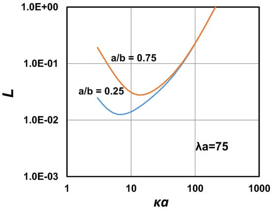
Figure 24.
Plots of versus for two different values of .
10.2. Solid Core—Liquid Shell
The rheology of dilute suspensions of solid core—liquid shell particles in another immiscible liquid was investigated by Davis and Brenner [78]. Let the solid core be of radius and the outer liquid shell be of thickness of . Let the viscosities of the shell and matrix liquids be and , respectively. Assuming negligible deformation of the liquid shell, Davis and Brenner [78] obtained the following expression for the dipole strength of a single solid core-liquid shell particle immersed in an infinite matrix of Newtonian incompressible fluid:
where is a dimensionless function of viscosity ratio and radii ratio (), and is the rate of deformation tensor far away from the particle. The function is given as follows:
Using the expression for the dipole strength (Equation (146)), the rheological constitutive equation for a dilute suspension of identical spherical particles of solid-core—liquid shell type can be expressed as:
From Equation (148), the relative viscosity of dilute suspension is:
When , Equation (147) gives and Equation (149) reduces to the Einstein viscosity equation for dilute suspensions. When , the solid core vanishes, and Equation (149) reduces to the Taylor viscosity equation for dilute emulsions.
10.3. Liquid Core—Liquid Shell
Liquid core—liquid shell particles are also referred to as double emulsion droplets. Let the inner core drop be of radius and the outer liquid shell be of thickness . Let the viscosity of the continuous-phase fluid be , the viscosity of the outer shell liquid be , and the viscosity of the inner core liquid be .
Assuming negligible deformation of double emulsion droplet, Stone and Leal [79] determined the velocity and pressure distribution interior and exterior to the globule. They also determined the following expression for the dipole strength of a single double-emulsion droplet located in an infinite matrix fluid:
where is a dimensionless function of viscosity ratios and , and radii ratio (), given as:
The coefficients depend on and are given as:
Using the expression for (Equation (150)), it can be readily shown that the rheological constitutive equation for a dilute suspension of identical spherical double-emulsion droplets is given by:
From Equation (156), it follows that the relative viscosity of a dilute suspension of double-emulsion droplets is:
When the outer shell liquid of double-emulsion droplets is very viscous (), and consequently Equation (157) reduces to the Einstein viscosity equation for dilute suspensions of rigid spheres. When , and therefore, Equation (157) reduces to the Taylor viscosity equation for dilute emulsions. It should also be noted that double emulsion droplets with very thin outer shells behave like rigid particles regardless of the viscosities of the inner core liquid and shell liquid.
11. Rheology of Suspensions of Rigid Non-Spherical Particles
The rheological behavior of suspensions of rigid non-spherical particles has been studied extensively [8,9,10,80,81,82,83,84,85,86,87,88,89,90,91,92,93,94,95,96,97,98,99,100,101,102,103,104,105,106,107,108,109,110,111,112,113,114,115,116,117,118,119,120,121,122,123,124,125,126,127,128,129,130]. The rheology of dilute suspensions of non-spherical particles (assumed axially symmetric) is strongly dependent on the shape, aspect ratio (length of particle along its axis of symmetry to its length perpendicular to the axis of symmetry), and orientation distribution function of particles. Let be a unit vector parallel to the axis of symmetry of particle (and locked into the particle) that specifies the orientation of the particle. Let be the orientation distribution function of particles that specifies the orientation state of the particles present in the suspension at any time . The orientation distribution function could be interpreted in two ways: (a) the probability that a particle is oriented in a neighborhood of at time is given by ; and (b) the fraction of the total number of particles in the suspension with orientations lying between and at any time is given by . Let be the dipole strength of a reference particle with orientation , located in an infinite matrix fluid. Therefore, the average dipole strength of a dilute suspension can be expressed as:
Thus the calculation of the average dipole strength, and hence the bulk stress, of a dilute suspension of non-spherical particles requires the knowledge of the orientation distribution function . Assuming that particles undergo rotary Brownian motion, the orientation distribution function of suspension can be obtained from the solution of the following Fokker-Planck equation in space:
where refers to divergence and is the rotary diffusivity of particles.
The average dipole strength of a dilute suspension of identical non-spherical particles, defined in Equation (158), is related to the rate of deformation tensor of suspension as follows:
where is the volume of a particle, and are shape factors dependent on the particle aspect ratio. The second and fourth moments of are defined as:
Using Equations (7) and (160), the rheological constitutive equation of a dilute suspension of identical non-spherical particles can be written as [9]:
For long thin rod-shaped particles (), the shape factors and are as follows:
For flat circular disk-shaped particles (), the shape factors and are as follows:
Let us now consider two different cases: Case A where the axisymmetric non-spherical particles of the suspension are large enough to ignore the rotary Brownian motion, that is, the particles are non-Brownian (); and Case B where the axisymmetric non-spherical particles are small enough that the rotary Brownian motion is significant, that is, the non-spherical particles are Brownian ().
Case A: When non-Brownian axisymmetric particles are subjected to shear flow, they undergo rotational motion in fixed orbits, referred to as Jeffery orbits. Each particle rotates in a fixed orbit. The distribution of particles in different orbits is determined by the initial orientation state of the particles at . Assuming that all the particles of the suspension are identical, each particle possesses the same period of rotation given as [9]:
where is the aspect ratio and is the shear rate. In this case, the orientation distribution function of particles is periodic in nature. As the bulk stress depends on the orientation state of particles, the rheological properties are also periodic functions of time. For example, the instantaneous intrinsic viscosity of suspension is small during that portion of the time period when the particles are aligned with the flow field, and is large during that portion of the time period when the particles are not aligned with the flow field, that is, the intrinsic viscosity oscillates with time period . With the increase in shear rate , the time period decreases and the rheological properties oscillate at a faster rate. Interestingly, the rheological properties of a suspension of identical, non-Brownian and non-spherical particles, are indeterminate if the initial orientation state of the particles, specified by at , is not known. Note that at if the particles are initially randomly oriented.
Case B: Small particles (particles with their largest dimension less than a few microns) undergo both translational and rotational Brownian diffusion, that is, random translational displacement and random angular displacement. However, it is only the rotary Brownian motion that affects the rheology of suspensions of non-spherical particles. The rotary Brownian motion affects the flow behavior of suspensions of non-spherical particles in two ways: (i) it alters the angular velocity of the particles. This is referred to as direct effect of Brownian motion on the rheology of suspension. The bulk stress, and hence rheological properties, of suspension are sensitive to the angular velocity of particles. Consequently a change in the angular velocity of particles due to rotary Brownian motion produces a corresponding change in the rheological properties of suspension. An important point to note is that the direct effect of rotary Brownian motion on suspension rheology is present even in the absence of imposed macroscopic motion, that is, even when , and is often referred to as diffusion stress; and (ii) the rotary Brownian motion also affects the orientation distribution function . It tends to randomize the orientations of the particles. This is referred to as indirect effect of Brownian motion on suspension rheology. Interestingly, the bulk stress (and hence rheological properties) of suspension in the presence of rotary Brownian motion is determinate under all conditions, regardless of the initial orientation state of the particles. If sufficient time is allowed, the orientation distribution reaches a unique steady state value that is independent of the initial orientation state of particles. It should be noted that the particles still rotate but not in fixed orbits. There is no equilibrium orientation of particles. Only is stationary in time indicating that for any orientation as many particles leave the neighborhood of as enter it. Interestingly, the dilute suspensions of non-spherical Brownian particles exhibit shear-thinning and normal-stresses when subjected to simple shear flow. The rotary Brownian motion tends to randomize the orientations of the particles whereas the viscous stresses tend to orient the particles such that they are least disruptive to flow. Thus the steady state value of the orientation distribution function varies with the rotary Peclet number, defined as . At low values of , the viscosity of suspension is high as Brownian motion dominates and the particles are randomly oriented. At high values of , the viscous stresses dominate over the Brownian motion and the particles become aligned with the flow resulting in lower viscosity of suspension.
Chen and Koch [131] have explored the influence of particle electric charge on the rheology of dilute suspensions of Brownian rod-shaped particles (charged fibers) with large aspect ratio under the conditions of small Hartmann number and thick double layer ( particle radius). The presence of electric charge on the particles leads to three additional contributions to the bulk stress of suspension: two direct effects and one indirect effect. One direct effect comes from the distortion of electrical double layer when the suspension is subjected to macroscopic motion. The motion of fluid surrounding the charged particle distorts the electric charge cloud from its equilibrium state, resulting in an electrical stress. Interestingly, the distortion of electrical charge cloud also results in an electric torque on the particle. The electric torque on the particle affects the angular velocity of the particles. This is the second direct effect of electric charge on the bulk stress of suspension. The electric torque on the particles also affects the orientation distribution function of particles. This is the indirect effect of electric charge on the rheology of suspensions.
12. Rheology of Suspensions of Ferromagnetic Particles
Suspensions of ferromagnetic particles are referred to as ferrofluids in the literature [132]. A number of studies have been published on the mechanics, rheology, and applications of ferrofluids [132,133,134,135,136,137,138,139,140,141,142,143,144,145,146,147,148,149,150,151,152,153,154,155,156,157,158,159,160,161,162,163,164,165,166,167,168]. The particles of ferrofluids are usually small in size (about 10 nm in diameter) and are made up of some ferromagnetic material such as iron oxide. The atoms of ferromagnetic materials possess a net magnetic dipole moment due to the presence of some unpaired electrons and hence incomplete cancellation of spin and orbital magnetic moments. Note that each electron in an atom possesses a magnetic moment due to two reasons: (1) orbital rotation of electron; and (2) spinning of electron. If the electrons are present in pairs, they cancel out each other’s magnetic moments (both spin and orbital) as paired electrons spin and orbit in opposite directions with respect to each other. A large sized ferromagnetic material generally does not possess a net magnetic moment due to random orientation of many domains present in the material. However, due to the small size of the ferromagnetic nanoparticles, the particles behave as single-domain permanent magnets.
In shear flow of ferrofluids, the interaction of magnetic nanoparticles with the external magnetic field can result in some unusual rheological properties. In the absence of external magnetic field, the suspended nanoparticle rotates freely with the local vorticity of the fluid motion. However, when an external magnetic field is applied, the particle experiences a magnetic torque whenever its dipole vector is not aligned with the external field. Due to the presence of a magnetic torque, the particle is no longer able to rotate freely with the fluid. For example, the particle does not rotate at all when the magnetic field strength is very large and the magnetic field is perpendicular to the vorticity of the flow. In this case, the dipole vector of the particle aligns itself with the magnetic field and does not rotate with the fluid vorticity. The hindered rotation of magnetic nanoparticles increases the rate of mechanical energy dissipation in ferrofluid resulting in an enhancement of the fluid viscosity. This field-induced increase in the viscosity of ferromagnetic fluids is referred to as rotational viscosity and was first observed experimentally by McTague [133]. The rotational viscosity is zero only in the special case when the external magnetic field is aligned with the vorticity of the flow. In this case the dipole vector of the particle aligns itself with the external field and the particle rotates freely with the local vorticity of the fluid motion. Interestingly, the bulk stress of suspension is no longer symmetric when the suspension is subjected to an external magnetic field.
Consider now a spherical magnetic nanoparticle of radius suspended in an unbounded Newtonian liquid (viscosity ) and subjected to shear flow . Let be the strength of the magnetic dipole moment and be the unit vector locked into the particle in the direction of the dipole moment. When an external magnetic field is applied, the particle experiences a magnetic torque. The magnetic torque tends to align the particle such that its dipole vector is co-linear with the magnetic field whereas the hydrodynamic torque exerted by the fluid tends to align the particle such that its angular velocity vector is co-linear with vorticity vector associated with the undisturbed flow. If the rotary Brownian motion of particles is absent, all the particles of the suspension attain a fixed orientation at steady state, except when and , where is the polar angle between the magnetic field and undisturbed vorticity vector of fluid (see Figure 25), and is a dimensionless measure of the magnetic field strength with respect to the strength of hydrodynamic torque, defined as:

Figure 25.
Coordinate system. The magnetic field is assumed to be in X-Z plane with azimuthal angle of zero degree.
The steady orientation of the particles, expressed in terms of the angles and (see Figure 25), is given as:
The particles spin around the axis with an angular velocity of . In the limit
The average dipole strength of a dilute suspension of magnetic spherical particles is related to the rate of deformation tensor of suspension as follows [9]:
where
Using Equations (7) and (177), the rheological constitutive equation for a dilute suspension of magnetic spherical particles can be written as:
In the present situation where the dipole vectors of all particles are directed in the same direction the orientation distribution function becomes the Dirac delta function:
where is the Dirac delta function and is the dipole vector of the particles at steady state. Consequently, is the same as and the rheological constitutive equation (Equation (179)) becomes:
It should be noted that in the special case where and 0 < λ < 1, the particle dipole vector does not align in any fixed direction, but instead rotates forever in one of an infinite family of closed orbits with a period of rotation as where is half the vorticity of the undisturbed shear flow. The axis of rotation of lies in a plane perpendicular to the direction of the applied magnetic field. The dipole vector sweeps over the surface of a circular cone as it rotates in a particular orbit. The distribution of particles in different orbits depends on the initial orientation state of the suspension. The orientation distribution function Ψ, and hence the bulk stress of suspension, is periodic in nature. Furthermore, the bulk stress is indeterminate if the initial orientation state of the suspension is not known.
In simple shear flow , Equation (181) predicts that the intrinsic viscosity of suspension varies from 2.5 to 4 depending on the steady state polar angle () of dipole vector (see Figure 25) and is given as [135]:
The polar angle depends on magnetic field angle and dimensionless magnetic strength (see Equation (174)). For low values of (<<1), the hydrodynamic torque acting on the particle dominates over the magnetic torque and the particles are able to rotate freely with the fluid. Consequently the intrinsic viscosity is 2.5 corresponding to the Einstein value for suspension of rigid spheres in the absence of any magnetic field. When , the particles are not able to rotate freely with the fluid and therefore, the intrinsic viscosity is higher than 2.5 provided that the angle between the magnetic strength and undisturbed vorticity vector of fluid is not zero. When and , the particles do not rotate at all and the intrinsic viscosity is the highest, that is, . The constitutive equation, Equation (181), also predicts that there are no normal stresses in a suspension and that the stress tensor is not symmetric.
Let us now consider the effect of rotary Brownian motion on the rheology of suspension of magnetic particles. The rotary Brownian motion has a strong influence on the rheology of suspension of magnetic particles; it tends to randomize the orientation of the magnetic dipole moments ( vectors) of the particles and hence affects the orientation distribution function [136]. The orientation distribution function is no longer a Dirac delta function; it is given by the Fokker-Planck equation in space (Equation (159)). If sufficient time is allowed, the orientation distribution reaches a unique steady state value that is independent of the initial orientation state of dipole vectors. Interestingly the bulk stress of a suspension, given by Equation (179), is now determinate under all conditions, regardless of the initial orientation state of particles. The presence of rotary Brownian motion eliminates the indeterminancy mentioned earlier in the special case where and . The rheological properties of suspension of Brownian magnetic particles when subjected to external magnetic field are governed by the following quantities: , and , where is the angle between the magnetic field and undisturbed vorticity vector (), is a measure of magnetic strength relative to the strength of hydrodynamic couple (see Equation (173)), and is the rotary Peclet number defined as (some authors define the rotary Peclet number as ). For specified and the viscosity of the suspension decreases with the increase in indicating shear-thinning behavior of suspension. There are no normal stresses present in the suspension and the stress tensor is antisymmetric.
Thus far in this section we have covered the rheology of suspensions of spherical dipolar (magnetic) particles, in the absence and presence of rotary Brownian motion. In what follows, the rheological behavior of suspensions of magnetic non-spherical particles is considered. Suspensions of magnetic non-spherical particles (such as rod-like and plate-like particles) are equally important from a practical point of view. Several authors [139,141,142,158,168] have investigated the mechanics and rheology of suspensions of non-spherical magnetic particles when subjected to external magnetic field in the absence and presence of rotary Brownian motion. In the absence of rotary Brownian motion, the motion of non-spherical magnetic particles is governed by hydrodynamic and magnetic torques acting on the particles. The hydrodynamic torque tends to orient the particle in the direction of flow whereas the magnetic torque tends to align the particle dipole with the magnetic field. Under certain conditions of external magnetic field orientation and field strength, the particles move in a family of closed orbits. Under other conditions of external field orientation and field strength, the particles reach a stable equilibrium orientation. For example, when the external magnetic field is perpendicular to fluid vorticity axis (polar angle of external magnetic field is , see Figure 26), the motion of a non-spherical magnetic particle depends on the azimuthal angle of the field orientation and the field strength parameter defined as:
where is the mobility coefficient corresponding to rotation of particle about a transverse axis and is the dipole strength of the particle. Note that this has the same significance as that of defined in Equation (173) for spherical dipolar particles. When or and is small, the particle moves in a family of closed orbits. When and is small, the particle either reaches a stable equilibrium orientation or approaches a limit cycle on the equator [141]. For large , the particle converges to a stationary stable orientation, regardless of the value of . When the external magnetic field does not act in the plane of shear, that is , and particles approach the stable equilibrium orientation regardless of the value of the field strength parameter . It is expected that the bulk stress in a suspension of non-Brownian non-spherical magnetic particles is periodic when the particles move in fixed orbits and the orientation distribution function is periodic. Under such conditions, the bulk stress is determinate only if the initial orientation distribution of particles is known. In those situations where the particles reach a stable orientation, the bulk stress is expected to reach a steady value regardless of the initial orientation of the particles.

Figure 26.
Coordinate system. The magnetic field has a polar angle of and an azimuthal angle of .
In the presence of rotary Brownian motion, the bulk stress is determinate under all conditions regardless of the initial orientation state of particles. The particles do not rotate in fixed orbits. The orbits are stochastic in nature. If sufficient time is allowed, the orientation distribution function , given by the Fokker-Planck equation (Equation (159)), reaches a unique steady state valve independent of the initial orientation state of the particles. The suspensions of non-spherical Brownian magnetic particles, when subjected to magnetic field, exhibit non-Newtonian rheological characteristics such as: non-zero normal stresses and shear-rate dependent viscosity. Also the stress tensor is non-symmetric. Both Brownian and magnetic couples make a direct contribution to bulk stress by affecting the angular velocity of the particles. In addition to the direct contribution to bulk stress, the Brownian and magnetic forces also make an indirect contribution to the bulk stress by affecting the orientation distribution of particles. The steady-state rheological properties of suspensions of magnetic non-spherical Brownian particles depend on five parameters: polar angle of the magnetic field (see Figure 26), azimuthal angle of the magnetic field, dimensionless magnetic field strength defined as , aspect ratio of particles, and rotary Peclet number defined as .
Unlike suspensions of spherical magnetic particles, the rheological properties of non-spherical magnetic particles depend on both polar and azimuthal angles of the external magnetic field. Furthermore, the suspensions of non-spherical magnetic particles exhibit resonance phenomenon [139] at intermediate values of rotary Peclet number in strong magnetic fields with certain orientations. The intrinsic viscosity versus rotary Peclet number plot exhibits a maximum at resonance. For example, consider the flow of suspensions of magnetic oblate spheroids with aspect ratio of 0.4 [139]. The suspension is subjected to simple shear flow given as . The magnetic field orientation is specified as , that is, and (the field is in xy plane, perpendicular to flow). The dimensionless filed strength is 10. Under these conditions, the intrinsic viscosity versus rotary Peclet number plot shows a sharp peak at . At low and high values of , whereas at an intermediate , exhibits a peak value of 3.7. At low values of , the particles are held in streamline configuration by the strong magnetic field. At high values of , the shear flow is strong enough to keep the particles aligned with the flow. At intermediate values of where resonance is observed, the particles spend significant time oriented in the direction of maximum strain resulting in high value of intrinsic viscosity.
13. Concluding Remarks
The fundamental rheology of dilute disperse systems based on single-particle mechanics is reviewed. A variety of different types of inclusions are considered. Our current understanding of the theoretical rheology of dilute disperse systems is generally very good. However, some areas require further theoretical work. For example, the influence of primary electroviscous effect (shear and dilational) on the rheology of dilute disperse systems at arbitrary flow strengths and surface potentials is generally lacking. It should also be noted that most of the theoretical work on the rheology of dilute disperse systems is restricted to disperse systems consisting of Newtonian matrix fluid. Little progress has been made on the development of rigorous theoretical models for the rheology of dilute disperse systems consisting of non-Newtonian matrix fluid, especially at arbitrary flow strengths. In many cases, experimental data are lacking to validate the existing theoretical models and to determine the range of their validity. More experimental work is needed on the rheology of well-characterized dilute disperse systems in the following cases: (a) suspensions of core-shell particles (solid core—porous shell, solid core—liquid shell, double emulsion droplets); (b) suspensions of porous particles and capsules; (c) suspensions of non-spherical particles; (d) suspensions of electrically-charged inclusions of different types; and (e) ferrofluids. The influence of interfacial rheological properties (shear viscosity, dilational viscosity etc.) and Marangoni phenomena (Gibbs elasticity, Marangoni number) on the bulk rheology of dilute emulsions and bubbly suspensions needs to be investigated experimentally in a systematic manner.
Conflicts of Interest
The author declares no conflict of interest.
References
- Kissa, E. Dispersions; Marcel Dekker: New York, NY, USA, 1999. [Google Scholar]
- Conley, R.F. Practical Dispersions; VCH Publishers: New York, NY, USA, 1996. [Google Scholar]
- McKay, R.B. Technological Applications of Dispersions; Marcel Dekker: New York, NY, USA, 1994. [Google Scholar]
- Morrison, I.D.; Ross, S. Colloidal Dispersions; Wiley: New York, NY, USA, 2002. [Google Scholar]
- Wasan, D.; Nikolov, A.; Henderson, D. New vistas in dispersion science and engineering. AIChE J. 2003, 49, 550–556. [Google Scholar] [CrossRef]
- Batchelor, G.K. The stress system in a suspension of force-free particles. J. Fluid Mech. 1970, 41, 545–570. [Google Scholar] [CrossRef]
- Brenner, H. Rheology of two-phase systems. Rev. Fluid Mech. 1970, 2, 137–176. [Google Scholar] [CrossRef]
- Brenner, H. Suspension rheology. Prog. Heat Mass Transf. 1972, 5, 89–129. [Google Scholar]
- Pal, R. Rheology of Particulate Dispersions and Composites; CRC Press: Boca Raton, FL, USA, 2007. [Google Scholar]
- Batchelor, G.K. Transport properties of two-phase materials with random structure. Annu. Rev. Fluid Mech. 1974, 6, 227–255. [Google Scholar] [CrossRef]
- Einstein, A. Eine neue Bestimmung der Molekul-dimension. Ann. Phys. 1906, 19, 289–306. (In German) [Google Scholar] [CrossRef]
- Einstein, A. Berichtigung zu meiner Arbeit: Eine neue Bestimmung der Molekul-dimension. Ann. Phys. 1911, 339, 591–592. (In German) [Google Scholar] [CrossRef]
- De Kruif, C.G.; Van lersel, E.M.F.; Vrij, A.; Russel, W.B. Hard sphere colloidal dispersions: Viscosity as a function of shear rate and volume fraction. J. Chem. Phys. 1985, 83, 4717–4725. [Google Scholar] [CrossRef]
- Jones, D.A.R.; Leary, B.; Boger, D.V. The rheology of concentrated colloidal suspension of hard spheres. J. Colloid Interface Sci. 1991, 147, 479–495. [Google Scholar] [CrossRef]
- Cheng, P.Y.; Schachman, H.K. Studies on the validity of the Einstein viscosity law and Stokes’ law of sedimentation. J. Polym. Sci. 1955, 16, 19–30. [Google Scholar] [CrossRef]
- Pasquino, R.; Grizzuti, N.; Maffettone, P.L. Rheology of dilute and semidilute noncolloidal hard sphere suspensions. J. Rheol. 2008, 52, 1369–1384. [Google Scholar] [CrossRef]
- Brady, J.F.; Khair, A.S.; Swaroop, M. On the bulk viscosity of suspensions. J. Fluid. Mech. 2006, 554, 109–123. [Google Scholar] [CrossRef]
- Russel, W.B. The rheology of suspensions of charged rigid spheres. J. Fluid Mech. 1978, 85, 209–232. [Google Scholar] [CrossRef]
- Russel, W.B. Bulk stresses due to deformation of the electrical double layer around a charged sphere. J. Fluid Mech. 1978, 85, 673–683. [Google Scholar] [CrossRef]
- Von Smoluchowski, M. Studien uber Kolloidstatistik Mechanismus der Diffusion. Kolloid Z. 1916, 18, 48–54. [Google Scholar] [CrossRef]
- Booth, F. The electroviscous effect for suspensions of solid spherical particles. Proc. R. Soc. Lond. Ser. A 1950, 203, 533–551. [Google Scholar] [CrossRef]
- Lever, D.A. Large distortion of the electrical double layer around a charged particle by a shear flow. J. Fluid Mech. 1979, 92, 421–433. [Google Scholar] [CrossRef]
- Sherwood, J.D. The primary electroviscous effect in a suspension of spheres. J. Fluid Mech. 1980, 101, 609–629. [Google Scholar] [CrossRef]
- Watterson, I.G.; White, L.R. Primary electroviscous effect in suspensions of charged spherical particles. J. Chem. Soc. Faraday Trans. 2 1981, 77, 1115–1128. [Google Scholar] [CrossRef]
- Hinch, E.J.; Sherwood, J.D. The primary electroviscous effect in a suspension of spheres with thin double layers. J. Fluid Mech. 1983, 132, 337–347. [Google Scholar] [CrossRef]
- Mcdonogh, R.W.; Hunter, R.J. The primary electroviscous effect. J. Rheol. 1983, 27, 189–199. [Google Scholar] [CrossRef]
- Rubio-Hernandez, F.J.; Carrique, F.; Ruiz-Reina, E. The primary electroviscous effect in colloidal suspensions. Adv. Colloid Interface Sci. 2004, 107, 51–60. [Google Scholar] [CrossRef] [PubMed]
- Rubio-Hernandez, F.J.; Gomez-Merino, A.I.; Ruiz-Reina, E.; Garcia-Sanchez, P. An experimental test of Booth’s primary electroviscous effect theory. J. Colloid Interface Sci. 2002, 255, 208–213. [Google Scholar] [CrossRef] [PubMed]
- Ohshima, H. Primary electroviscous effect in a dilute suspension of charged mercury drops. Langmuir 2006, 22, 2863–2869. [Google Scholar] [CrossRef] [PubMed]
- Ohshima, H. Primary electroviscous effect in a moderately concentrated suspension of charged spherical particles. Langmuir 2007, 23, 12061–12066. [Google Scholar] [CrossRef] [PubMed]
- Khair, A.S.; Star, A.G. The bulk electroviscous effect. Rheol. Acta 2013, 52, 255–269. [Google Scholar] [CrossRef]
- Zackrisson, M.; Bergenholtz, J. Intrinsic viscosity of dispersions of core-shell particles. Colloids Surfaces A 2003, 225, 119–127. [Google Scholar] [CrossRef]
- Natraj, V.; Chen, S.B. Primary electroviscous effect in a suspension of charged porous spheres. J. Colloid Interface Sci. 2002, 251, 200–207. [Google Scholar] [CrossRef] [PubMed]
- Goddard, J.D.; Miller, C. Nonlinear effects in the rheology of dilute suspensions. J. Fluid Mech. 1967, 28, 657–673. [Google Scholar] [CrossRef]
- Roscoe, R. On the rheology of a suspension of viscoelastic spheres in a viscous liquid. J. Fluid Mech. 1967, 28, 273–293. [Google Scholar] [CrossRef]
- Gao, T.; Hu, H.H. Deformation of elastic particles in viscous shear flow. J. Comput. Phys. 2009, 228, 2132–2151. [Google Scholar] [CrossRef]
- Gao, T.; Hu, H.H.; Ponte Castaneda, P. Rheology of a suspension of elastic particles in a viscous shear flow. J. Fluid Mech. 2011, 687, 209–237. [Google Scholar] [CrossRef]
- Gao, T.; Hu, H.H.; Ponte Castaneda, P. Shape dynamics and rheology of soft elastic particles in a shear flow. Phys. Rev. Lett. 2012, 108, 4. [Google Scholar] [CrossRef] [PubMed]
- Wetzel, E.D.; Tucker, C.L. Droplet deformation in dispersions with unequal viscosities and zero interfacial tension. J. Fluid Mech. 2001, 426, 199–228. [Google Scholar] [CrossRef]
- Avazmohammadi, R.; Ponte Castaneda, P. The rheology of non-dilute dispersions of highly deformable viscoelastic particles in Newtonian fluids. J. Fluid Mech. 2015, 763, 386–432. [Google Scholar] [CrossRef]
- Villone, M.M.; Hulsen, M.A.; Anderson, P.D.; Maffettone, P.L. Simulations of deformable systems in fluids under shear flow using an arbitrary Lagrangian Eulerian technique. Comput. Fluids 2014, 90, 88–100. [Google Scholar] [CrossRef]
- Schowalter, W.R.; Chaffey, C.E.; Brenner, H. Rheological behavior of a dilute emulsion. J. Colloid Interface Sci. 1968, 26, 152–160. [Google Scholar] [CrossRef]
- Frankel, N.A.; Acrivos, A. The constitutive equation for a dilute emulsion. J. Fluid Mech. 1970, 44, 65–78. [Google Scholar] [CrossRef]
- Barthes-Biesel, D.; Acrivos, A. The rheology of suspensions and its relation to phenomenological theories for non-Newtonian fluids. Int. J. Multiph. Flow 1973, 1, 1–24. [Google Scholar] [CrossRef]
- Choi, S.J.; Schowalter, W.R. Rheological properties of nondilute suspensions of deformable particles. Phys. Fluids 1975, 18, 420–427. [Google Scholar] [CrossRef]
- Taylor, G.I. The viscosity of a fluid containing small drops of another fluid. Proc. Roy. Soc. Lond. A 1934, 146, 501–523. [Google Scholar] [CrossRef]
- Gabriele, M.; Pasquino, R.; Grizzuti, N. Effects of viscosity-controlled interfacial mobility on the coalescence of immiscible polymer blends. Macromol. Mater. Eng. 2011, 296, 263–269. [Google Scholar] [CrossRef]
- Hur, B.K.; Kim, C.B.; Lee, C.G. Functional relationship between volume concentration of dispersed phase and relative viscosity in a liquid-liquid dispersion and emulsion. J. Ind. Eng. Chem. 2000, 6, 318–324. [Google Scholar]
- Blawzdziewicz, J.; Vlahovska, P.; Loewenberg, M. Rheology of a dilute emulsion of surfactant-covered spherical drops. Physica A 2000, 276, 50–85. [Google Scholar] [CrossRef]
- Vlahovska, P.; Blawzdziewicz, J.; Loewenberg, M. Nonlinear rheology of a dilute emulsion of surfactant-covered spherical drops in time-dependent flows. J. Fluid Mech. 2002, 463, 1–24. [Google Scholar] [CrossRef]
- Vlahovska, P.; Blawzdziewicz, J.; Loewenberg, M. Small-deformation theory for a surfactant-covered drop in linear flows. J. Fluid Mech. 2009, 624, 293–337. [Google Scholar] [CrossRef]
- Danov, K.D. On the viscosity of dilute emulsions. J. Colloid Interface Sci. 2001, 235, 144–149. [Google Scholar] [CrossRef] [PubMed]
- Edwards, D.A.; Brenner, H.; Wasan, D.T. Interfacial Transport Processes and Rheology; Butterworth-Heinemann: Boston, MA, USA, 1991. [Google Scholar]
- Pal, R. Rheological behavior of bubble-bearing magmas. Earth Planet. Sci. Lett. 2003, 207, 165–179. [Google Scholar] [CrossRef]
- Pal, R. Rheological constitutive equation for bubbly suspensions. Ind. Eng. Chem. Res. 2004, 43, 5372–5379. [Google Scholar] [CrossRef]
- Barthes-Biesel, D. Motion of a spherical microcapsule freely suspended in a linear shear flow. J. Fluid Mech. 1980, 100, 831–853. [Google Scholar] [CrossRef]
- Barthes-Biesel, D.; Chhim, V. The constitutive equation of a dilute suspension of spherical microcapsules. Int. J. Multiph. Flow 1981, 7, 493–505. [Google Scholar] [CrossRef]
- Barthes-Biesel, D.; Rallison, J.M. The time dependent deformation of a capsule freely suspended in a linear shear flow. J. Fluid Mech. 1981, 113, 251–267. [Google Scholar] [CrossRef]
- Bredimas, M.; Veyssie, M.; Barthes-Biesel, D.; Chhim, V. Model suspensions of spherical capsules: Physical and rheological properties. J. Colloid Interface Sci. 1983, 93, 513–520. [Google Scholar] [CrossRef]
- Barthes-Biesel, D.; Sgaier, H. Role of membrane viscosity in the orientation and deformation of a capsule suspended in shear flow. J. Fluid Mech. 1985, 160, 119–135. [Google Scholar] [CrossRef]
- Drochon, A.; Barthes-Biesel, D.; Lacombe, C.; Lelievre, J.C. Determination of the red blood cell apparent membrane elastic modulus from viscometric measurements. J. Biomech. Eng. Trans. ASME 1990, 112, 241–249. [Google Scholar] [CrossRef]
- Barthes-Biesel, D. Role of interfacial properties on the motion and deformation of capsules in shear flow. Physica A 1991, 172, 103–124. [Google Scholar] [CrossRef]
- Pieper, G.; Rehage, H.; Barthes-Biesel, D. Deformation of a capsule in a spinning drop apparatus. J. Colloid Interface Sci. 1998, 202, 293–300. [Google Scholar] [CrossRef]
- Barthes-Biesel, D. Mechanics of encapsulated droplets. Prog. Colloid Polym. Sci. 1998, 111, 58–64. [Google Scholar]
- Diaz, A.; Pelekasis, N.; Barthes-Biesel, D. Transient response of a capsule subjected to varying flow conditions: Effect of internal fluid viscosity and membrane elasticity. Phys. Fluids 2000, 12, 948–957. [Google Scholar] [CrossRef]
- Diaz, A.; Barthes-Biesel, D.; Pelekasis, N. Effect of membrane viscosity on the dynamic response of an axisymmetric capsule. Phys. Fluids 2001, 13, 3835–3838. [Google Scholar] [CrossRef]
- Barthes-Biesel, D.; Diaz, A.; Dhenin, E. Effect of constitutive laws for two-dimensional membranes on flow-induced capsule deformation. J. Fluid Mech. 2002, 460, 211–222. [Google Scholar] [CrossRef]
- Drochon, A. Rheology of dilute suspensions of red blood cells: Experimental and theoretical approaches. Eur. Phys. J. Appl. Phys. 2003, 22, 155–162. [Google Scholar] [CrossRef]
- Lac, E.; Barthes-Biesel, D.; Pelekasis, N.A.; Tsamopoulos, J. Spherical capsules in three-dimensional unbounded Stokes flows: Effect of the membrane constitutive law and onset of buckling. J. Fluid Mech. 2004, 516, 303–334. [Google Scholar] [CrossRef]
- Lac, E.; Barthes-Biesel, D. Deformation of a capsule in simple shear flow: Effect of membrane pre-stress. Phys. Fluids 2005, 17, 2177–2195. [Google Scholar] [CrossRef]
- Barthes-Biesel, D. Modeling the motion of capsules in flow. Curr. Opin. Colloid Interface Sci. 2011, 16, 3–12. [Google Scholar] [CrossRef]
- Foessel, E.; Walter, J.; Salsac, A.V.; Barthes-Biesel, D. Influence of internal viscosity on deformation and buckling of a spherical capsule in a simple shear flow. J. Fluid Mech. 2011, 672, 318–347. [Google Scholar] [CrossRef]
- Walter, J.; Salsac, A.V.; Barthes-Biesel, D. Ellipsoidal capsules in simple shear flow: Prolate versus oblate initial shapes. J. Fluid Mech. 2011, 676, 477–486. [Google Scholar] [CrossRef]
- Omori, T.; Ishikawa, T.; Barthes-Biesel, D.; Salsac, A.V.; Imai, Y.; Yamaguchi, T. Tension of red blood cell membrane in simple shear flow. Phys. Rev. E 2012, 86, 056321. [Google Scholar] [CrossRef] [PubMed]
- Dupont, C.; Salsac, A.V.; Barthes-Biesel, D. Off-plane motion of a prolate capsule in shear flow. J. Fluid Mech. 2013, 721, 180–198. [Google Scholar] [CrossRef]
- Dupont, C.; Salsac, A.V.; Barthes-Biesel, D.; Vidrascu, M.; Le Tallec, P. Influence of bending resistance on the dynamics of a spherical capsule in shear flow. Phys. Fluids 2015, 27, 051902. [Google Scholar] [CrossRef]
- Ohshima, H. Primary electroviscous effect in a dilute suspension of soft particles. Langmuir 2008, 24, 6453–6461. [Google Scholar] [CrossRef] [PubMed]
- Davis, A.M.J.; Brenner, H. Emulsions containing a third solid internal phase. J. Eng. Mech. 1981, 107, 609–621. [Google Scholar]
- Stone, H.A.; Leal, L.G. Breakup of concentric double emulsion droplets in linear flows. J. Fluid Mech. 1990, 211, 123–156. [Google Scholar] [CrossRef]
- Jeffery, G.B. The motion of ellipsoidal particles immersed in a viscous fluid. Proc. R. Soc. A 1922, 102, 161–179. [Google Scholar] [CrossRef]
- Brenner, H. Rheology of a dilute suspension of axisymmetric Brownian particles. Int. J. Multiph. Flow 1974, 1, 195–341. [Google Scholar] [CrossRef]
- Leal, L.G.; Hinch, E.J. The effect of weak Brownian rotations on particles in shear flow. J. Fluid Mech. 1971, 46, 685–703. [Google Scholar] [CrossRef]
- Hinch, E.J.; Leal, L.G. The effect of Brownian motion on the rheological properties of a suspension of non-spherical particles. J. Fluid Mech. 1972, 52, 683–712. [Google Scholar] [CrossRef]
- Leal, L.G.; Hinch, E.J. The rheology of a suspension of nearly spherical particles subject to Brownian rotations. J. Fluid Mech. 1972, 55, 745–765. [Google Scholar] [CrossRef]
- Hinch, E.J.; Leal, L.G. Time-dependent shear flows of a suspension of particles with weak Brownian rotations. J. Fluid Mech. 1973, 57, 753–767. [Google Scholar] [CrossRef]
- Leal, L.G.; Hinch, E.J. Theoretical studies of a suspension of rigid particles affected by Brownian couples. Rheol. Acta 1973, 12, 127–132. [Google Scholar] [CrossRef]
- Hinch, E.J.; Leal, L.G. Constitutive equations in suspension mechanics. Part 2. Approximate forms for a suspension of rigid particles affected by Brownian rotations. J. Fluid Mech. 1976, 76, 187–208. [Google Scholar] [CrossRef]
- Batchelor, G.K. The stress generated in a non-dilute suspension of elongated particles by pure straining motion. J. Fluid Mech. 1971, 46, 813–829. [Google Scholar] [CrossRef]
- Brenner, H. Dynamics of neutrally buoyant particles in low Reynolds number flows. Prog. Heat Mass Transf. 1972, 6, 509–574. [Google Scholar]
- Petrie, C.J.S. The rheology of fibre suspensions. J. Non-Newton. Fluid Mech. 1999, 87, 369–402. [Google Scholar] [CrossRef]
- Jezek, J.; Saic, S.; Segeth, K. Numerical modeling of the movement of a rigid particle in viscous fluid. Appl. Maths 1999, 44, 469–479. [Google Scholar] [CrossRef]
- Yamamoto, S.; Matsuaka, T. Viscosity of dilute suspensions of rodlike particles: A numerical simulation method. J. Chem. Phys. 1994, 100, 3317–3324. [Google Scholar] [CrossRef]
- Barbosa, S.E.; Bibbo, M.A. Fiber motion and rheology of suspensions with uniform fiber orientation. J. Polym. Sci. Part B 2000, 38, 1788–1799. [Google Scholar] [CrossRef]
- Bibbo, M.A.; Dinh, S.M.; Armstrong, R.C. Shear flow properties of semi-concentrated fiber suspensions. J. Rheol. 1985, 29, 905–929. [Google Scholar] [CrossRef]
- Dinh, S.M.; Armstrong, R.C. A rheological equation of state for semi-concentrated fibre suspensions. J. Rheol. 1984, 28, 207–227. [Google Scholar] [CrossRef]
- Ivanov, Y.; Van de Ven, T.G.M.; Mason, S.G. Damped oscillations in the viscosity of suspensions of rigid rods. I. Monomodal suspensions. J. Rheol. 1982, 26, 213–230. [Google Scholar] [CrossRef]
- Ivanov, Y.; Van de Ven, T.G.M. Damped oscillations in the viscosity of suspensions of rigid rods. II. Bimodal and polydisperse suspensions. J. Rheol. 1982, 26, 231–244. [Google Scholar] [CrossRef]
- Anczurowski, E.; Mason, S.G. The kinetics of flowing dispersions. II. Equilibrium orientations of rods and discs (theoretical). J. Colloid Interface Sci. 1967, 23, 522–532. [Google Scholar] [CrossRef]
- Anczurowski, E.; Mason, S.G. The kinetics of flowing dispersions: III. Equilibrium orientations of rods and discs (experimental). J. Colloid Interface Sci. 1967, 23, 533–546. [Google Scholar] [CrossRef]
- Anczurowski, E.; Cox, R.G.; Mason, S.G. The kinetics of flowing dispersions. IV. Transient orientations of cylinders. J. Colloid Interface Sci. 1967, 23, 547–562. [Google Scholar] [CrossRef]
- Gauthier, F.; Goldsmith, H.L.; Mason, S.G. The kinetics of flowing dispersions. V. Orientation distributions of cylinders in Newtonian and non-Newtonian systems. Colloid Polym. Sci. 1971, 248, 1000–1015. [Google Scholar]
- Okagawa, A.; Cox, R.G.; Mason, S.G. The kinetics of flowing dispersions. VI. Transient orientation and rheological phenomena of rods and discs in shear flow. J. Colloid Interface Sci. 1973, 45, 303–329. [Google Scholar] [CrossRef]
- Okagawa, A.; Cox, R.G.; Mason, S.G. The kinetics of flowing dispersions. VII. Oscillatory behavior of rods and discs in shear flow. J. Colloid Interface Sci. 1973, 45, 330–358. [Google Scholar] [CrossRef]
- Scheraga, H.A. Non-Newtonian viscosity of solutions of ellipsoidal particles. J. Chem. Phys. 1955, 23, 1526–1532. [Google Scholar] [CrossRef]
- Leal, L.G. The slow motion of slender rod-like particles in a second-order fluid. J. Fluid Mech. 1975, 69, 305–337. [Google Scholar] [CrossRef]
- Zirnsak, M.A.; Hurr, D.U.; Boger, D.V. Normal stresses in fibre suspensions. J. Non-Newton. Fluid Mech. 1994, 54, 153–193. [Google Scholar] [CrossRef]
- Lipscombe, G.G.; Denn, M.M.; Hurr, D.U.; Boger, D.V. The flow of fiber suspensions in complex geometries. J. Non-Newton. Fluid Mech. 1988, 26, 297–325. [Google Scholar] [CrossRef]
- Manhart, M. Rheology of suspensions of rigid-rod like particles in turbulent channel flow. J. Non-Newton. Fluid Mech. 2003, 112, 269–293. [Google Scholar] [CrossRef]
- Altan, M.C.; Advani, S.G.; Guceri, S.I.; Pipes, R.S. On the description of the orientation state for fiber suspensions in homogeneous flows. J. Rheol. 1989, 33, 1129–1155. [Google Scholar] [CrossRef]
- Stover, C.A.; Koch, D.L.; Cohen, C. Observations of fiber orientation in simple shear flow of semi-dilute suspensions. J. Fluid Mech. 1992, 238, 277–296. [Google Scholar] [CrossRef]
- Shagfeh, E.S.G.; Fredrickson, G.H. The hydrodynamic stress in a suspension of rods. Phys. Fluids 1990, 2, 7–24. [Google Scholar] [CrossRef]
- Rahnama, M.; Koch, D.L.; Shagfeh, E.S.G. The effect of hydrodynamic interactions on the orientation distribution in a fiber suspension subject to simple shear flow. Phys. Fluids 1995, 7, 487–506. [Google Scholar] [CrossRef]
- Petrich, M.P.; Koch, D.L.; Cohen, C. An experimental determination of the stress-microstructure relationship in semi-concentrated fiber suspensions. J. Non-Newton. Fluid Mech. 2000, 95, 101–133. [Google Scholar] [CrossRef]
- Koch, D.L. A model for orientational diffusion in fiber suspensions. Phys. Fluids 1995, 7, 2086–2088. [Google Scholar] [CrossRef]
- Mongruel, A.; Cloitre, M. Shear viscosity of suspensions of aligned non-Brownian fibres. Rheol. Acta 1999, 38, 451–457. [Google Scholar] [CrossRef]
- Wierenga, A.M.; Philipse, A.P. Low-shear viscosity of isotropic dispersions of (Brownian) rods and fibres; a review of theory and experiments. Colloids Surfaces 1998, 137, 355–372. [Google Scholar] [CrossRef]
- Jeffrey, D.J.; Acrivos, A. The rheological properties of suspensions of rigid particles. AIChE J. 1976, 22, 417–432. [Google Scholar] [CrossRef]
- Eberle, A.P.R.; Baird, D.G.; Wapperom, P. Rheology of non-Newtonian fluids containing glass fibers: A review of experimental literature. Ind. Eng. Chem. Res. 2008, 47, 3470–3488. [Google Scholar] [CrossRef]
- Eberle, A.P.R.; Baird, D.G.; Wapperom, P.; Velez-Garcia, G.M. Using transient rheology to determine material parameters in fiber suspension theory. J. Rheol. 2009, 53, 685–705. [Google Scholar] [CrossRef]
- Ganani, E.; Powell, R.L. Suspensions of rodlike particles: Literature review and data correlations. J. Compos. Mater. 1985, 19, 194–215. [Google Scholar] [CrossRef]
- Derakhshandeh, B.; Kerekes, R.J.; Hatzikiriakos, S.G.; Bennington, C.P.J. Rheology of pulp fibre suspensions: A critical review. Chem. Eng. Sci. 2011, 66, 3460–3470. [Google Scholar] [CrossRef]
- Iso, Y.; Koch, D.L.; Cohen, C. Orientation in simple shear flow of semi-dilute fiber suspensions. 1. Weakly elastic fluids. J. Non-Newton. Fluid Mech. 1996, 62, 115–134. [Google Scholar] [CrossRef]
- Chinesta, F.; Ausias, G. Rheology of Non-Spherical Particle Suspensions; ISTE Press Ltd: London, UK, 2015. [Google Scholar]
- Phan-Thien, N.; Graham, A.L. A new constitutive model for fiber suspensions. Rheol. Acta 1991, 30, 44–57. [Google Scholar] [CrossRef]
- Powell, R.L. Rheology of suspensions of rodlike particles. J. Stat. Phys. 1990, 62, 1073–1091. [Google Scholar] [CrossRef]
- Ramazani, A.A.; Ait-Kadi, A.; Grmela, M. Rheology of fiber suspensions in viscoelastic media: Experiments and model predictions. J. Rheol. 2001, 945–962. [Google Scholar] [CrossRef]
- Sephr, M.; Ausias, G.; Carreau, P.J. Rheological properties of short fiber filled polypropylene in transient shear flow. J. Non-Newton. Fluid Mech. 2004, 123, 19–32. [Google Scholar] [CrossRef]
- Sephr, M.; Carreau, P.J.; Grmela, M.; Ausias, G.; Lafleur, P.G. Comparison of rheological properties of fiber suspensions with model predictions. J. Polym. Eng. 2004, 24, 579–610. [Google Scholar]
- Sephr, M.; Carreau, P.J.; Moan, M.; Ausias, G. Rheological properties of short fiber model suspensions. J. Rheol. 2004, 48, 1023–1048. [Google Scholar] [CrossRef]
- Rao, B.N.; Tang, L.; Altan, M.C. Rheological properties of non-Brownian spheroidal particle suspensions. J. Rheol. 1994, 38, 1335–1351. [Google Scholar] [CrossRef]
- Chen, B.; Koch, D.L. Rheology of dilute suspensions of charged fibers. Phys. Fluids 1996, 8, 2792–2807. [Google Scholar] [CrossRef]
- Odenbach, S. Ferrofluids—magnetically controlled suspensions. Colloids Surfaces A. 2003, 217, 171–178. [Google Scholar] [CrossRef]
- McTague, J.P. Magnetoviscosity of magnetic colloids. J. Chem. Phys. 1969, 51, 133–136. [Google Scholar] [CrossRef]
- Hall, W.F.; Busenberg, S.N. Viscosity of magnetic suspensions. J. Chem. Phys. 1969, 51, 137–144. [Google Scholar] [CrossRef]
- Brenner, H. Rheology of a dilute suspension of dipolar spherical particles in an external field. J. Colloid Int. Sci. 1970, 32, 141–158. [Google Scholar] [CrossRef]
- Brenner, H.; Weissman, M.H. Rheology of a dilute suspension of dipolar spherical particles in an external field: II. Effects of rotary Brownian motion. J. Colloid Int. Sci. 1972, 41, 499–531. [Google Scholar] [CrossRef]
- Hinch, E.J.; Leal, L.G. Note on the rheology of dilute suspension of dipolar spheres with weak Brownian couples. J. Fluid Mech. 1972, 56, 803–813. [Google Scholar] [CrossRef]
- Rosenzweig, R.E. Ferrohydrodynamics; Cambridge University Press: Cambridge, UK, 1985. [Google Scholar]
- Strand, S.R.; Kim, S. Dynamics and rheology of a dilute suspension of dipolar nonspherical particles in an external field: Part 1. Steady shear flows. Rheol. Acta 1992, 31, 94–117. [Google Scholar] [CrossRef]
- Raj, K.; Moskowitz, B.; Casciari, R. Advances in ferrofluid technology. J. Magn. Magn. Mater. 1995, 149, 174–180. [Google Scholar] [CrossRef]
- Almog, Y.; Frankel, I. The motion of axisymmetric dipolar particles in homogeneous shear flow. J. Fluid Mech. 1995, 289, 243–261. [Google Scholar] [CrossRef]
- Almog, Y.; Frankel, I. Rheology of dilute suspensions of Brownian dipolar axisymmetric particles. J. Fluid Mech. 1998, 366, 289–310. [Google Scholar] [CrossRef]
- Odenbach, S.; Stork, H. Shear dependence of filed-induced contributions to the viscosity of magnetic fluids at low shear rates. J. Magn. Magn. Mater. 1998, 183, 188–194. [Google Scholar] [CrossRef]
- Puyesky, I.; Frankel, I. The motion of a dipolar spherical particle in homogeneous shear and time-periodic fields. J. Fluid Mech. 1998, 369, 191–216. [Google Scholar]
- Odenbach, S.; Rylewicz, T.; Heyen, M. A rheometer dedicated for the investigation of viscoelastic effects in commercial magnetic fluids. J. Magn. Magn. Mater. 1999, 201, 155–158. [Google Scholar] [CrossRef]
- Odenbach, S. Magnetoviscous and viscoelastic effects in ferrofluids. Int. J. Mod. Phys. B. 2000, 14, 1615–1631. [Google Scholar] [CrossRef]
- Odenbach, S.; Raj, K. The influence of large particles and agglomerates on the magnetoviscous effect in ferrofluids. Magnetohydrodynamics 2000, 36, 312–319. [Google Scholar] [CrossRef]
- Felderhof, B.U. Steady state magnetoviscosity of a dilute ferrofluid. Magnetohydrodynamics 2000, 36, 329–334. [Google Scholar] [CrossRef]
- Zubarev, A.Y.; Iskakova, L.Y. On the theory of the dynamic properties of dense magnetic fluids: Polydisperse media. Colloid J. 2001, 63, 706–713. [Google Scholar] [CrossRef]
- Odenbach, S. Magnetic fluids. Adv. Colloid Interface Sci. 1993, 46, 263–282. [Google Scholar] [CrossRef]
- Odenbach, S. Investigation of the Weissenberg effect in suspensions of magnetic nanoparticles. Phys. Fluids 1999, 11, 2901–2905. [Google Scholar] [CrossRef]
- Odenbach, S. Ferrofluids: Magnetically controllable liquids. Proc. Appl. Math. Mech. 2002, 1, 28–32. [Google Scholar]
- Zubarev, A.Y.; Odenbach, S.; Fleischer, J. Rheological properties of dense ferrofluids. Effect of chain-like aggregates. J. Magn. Magn. Mater. 2002, 252, 241–243. [Google Scholar] [CrossRef]
- Melzner, K.; Odenbach, S. Investigation of the Weissenberg effect in ferrofluids under microgravity conditions. J. Magn. Magn. Mater. 2002, 252, 250–252. [Google Scholar] [CrossRef]
- Patel, R.; Upadhyay, R.V.; Mehta, R.V. Viscosity measurements of a ferrofluid: Comparison with various hydrodynamic equations. J. Colloid Int. Sci. 2003, 263, 661–664. [Google Scholar] [CrossRef]
- Charles, S.W.; Popplewell, J. Properties and application of magnetic liquids. Endeavour 1982, 6, 153–161. [Google Scholar] [CrossRef]
- Jansons, K.M. Determination of the constitutive equations for a magnetic fluid. J. Fluid Mech. 1983, 137, 187–216. [Google Scholar] [CrossRef]
- Kim, S.; Lawrence, C.J. Similarity solutions for the orientation distribution function and rheological properties of suspensions of axisymmetric particles with external couples. J. Non-Newtonian Fluid Mech. 1987, 24, 297–310. [Google Scholar] [CrossRef]
- Brenner, H. Particles in low Reynolds number flows. Progr. Heat Mass Transf. 1972, 6, 509–574. [Google Scholar]
- Karis, T.E.; Jhon, M.S. Preface. Colloids Surfaces A 1993, 80, 1993. [Google Scholar] [CrossRef]
- Kwon, T.M.; Jhon, M.S.; Choi, H.J.; Karis, T.E. Rheomagnetic properties of mixed magnetic particle suspensions. Colloids Surfaces A 1993, 80, 39–46. [Google Scholar] [CrossRef]
- Kwon, T.M.; Frattini, P.L.; Sadani, L.N.; Jhon, M.S. Rheooptical study of magnetic particle orientation under external fields. Colloids Surfaces A 1993, 80, 47–61. [Google Scholar] [CrossRef]
- Kwon, T.M.; Jhon, M.S.; Choi, H.J. Rheological study of magnetic particle suspensions. Mat. Chem. Phys. 1997, 49, 225–228. [Google Scholar] [CrossRef]
- Kwon, T.M.; Jhon, M.S.; Choi, H.J. Viscosity of magnetic particle suspension. J. Mol. Liq. 1998, 75, 115–126. [Google Scholar] [CrossRef]
- Choi, H.J.; Kim, C.A.; Kwon, T.M.; Jhon, M.S. Viscosity of magnetic particle suspensions. J. Magn. Magn. Mater. 2000, 209, 228–230. [Google Scholar] [CrossRef]
- Choi, H.J.; Kwon, T.M.; Jhon, M.S. Effects of shear rate and particle concentration on rheological properties of magnetic particle suspensions. J. Mater. Sci. 2000, 35, 889–894. [Google Scholar] [CrossRef]
- Jhon, M.S.; Kwon, T.M.; Choi, H.J.; Karis, T.E. Microrheological study of magnetic particle suspensions. Ind. Eng. Chem. Res. 1996, 35, 3027–3031. [Google Scholar] [CrossRef]
- Leal, L.G. On the effect of particle couples on the motion of a dilute suspension of spheroids. J. Fluid Mech. 1971, 46, 395–416. [Google Scholar] [CrossRef]
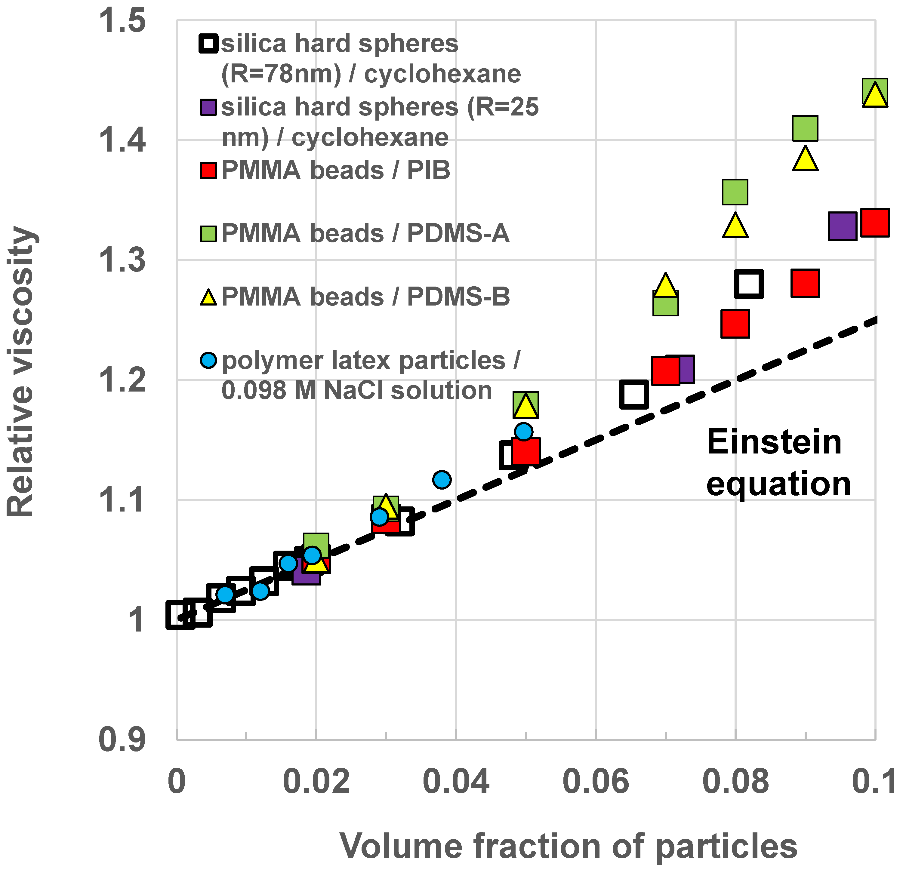
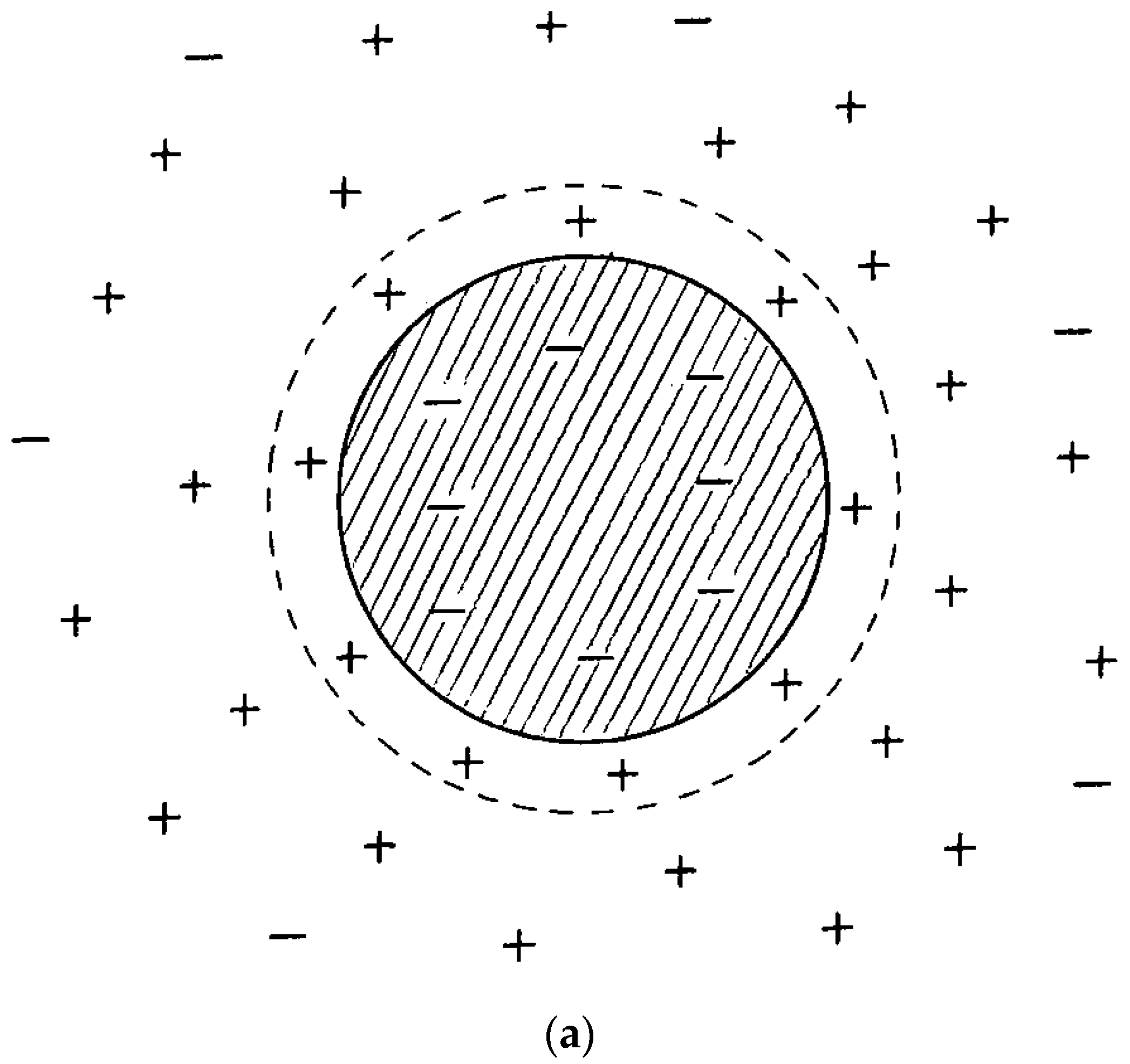
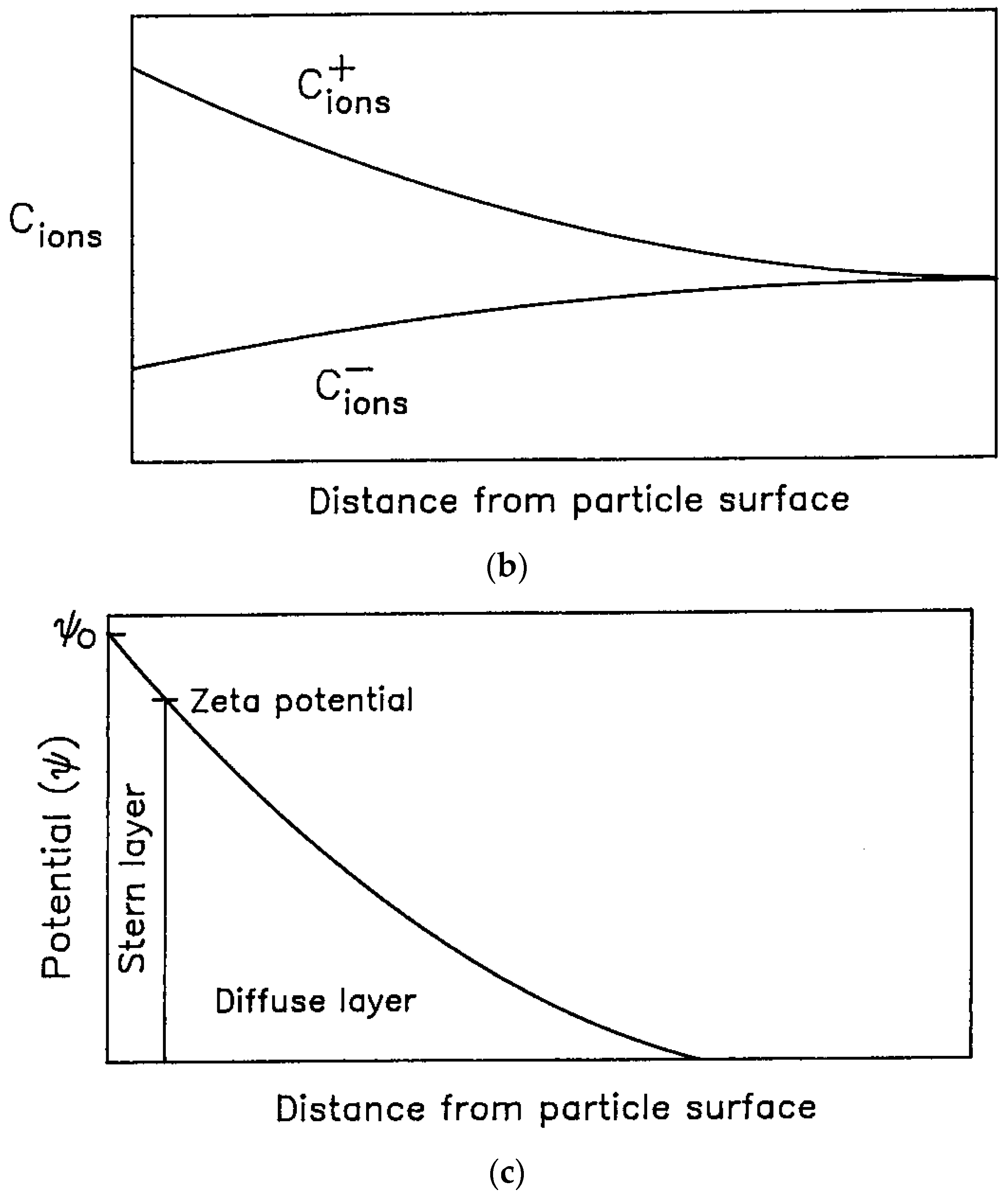
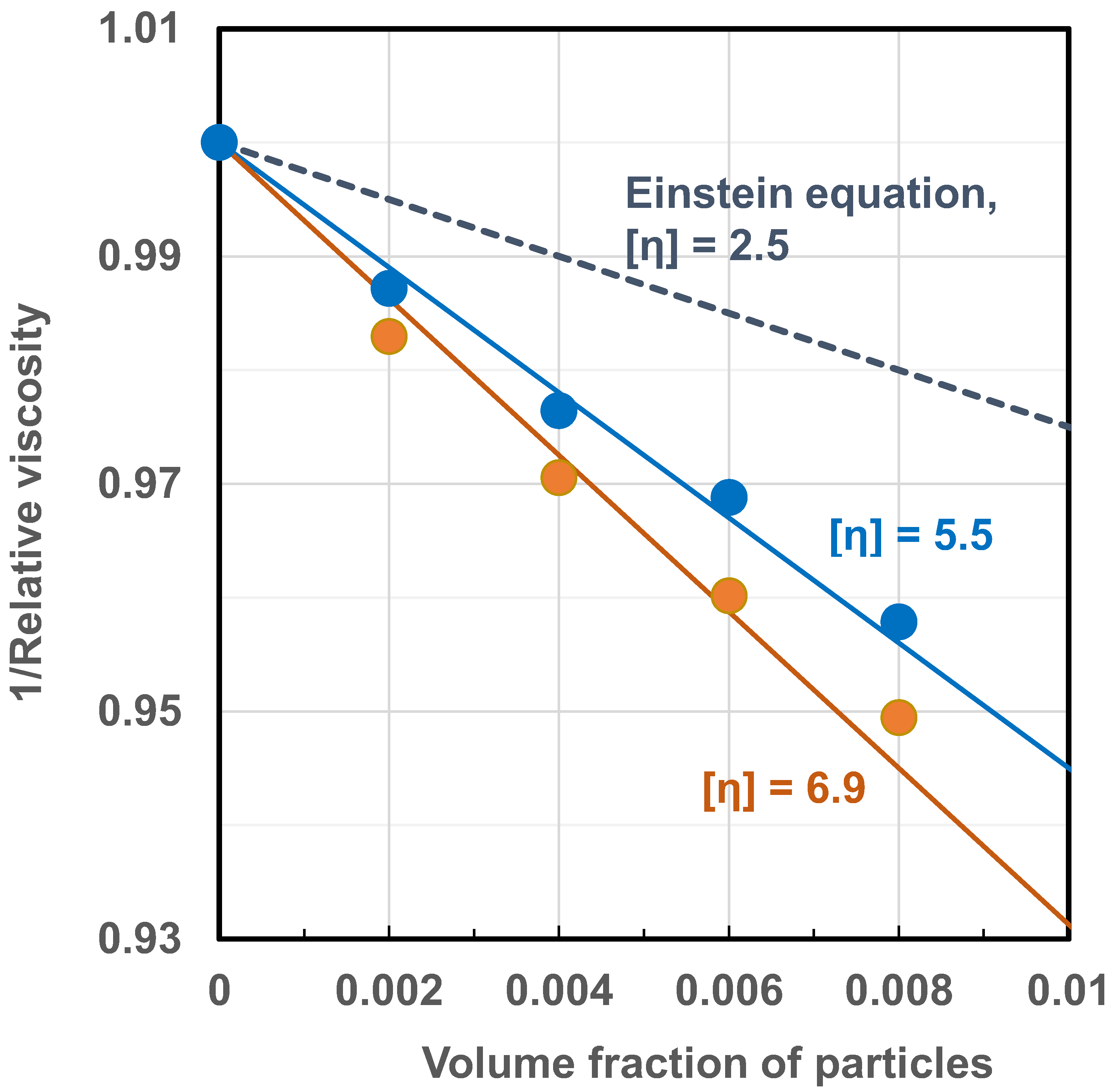

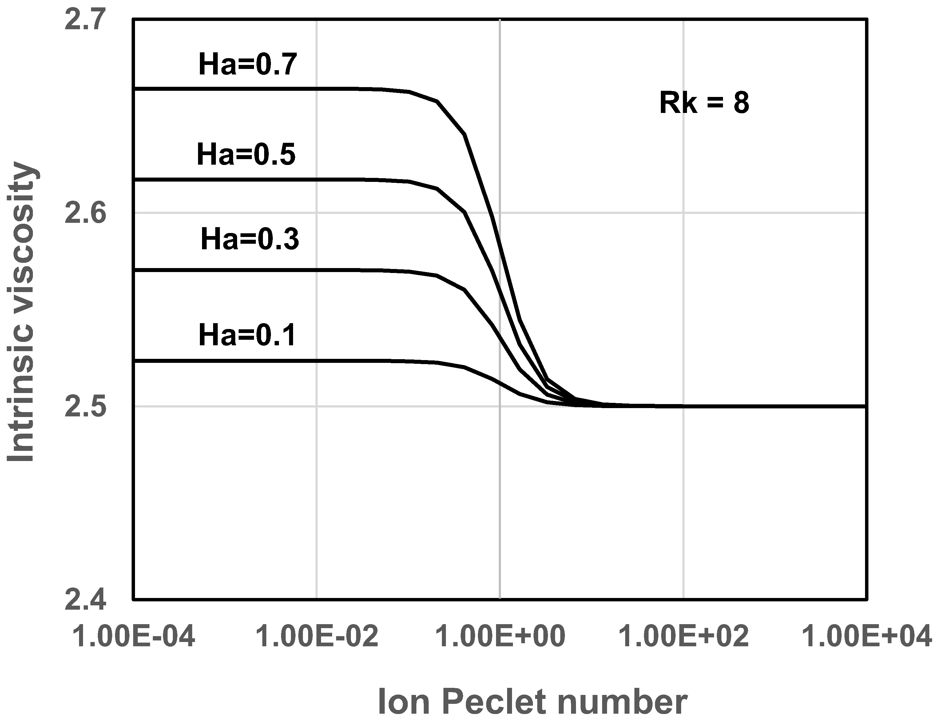
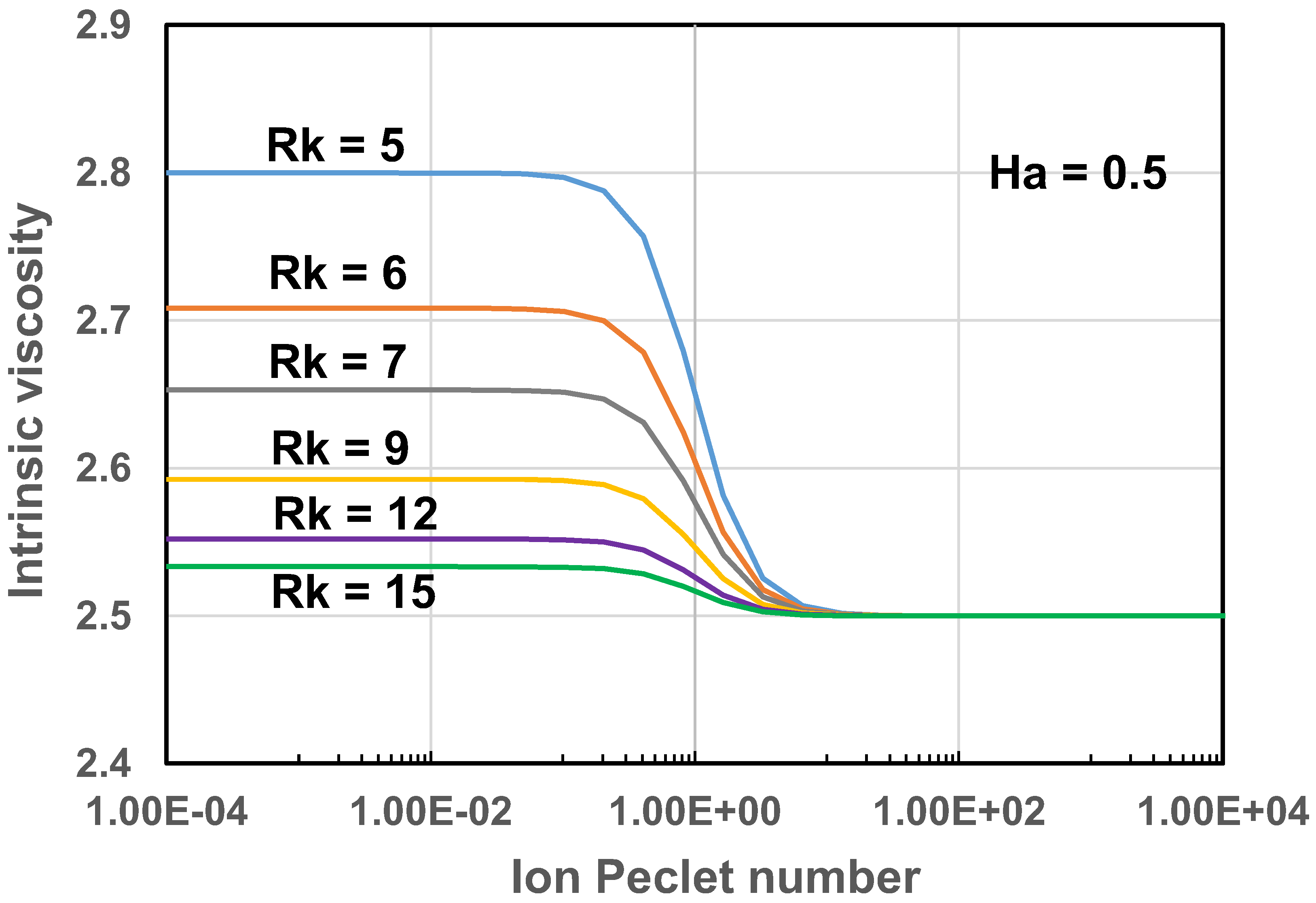
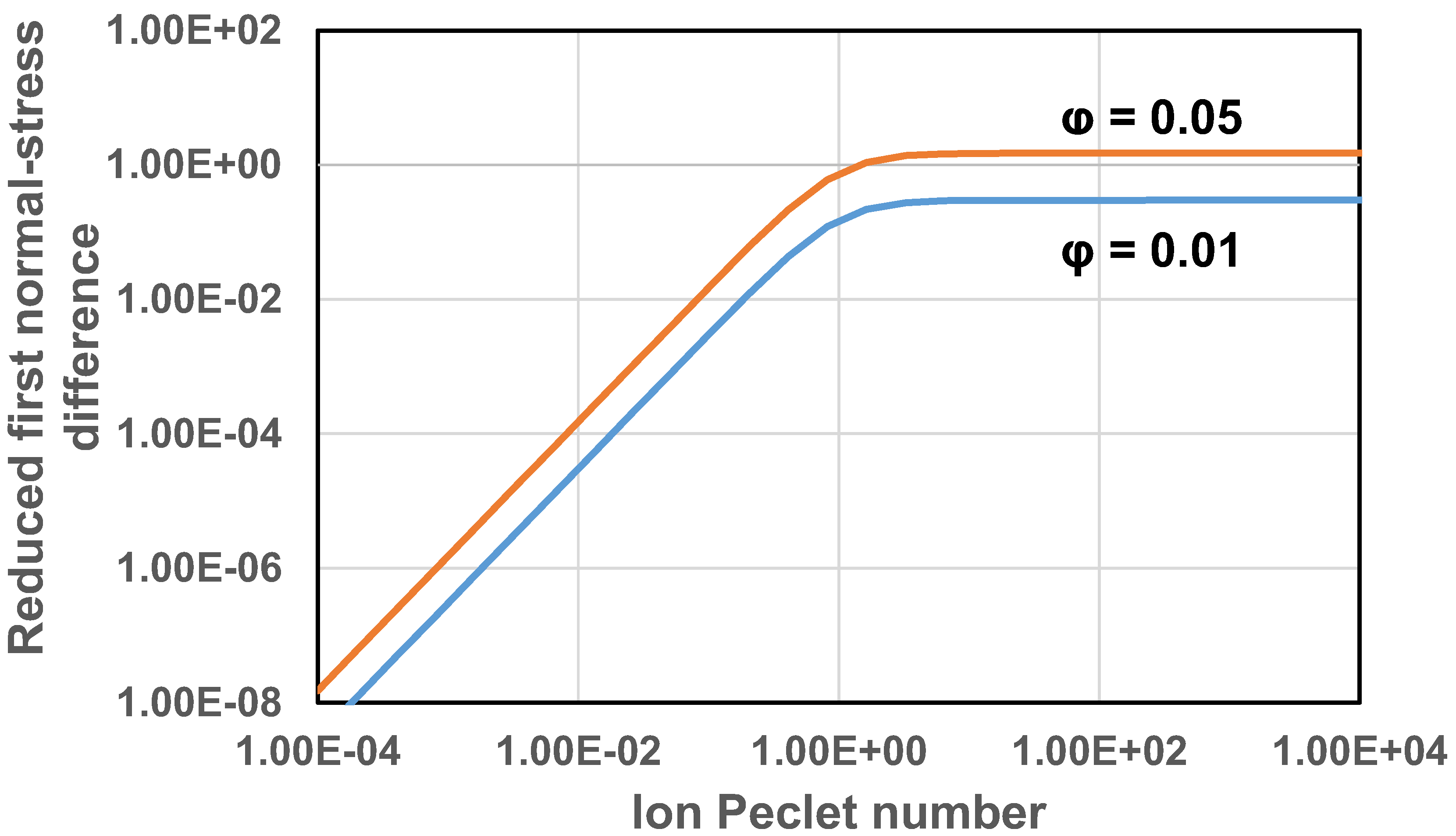
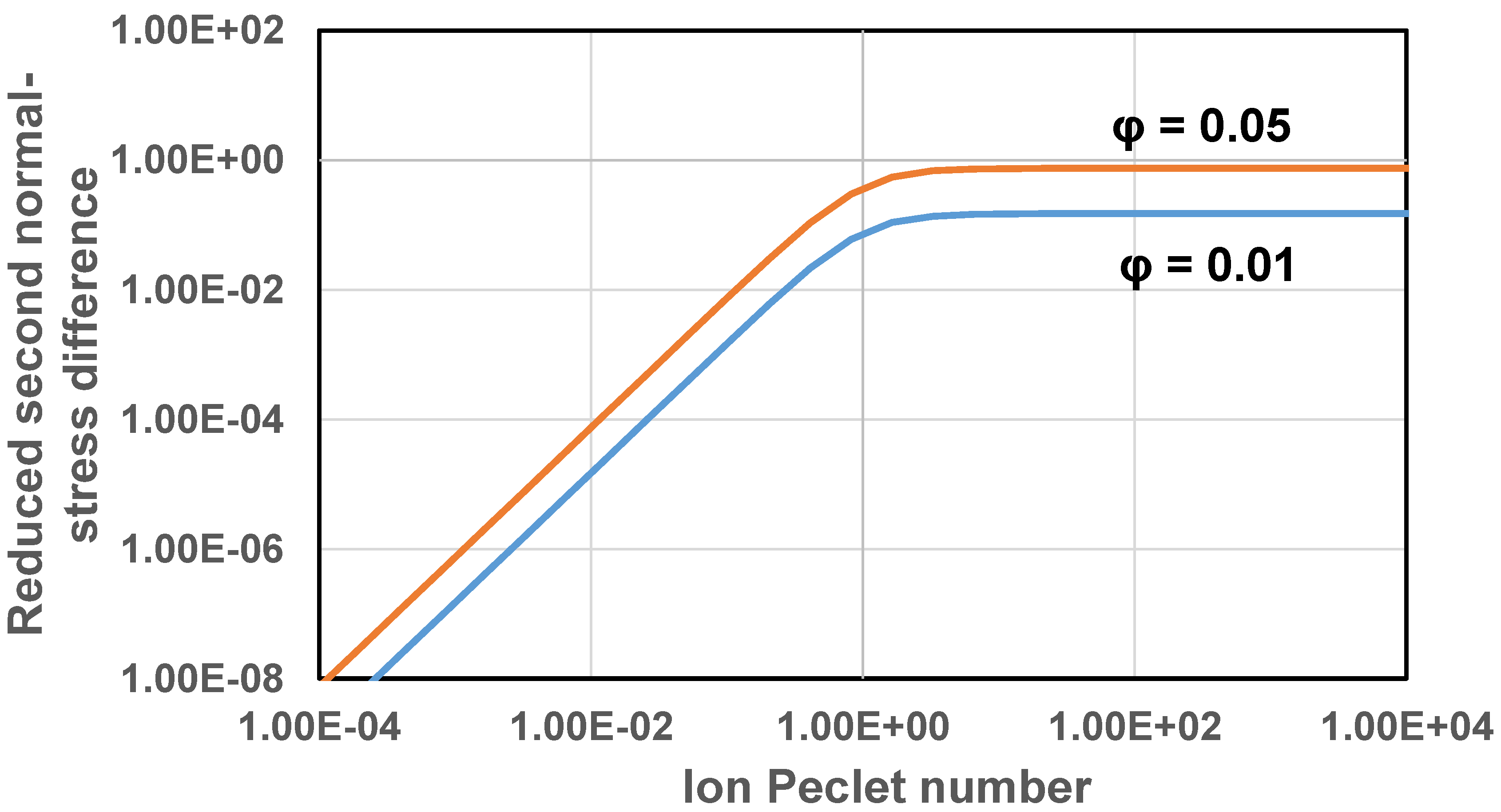


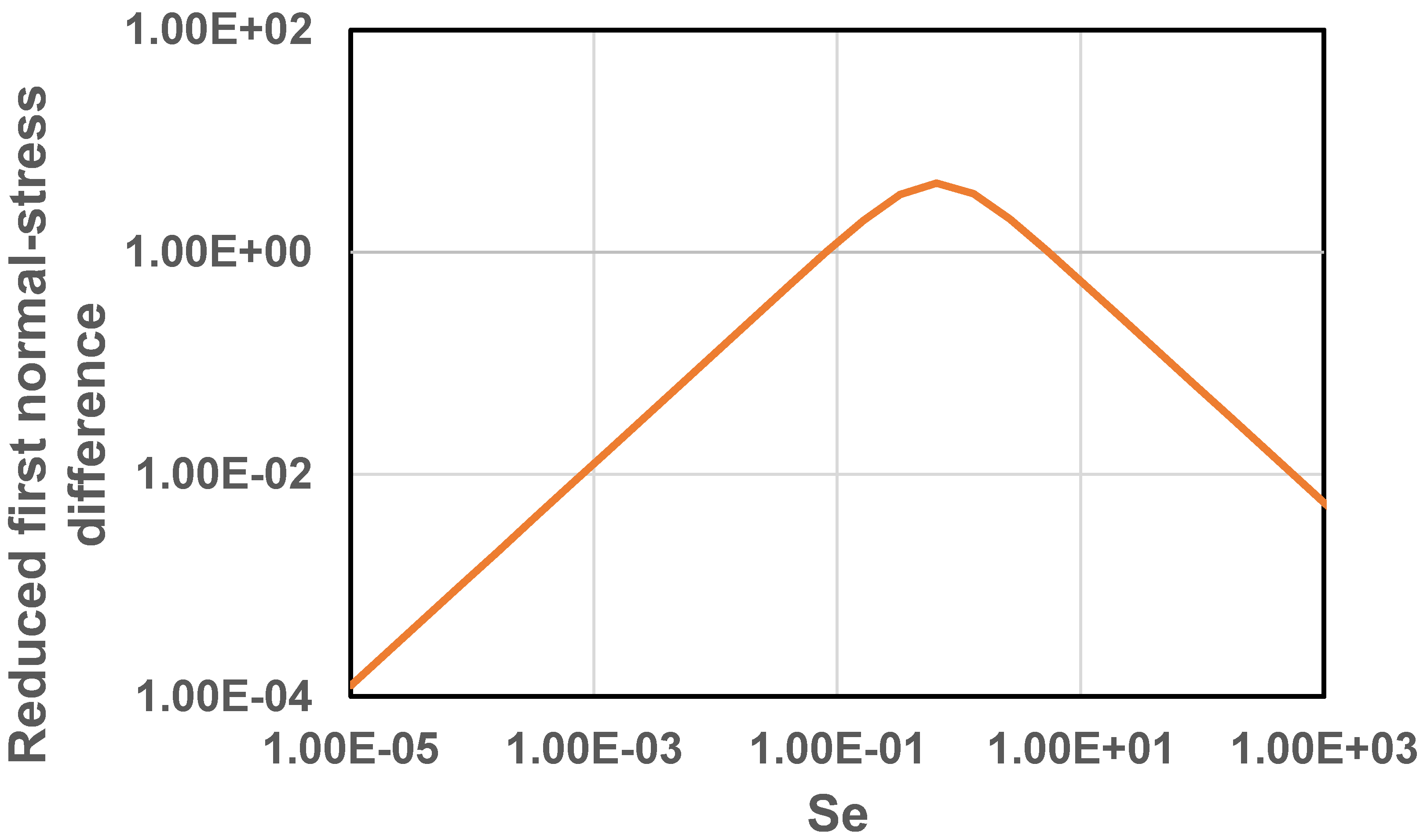
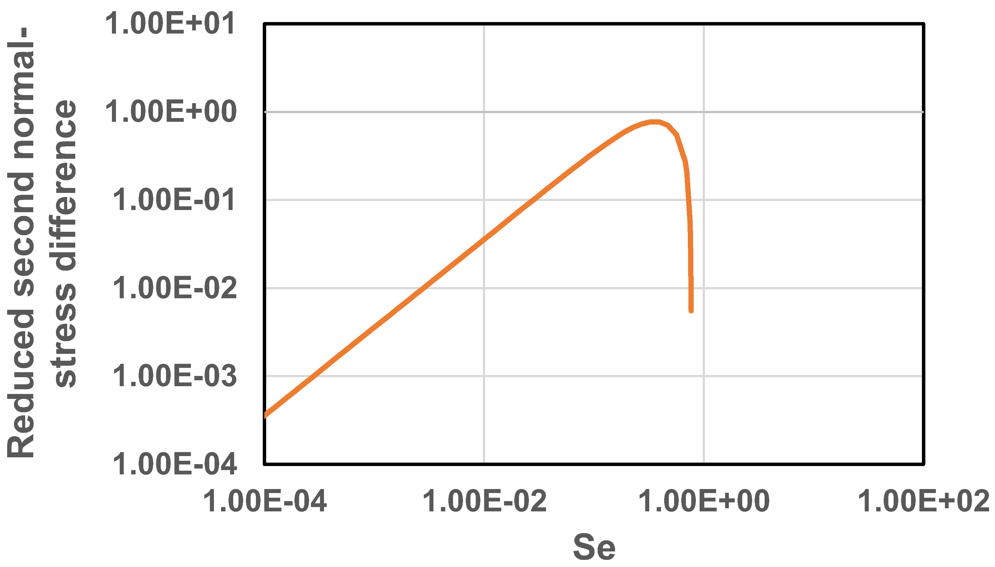

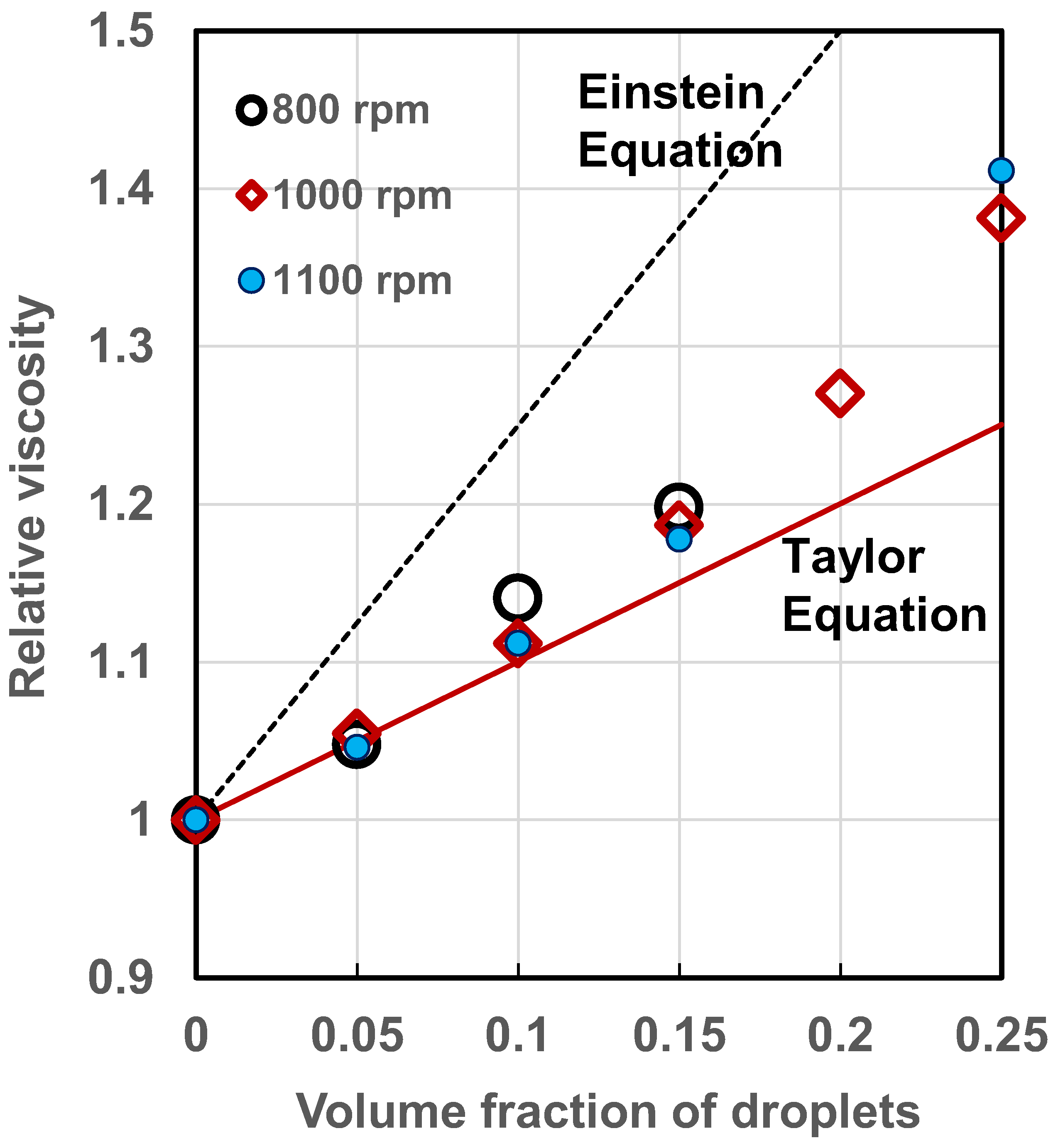
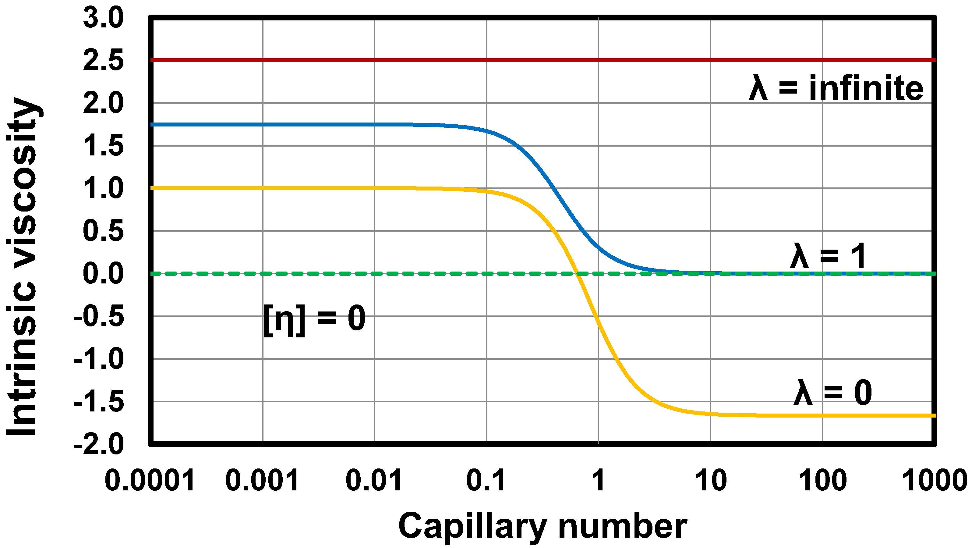
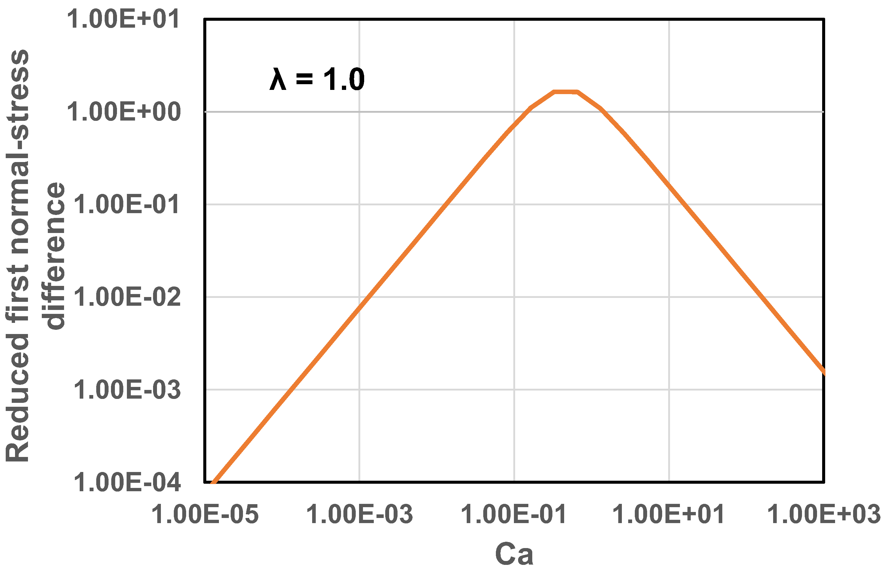

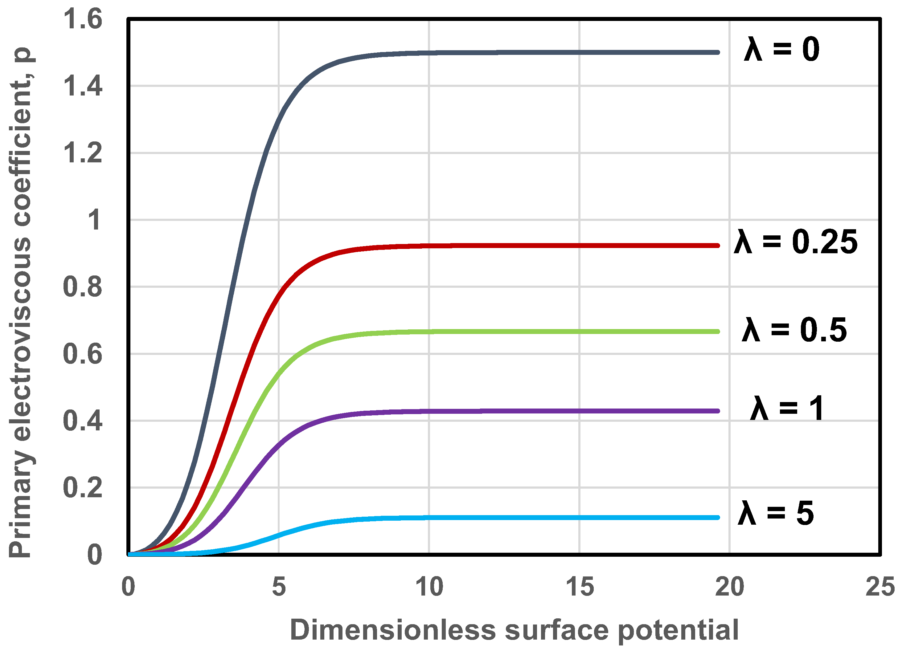

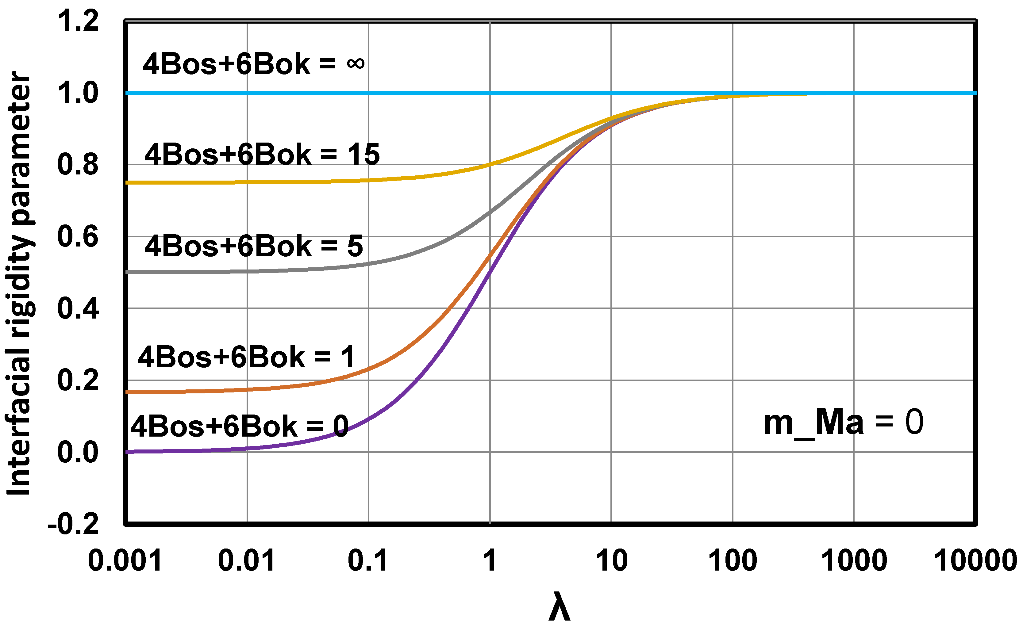
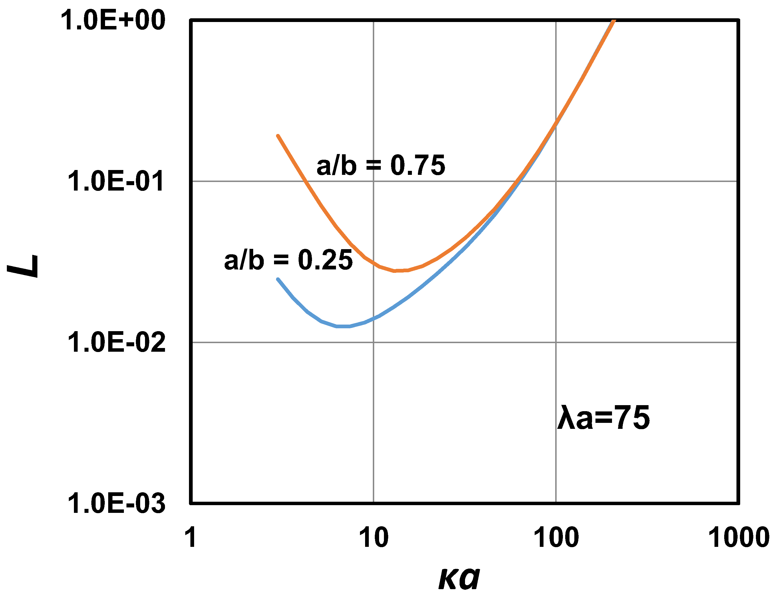
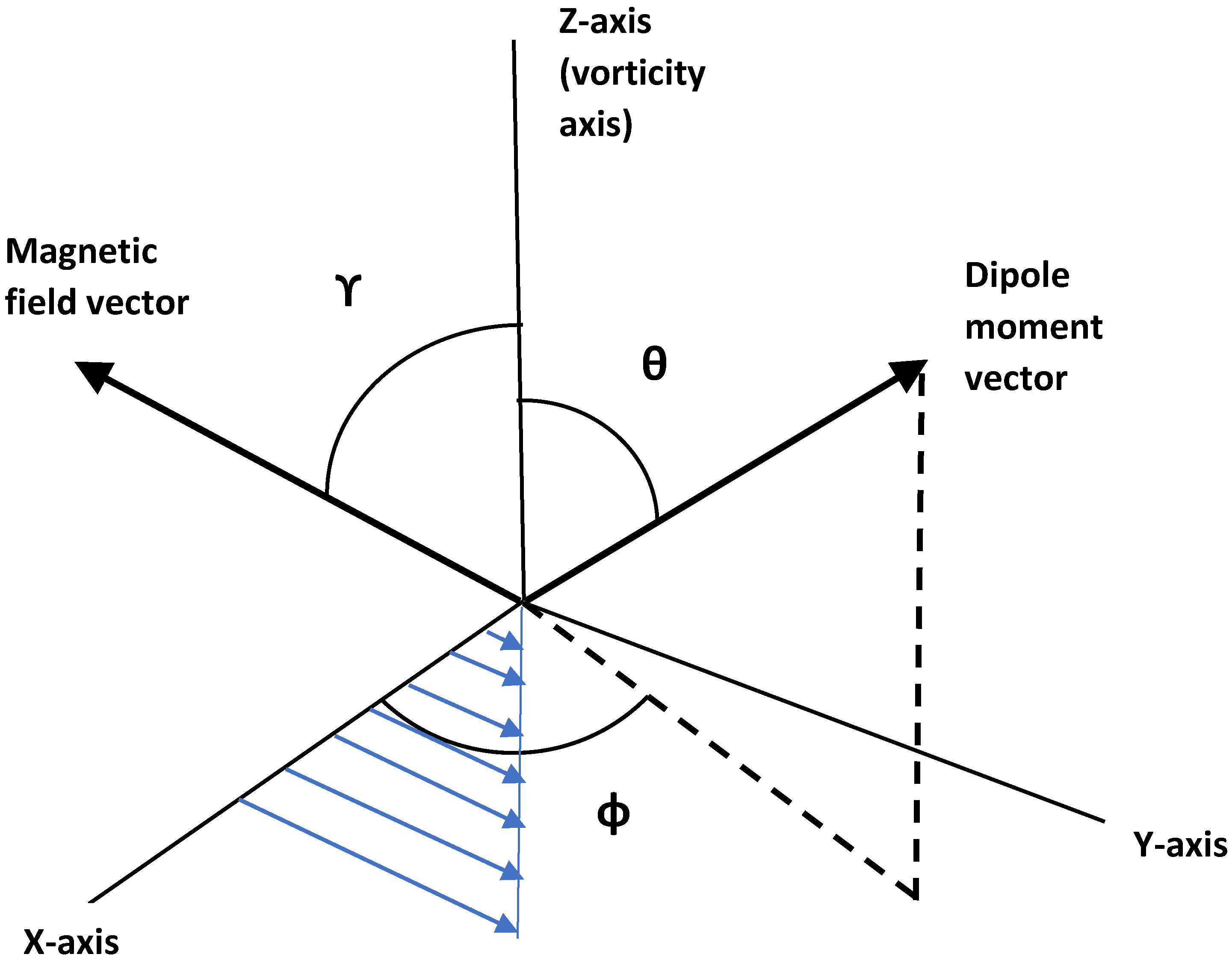
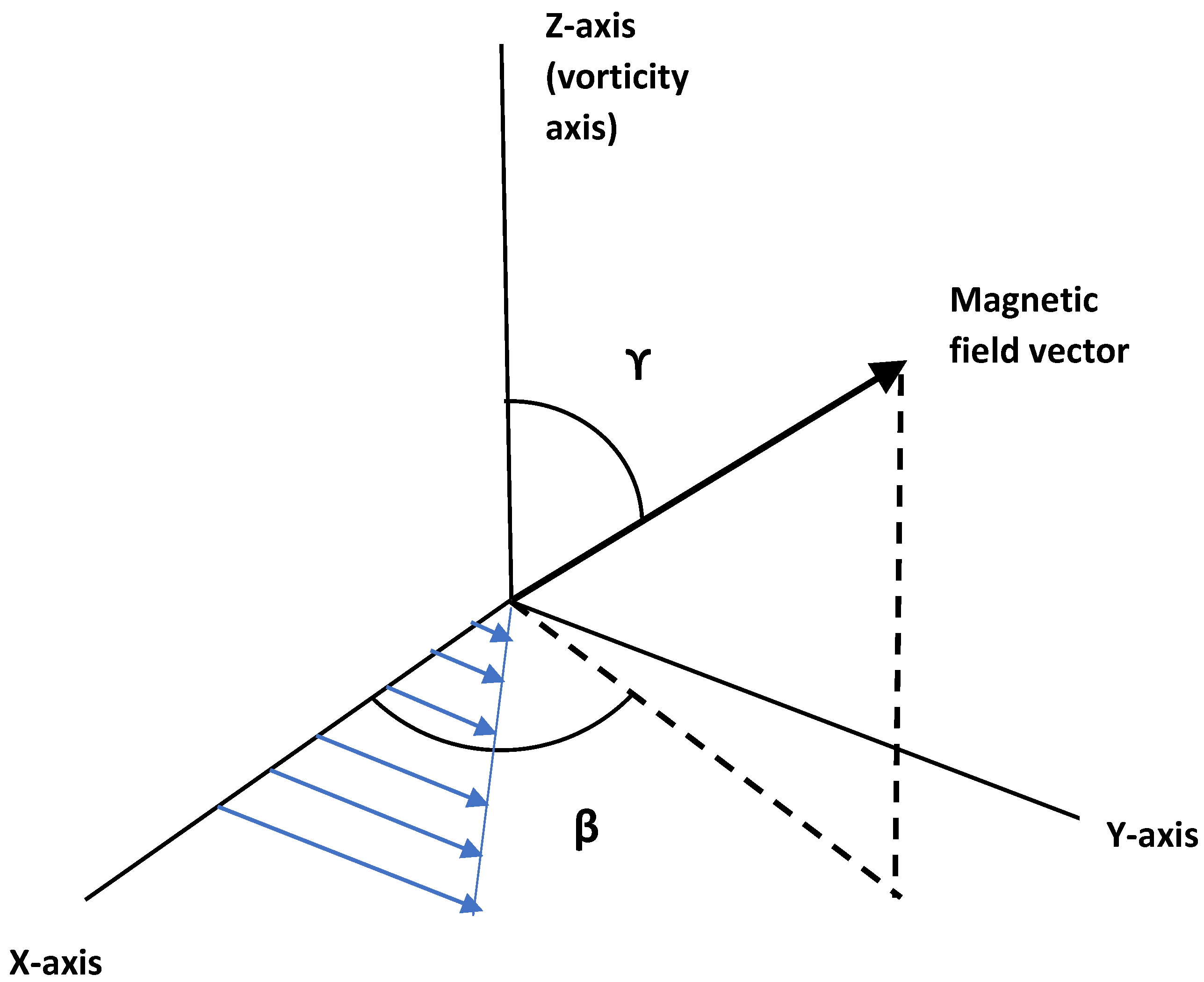
© 2016 by the authors; licensee MDPI, Basel, Switzerland. This article is an open access article distributed under the terms and conditions of the Creative Commons Attribution license ( http://creativecommons.org/licenses/by/4.0/).