Abstract
Shape memory polymers (SMPs) are soft active materials, their special property is the ability to hold a temporary shape and when exposed to a suitable trigger, they come back to their original shape. These external stimuli can be temperature, light or electro-magnetic fields. Amorphous SMPs are a class of thermally-activated SMPs that rely on glass transition to retain their temporary shape. Above the glass transition temperature (T > Tg), (amorphous SMPs exhibit finite deformation and viscoelastic behavior. In this work we develop a model to capture the viscoelastic behavior of the amorphous SMPs at elevated temperatures. The model uses an approach that was initially developed to study non-Newtonian viscoelastic fluids. We accomplish this by developing a multi-branch model based on the theory of multiple natural configurations using the maximization of the rate dissipation to determine the evolution of the natural configurations. We apply our model to study several different deformations at an elevated temperature T = 130 °C and show that this approach is able to capture the viscoelastic behavior of these polymers. The predictions of the theory are then compared with experimental results.
1. Introduction
Shape memory polymers (SMPs) are soft active materials that can be deformed and fixed in a temporary shape that remains stable, until exposure to an external stimulus which triggers the recovery to the permanent shape [1]. The external activating stimuli can be temperature [2,3], light [4,5], chemical environment [6], electromagnetic field [7,8], or specific solvent [9]. The latter two stimuli can be thought of as indirect thermally-triggered behavior. In literature, the first generation of SMPs was thermally-activated [1] and has been widely studied. Compared to shape memory alloys, SMPs possess many advantageous features, such as being inexpensive, easy to manufacture, and highly durable [10]. In addition, many SMPs can be made biocompatible and biodegradable by tuning them chemically [11]. Most significantly, SMPs have the ability to recover their shape even after undergoing large strains (to the order of 400%) [12]. Based on these advantages, SMPs are finding a wide range of applications in various fields, such as arterial stents in the biomedical field [13], as actuators and sensors in microelectromechanical systems (MEMS) [14,15], and in additive manufacturing [16,17], to name a few.
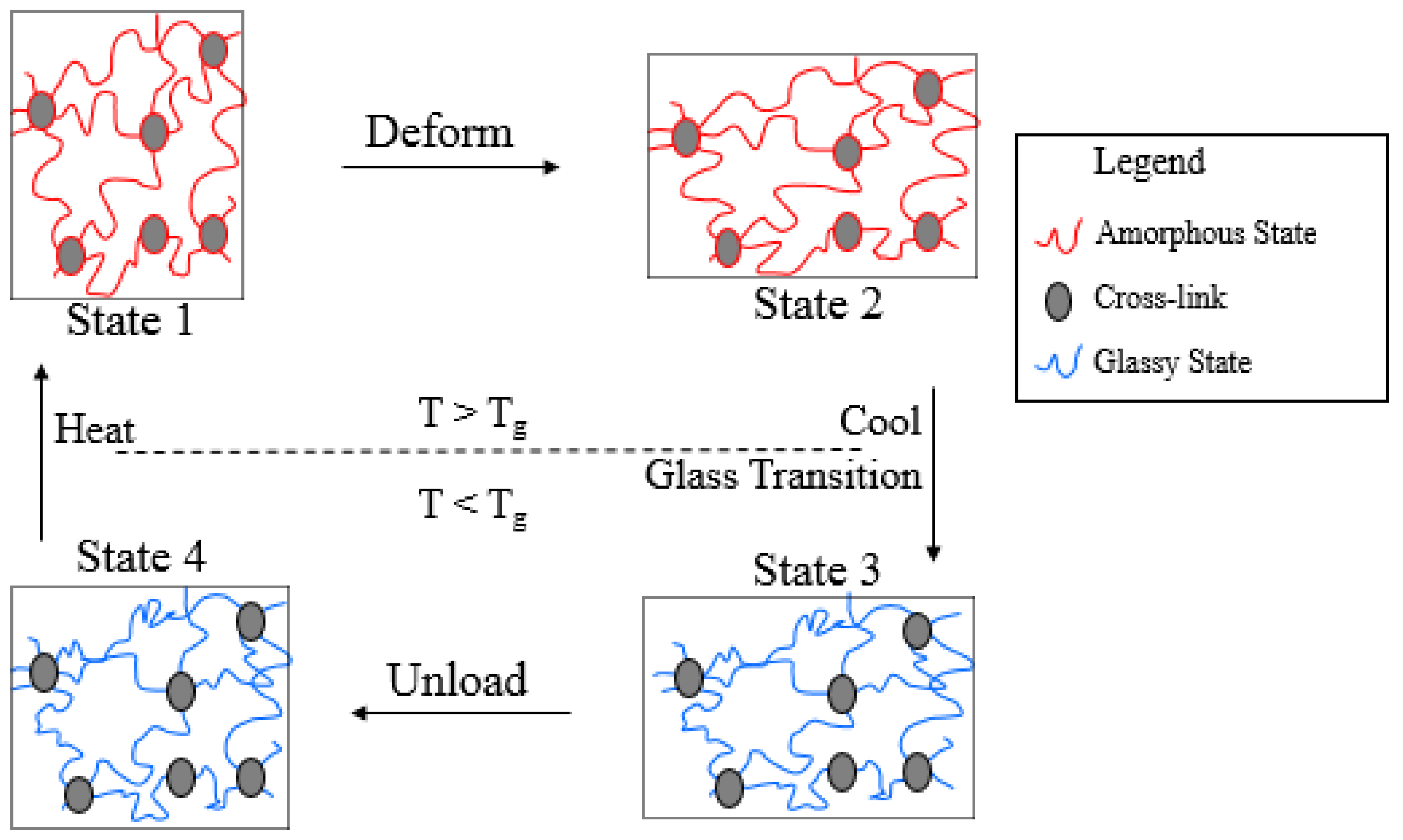
Amorphous SMPs are a type of SMPs which are thermally triggered, in which the shape fixation and the shape recovery effect is governed by glass transition. A typical shape memory cycle of amorphous SMPs is schematically illustrated by Figure 1. When the temperature is above the glass transition temperature (T > Tg), the undeformed polymer is in an amorphous state and exhibits viscoelastic behavior (State 1). Upon deformation, the material, and hence the polymer molecules, stretch (State 1 to State 2). If the polymer is now cooled below its glass transition temperature, the polymer molecules will lose their mobility due to glass transition and the modulus of the material increases dramatically (State 2 to State 3). If the material is now unloaded it will not revert back to its original shape but stays in a temporary shape (State 3 to State 4). This temporary shape is between the original shape and deformed shape due to the formation of the glassy phase in the deformed configuration. On heating above the glass transition temperature the original shape is recovered as the material regains its molecular mobility (State 4 to State 1). Based on the above description, it can be seen that in order to characterize the thermo-mechanical behavior of amorphous SMPs it is important to study their viscoelastic behavior at elevated temperatures (in State 1 to State 2). Furthermore, there are a number of polymers which behave in a manner similar to these polymers, and the model developed here can be applied to these types of polymers as well.
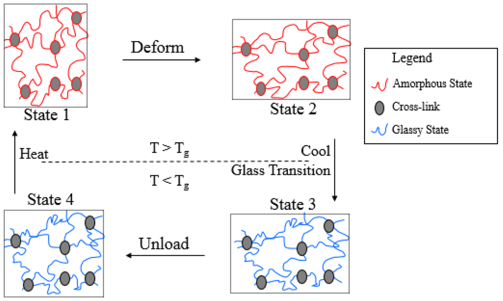
Figure 1.
Schematic illustration of shape memory cycle of amorphous SMPs.
Several different classes of amorphous SMPs have been reported recently, such as acrylate-based SMPs [13] and epoxy-based SMPs [18]. In this work, we study a class of epoxy-based amorphous SMPs (Veriflex-E) which have been characterized experimentally by McClung et al. [19,20]. Veriflex-E is commercially available and can be purchased from Cornerstone Research Group Inc. (CRG). The glass transition temperature (Tg) of the polymers is 98 °C obtained by a dynamic mechanical analysis (DMA) test. To capture the finite-deformation viscoelastic behavior of this polymer at an elevated temperature (T = 130 °C), we develop a multi-branch model. This model has two sets of branches: one equilibrium branch for the hyperelastic response and multiple non-equilibrium branches for the viscoelastic response. We use a Neo-Hookean model for the hyperelastic equilibrium branch, and the model of the viscoelastic non-equilibrium branch is developed using the theory of multiple natural configurations [21]. The material response of materials belonging to many different classes have been modeled using this framework, some of them are: multi-network polymers [22], metal plasticity [23], viscoelastic liquids [24,25], crystallization in polymers [26,27,28], crystallizable SMPs [29,30,31], and light-activated SMPs [32,33]. Classical elasticity and linear viscous fluids arise as simple cases within this theory. Though the problem we are tackling is isothermal, we develop the model in a thermodynamic setting. The amorphous polymer is modeled at elevated temperatures as a viscoelastic solid and the rate of dissipation is always positive. In this approach we have to choose forms for the Helmholtz potential and the rate of dissipation. These are then used in the reduced energy-dissipation equation, which is used to place restrictions on the forms for the stress. We further assume that the rate of dissipation is maximized, here it is associated with viscoelasticity. An identical approach has been used to model a number of materials in which entropy production takes place, for instance in twinning [21] and viscoelastic fluids [24]. We model amorphous Veriflex-E as a viscoelastic solid with two relaxation mechanisms. The model developed is used to solve problems of uniaxial tension, stress relaxation, and loading-relaxation-unloading cycles. The results are then compared against experiment data. The paper is arranged in the following order. Section 2 presents basic continuum theories used to derive our model. Section 3 introduces the finite deformation constitutive model. Section 4 presents the comparisons between the experimental results and the model predictions.
2. Preliminaries
Considering a body in reference configuration , let denote a typical position of a material point in and be the configuration of the body at time t. Then the motion assigns to each particle in configuration a position in the configuration at time t, and it is defined as:
We shall assume this motion and all the other quantities defined are sufficiently smooth to make all the operations meaningful and possible. The deformation gradient is defined as:
The left and right Cauchy-Green tensors are defined through:
Any acceptable process has to satisfy the appropriate conservation laws. The conservation equations appropriate for studying the viscoelastic behavior of glassy SMPs at elevated temperatures are the conservation of mass, linear and angular momentum, and energy. As the problem we are studying is an isothermal problem, the energy equation need not be considered. Furthermore, we assume that the material is incompressible. The conservation of mass for an incompressible material reduces to:
where v is the velocity. The conservation of linear momentum is:
where is the acceleration due to gravity, is the density, is the Eulerian velocity gradient and is sometimes denoted by and is the Cauchy stress tensor. For an incompressible material, the stress tensor reduces to:
where is the indeterminate part of the stress due to the constraint of incompressibility, and is the constitutively-determined extra stress. The balance of angular momentum for a body in absence of internal couples requires that the stress tensor be symmetric. In this work, we use the reduced energy-dissipation equation to place restrictions on the constitutive equations. The reduced energy-dissipation equation for an isothermal process is:
where is the Helmholtz potential, is rate of entropy production and is the rate of dissipation. Both and are constrained to be non-negative for an acceptable process.
3. Model Description
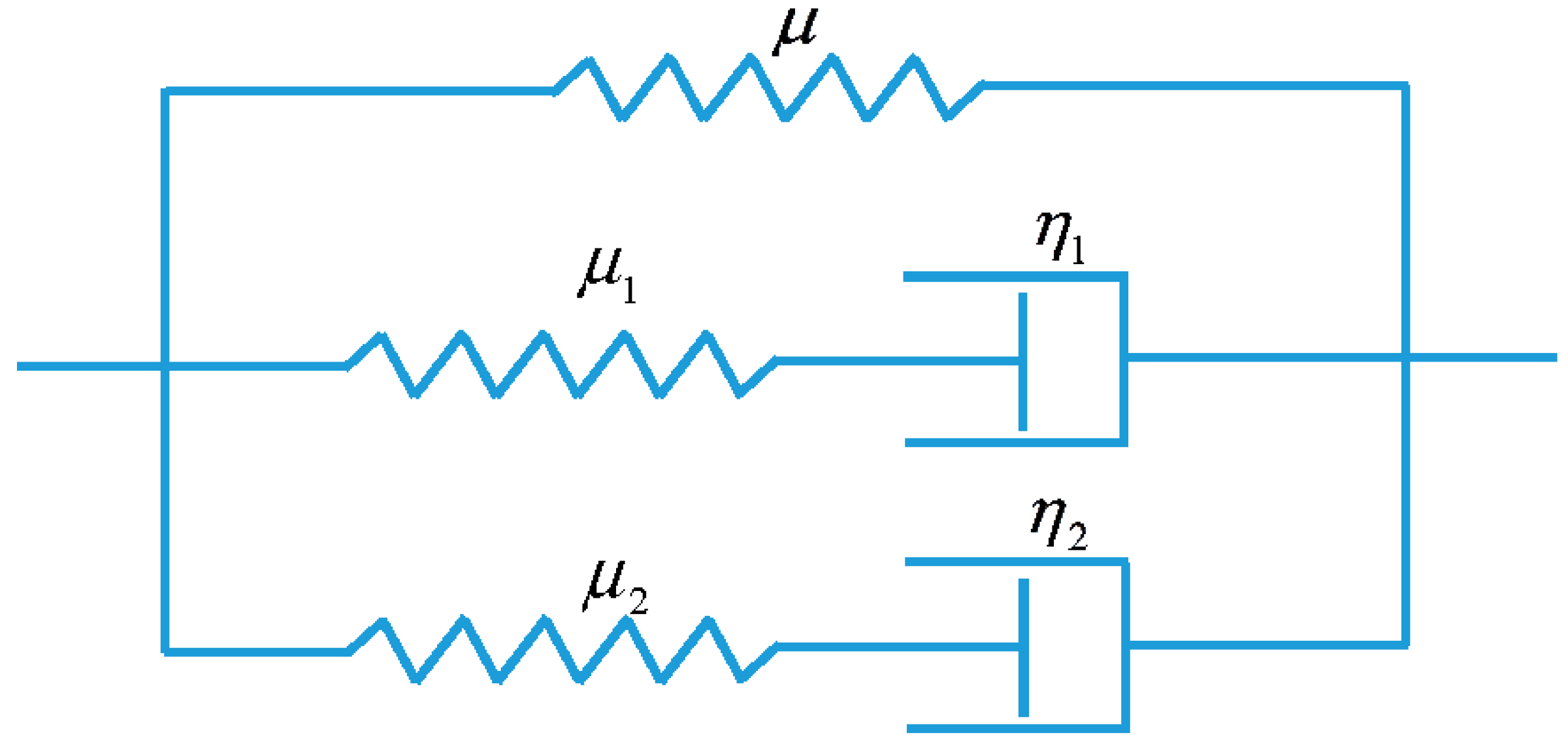
In order to model the viscoelastic behavior of the amorphous SMPs (Veriflex-E) at an elevated temperature (T = 130 °C), a multi-branch model for viscoelastic solids is developed. Here, we assume that the behavior of the polymer is characterized by two independent relaxation mechanisms but follows identical viscous flow rules. Thus, we require one equilibrium branch to represent the hyperelastic behavior of the material and two non-equilibrium branches to represent the viscoelastic modes of relaxation. The 1D rheological representation of the proposed model is presented by Figure 2.

Figure 2.
1D rheological representation of the proposed model.
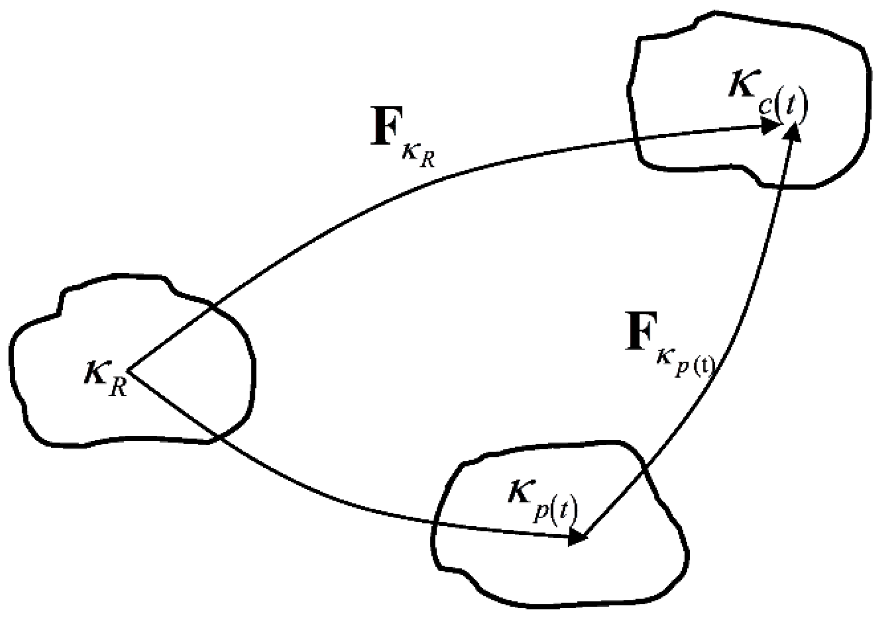
As mentioned above, we use the Neo-Hookean model to simulate the equilibrium hyperelastic behavior of the polymer. The derivation of the constitutive equations for the stress of non-equilibrium viscoelastic branch closely follows the work of Rajagopal and Srinivasa [24], which is based on the theory of evolving natural configurations. In this approach, the Helmholtz potential and the stress in the materials are determined from the mapping between the tangent spaces of the natural configuration at a material point to the current configuration occupied by it. In Figure 3, is a reference configuration, is the configuration currently occupied by the material and is the natural configuration associated with the material. The details of the theory and the derivation will be shown in Section 3.2.
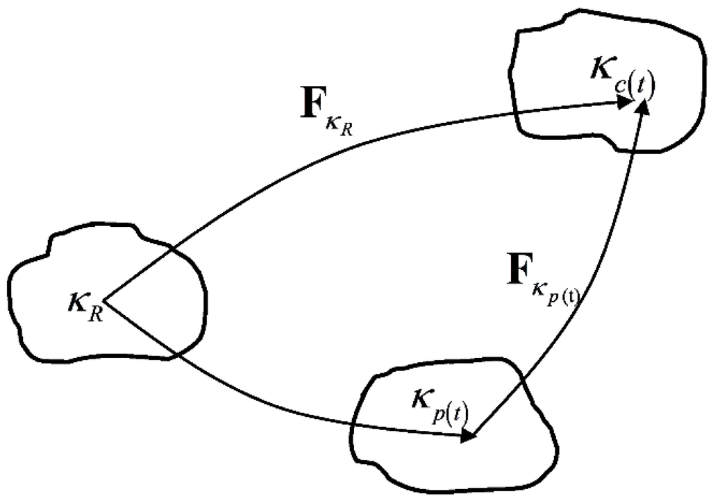
Figure 3.
Natural configurations associated with a single viscoelastic non-equilibrium branch.
A key feature of the material that has to be addressed relates to the incorporation of the thermal dependence into the model. In general we may require more than two non-equilibrium branches to simulate multiple relaxation mechanisms. The number of relaxation mechanisms of an amorphous SMP can be chosen to be equal to the number of Kuhn segments in a macromolecular chain, which can be evaluated from a limiting stretch experiment [34]. In this work, to simulate the viscoelastic behavior of the polymers at a specific elevated temperature, two non-equilibrium branches associated with the two relaxation mechanisms were sufficient. With sufficient experimental data, our model can be easily extended to a full thermo-mechanically coupled viscoelastic model by incorporating results from standard time-temperature supposition theories [35,36] as was done in Rao and Rajagopal [28]. In the following paragraphs, we will discuss the details of the models.
3.1. Hyperelsatic Behavior of the Equilibrium Branch
As discussed above, the incompressible Neo-Hookean model is used for the hyperelastic behavior of the polymers. The Cauchy stress tensor for the incompressible Neo-Hookean material is given by:
where is the shear modulus of the elastomer, is the Lagrange multiplier due to the incompressibility constraint and is the left Cauchy-Green tensor.
3.2. Viscoelastic Behavior of the Non-Equilibrium Branch
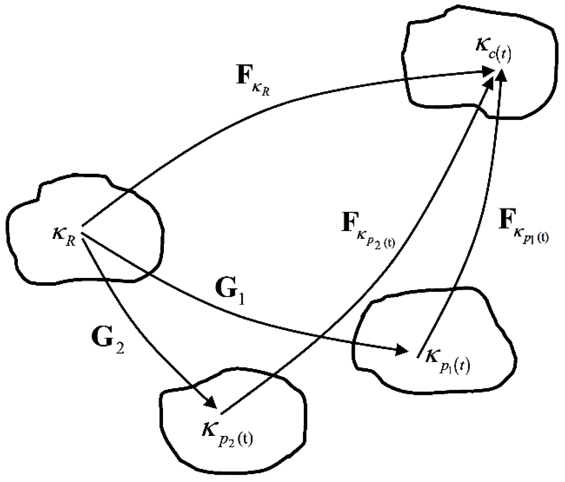
We have assumed that the material has two independent relaxation mechanisms associated with two non-equilibrium branches. In addition, we assume that the two relaxation mechanisms follow the same viscous flow rule. This is equivalent to the material possessing two independent natural configurations, each having the same evolution rule. The representation of the natural configurations of the material can be shown in Figure 4. and are the two natural configurations, is the original configuration and is the current configuration. Here we define and to be mapping between original configuration and the natural configurations and , respectively:

Figure 4.
Natural configurations associated with the polymer in the amorphous state having two relaxation mechanisms.
Further, we define the velocity gradient, , and the symmetric part of , to be:
In this approach, the left Cauchy stretch tensor plays the role of physically-motivated internal variables. It can be easily shown (for details see [26]) that:
where, the inverted triangle denotes the upper convected Oldroyd derivative and the dot is the material time derivative. Specification of is tantamount to prescribing the manner in which the underlying natural configurations change. As the material is incompressible, we shall assume that the motions associated with each of the natural configurations are isochoric:
We derive forms for , using the second law of thermodynamics in form of the reduced energy-dissipation equation and by requiring that the rate of dissipation be maximized. We make the following constitutive assumptions on the Helmholtz potential:
where is the Helmholtz potential of the amorphous phase. We further assume that the Helmholtz potentials associated with the two natural configurations are additive:
Since the amorphous state of the polymer is isotropic, the forms for and are those of an isotropic material and have the following forms:
where:
Since the material is isotropic, we can choose without any loss of generality, configurations and appropriately rotated such that:
where , are the right stretch tensors in the polar decomposition. We assume the following form for the rate of dissipation:
with the additional assumption that the rate of dissipation associated with a natural configuration is zero when it is not changing:
We also assume that the rate of dissipation associated with each natural configuration is non-negative:
Substituting Equations (12) and (16) into Equation (8) and using Equation (18), we get:
Since the second term of Equation (22) and the right-hand side are independent of D and nothing that only isochoric motions are permissible, it is sufficient to assume the stress has the form:
This assumption is sufficient to ensure that for all motions for which the natural configurations do not change, the material responds elastically. We also define the partial extra stresses associated with each of the natural configurations:
Using Equations (23) and (24), Equation (22) reduces to:
From the forms chosen for the Helmholtz potential and the rate of dissipation, it is clear that:
Equation (26) places restrictions on the tensors that are achievable. We assume that the actual value of chosen satisfies the constraints given by Equations (13) and (26) and also corresponds to a maximum for the rate of dissipation. This is enforced using the method of Lagrange multipliers by maximizing Equation (19) subject to the constraints given by Equations (13) and (26). On doing this, we obtain the following equations for the determination of :
where and are Lagrange multipliers.
For the problem under consideration, we assume that the Helmholtz potential associated with the elastic response of the amorphous phase is that of a Neo-Hookean material:
Additionally, we assume that the rate of dissipation has the form:
where the material constant is the elastic modulus and the material function is the viscosity of the material. With these assumptions, Equation (23) reduces to:
Equation (24) reduces to:
Substituting Equation (29) into Equation (27) and eliminating by using Equations (13) and (26), we obtain:
From Equations (12), (13), (18), (31) and (32) we obtain:
The relaxation times associated with the two natural configurations are given by:
This completes the development of the model for viscoelastic non-equilibrium branches.
3.3. Model Conclusion
Based on the above discussion, the total Cauchy Stress Tensor of the material is given by:
where the and are solved from Equation (33) with material parameters , and , respectively.
4. Applications
In this Section, we simulate the viscoelastic behavior of the material with the proposed model. We present the numerical procedure of how to solve the viscoelastic equations in Section 4.1. In Section 4.2, we discuss our approach of identifying the material parameters. Finally, in Section 4.3, based on the determined parameters we study the mechanical behavior of the material under uniaxial extension and loading-relaxation-unloading cycles at different strain rates.
4.1. Numerical Procedure
For uniaxial extension at a constant stretch rate, the stretch as a function of time is defined as:
where is the stretch rate and . For relaxation and unloading process, we use the same equation but have and , respectively. The velocity gradient then can be given as:
Substituting Equation (37) into Equation (33) and by prescribing the stretch rate we can facilitate ordinary differential equations (ODEs) for different viscoelastic deformations. To solve these ODEs, we require material parameters ( and ) and proper initial conditions. The identification of the material parameters will be discussed in Section 4.2. For the initial conditions, since the material is initially amorphous in a stress-free state, the following initial conditions for the tensors are given:
With respect to multistep simulations such as stress relaxations after uniaxial extension and loading-relaxation-unloading cycles, the final state of from the last step will be the initial condition of the next step. With material parameters and proper initial conditions, viscoelastic ODEs are solved to calculate the stress of the materials. In this work we use ODE45, which is a robust ODE solver provided by MATLAB, to solve the viscoelastic ODEs. The flowchart of the numerical procedure is shown in Figure 5.
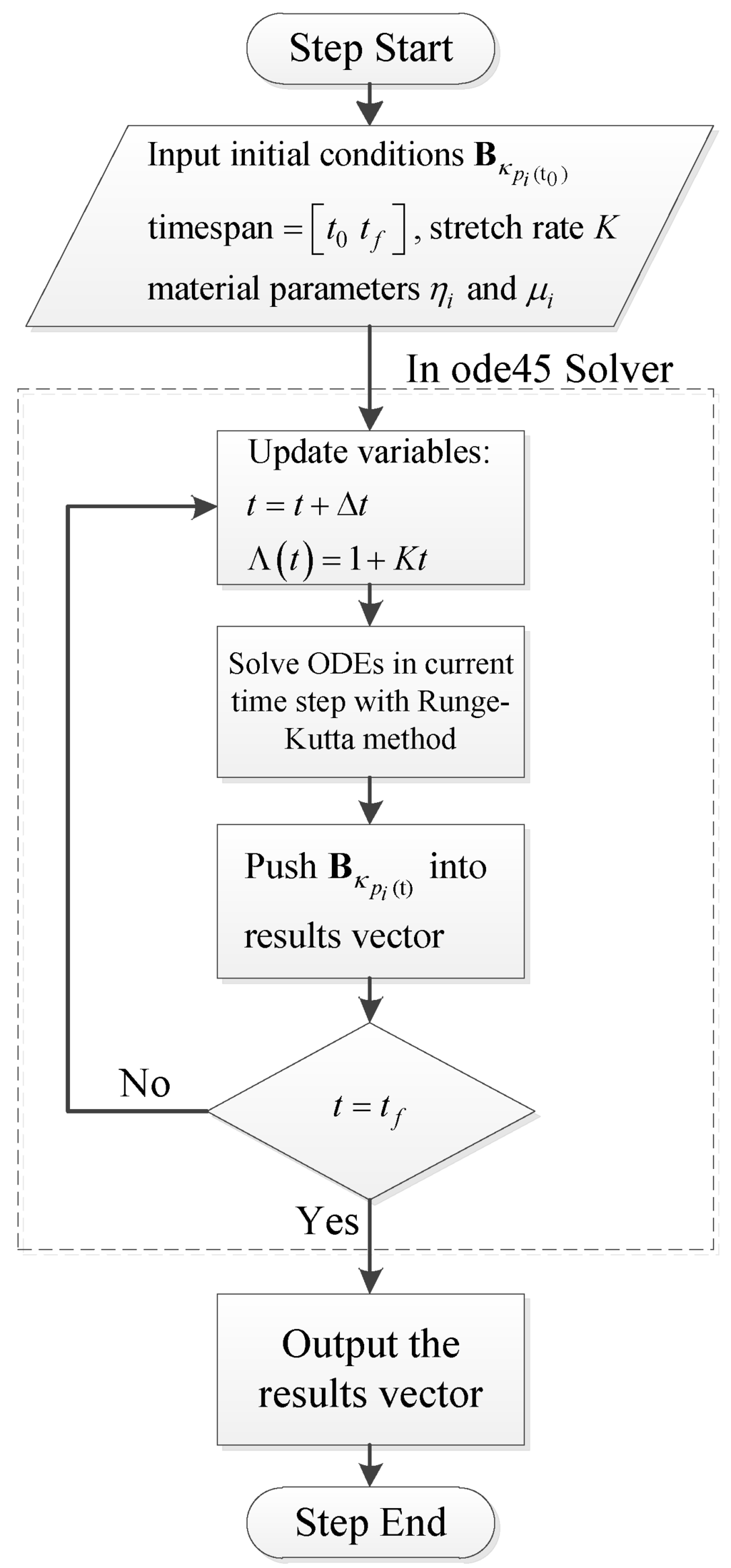
Figure 5.
Numerical procedure to solve viscoelastic ODEs.
Once the ODEs are solved the Cauchy stress of the materials can be calculated by Equation (35), and the Hencky strain (true strain) can be obtained through Equation (36).
4.2. Parameter Identification
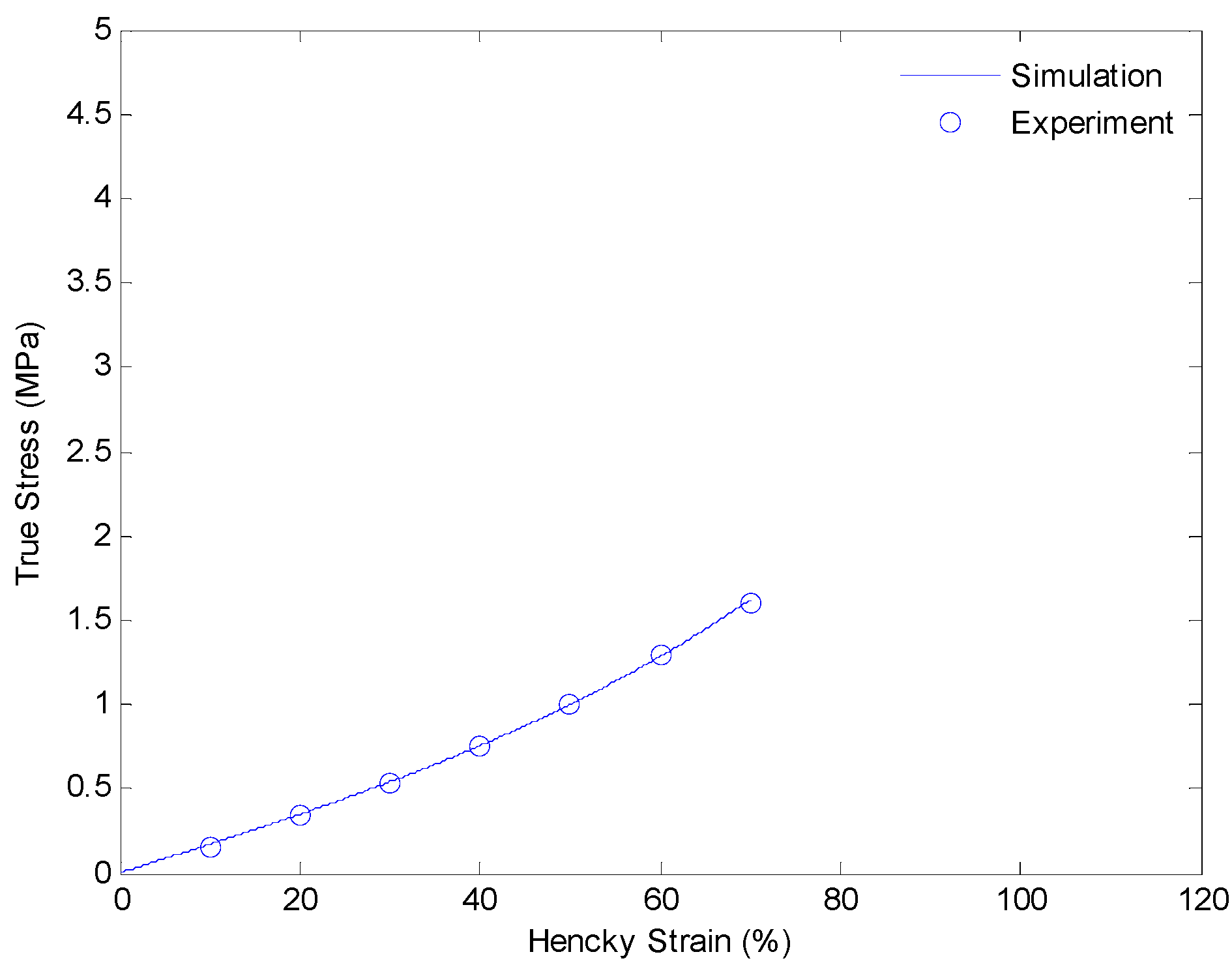
In this section, we discuss details of our strategy of identifying material parameters. We will determine the shear modulus of the equilibrium hyperelastic branch first. The shear modulus of the equilibrium branch is evaluated from experimental data of a uniaxial extension test with a strain rate of 0.0001/s. Since the deformation rate is very slow, and the relaxing speeds of non-equilibrium branches are relative faster, we assume the load is mainly taken by the equilibrium branch itself. Thus, the shear modulus can be evaluated by curve fitting the experimental data with Equation (9). The result is shown in Figure 6.
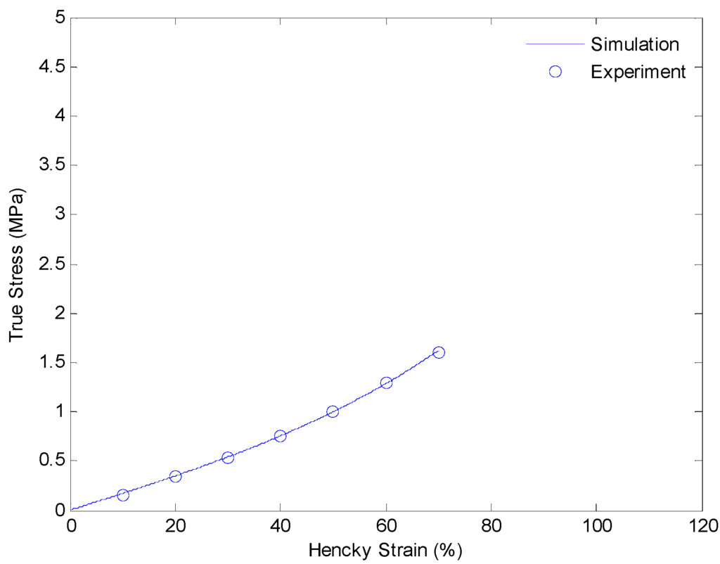
Figure 6.
Plot of true stress versus Hencky strain for uniaxial extension of SMPs at 130 °C with a strain rate of 0.0001/s.
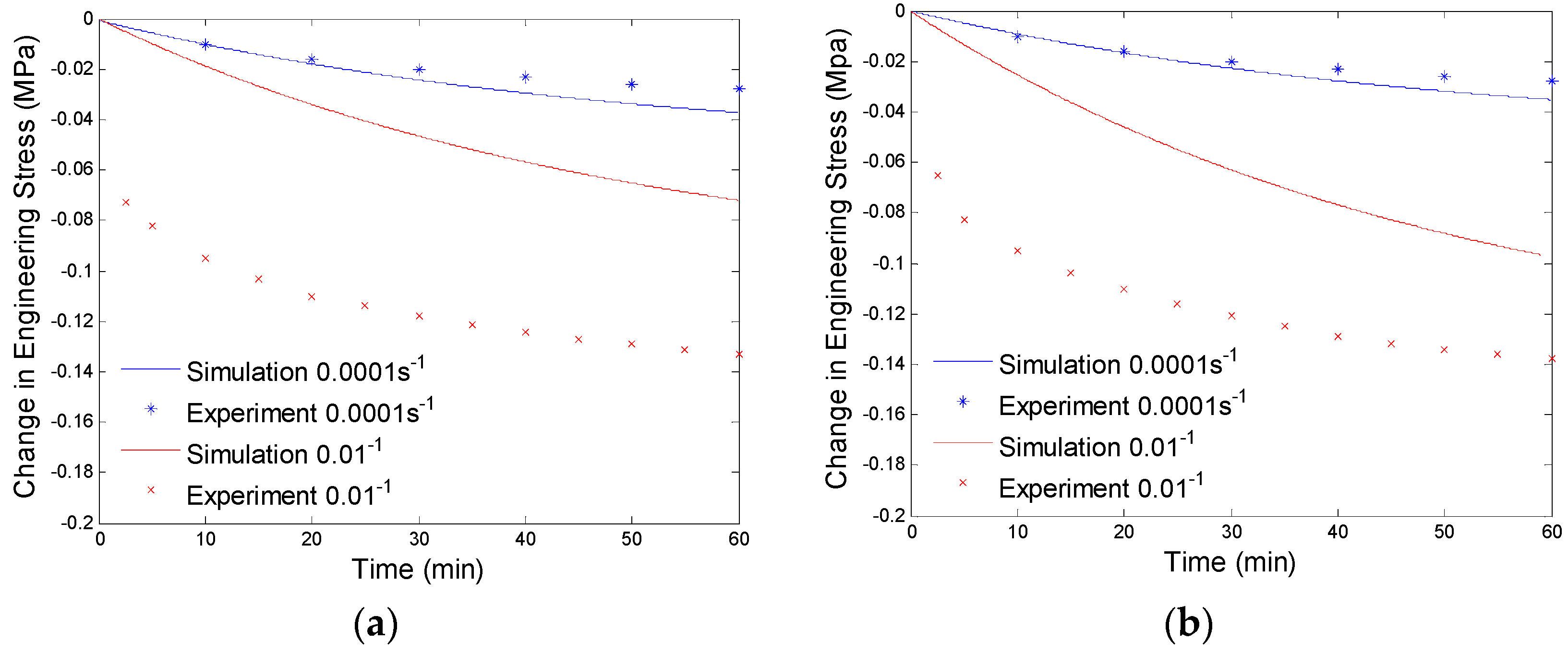
After getting the shear modulus of the equilibrium branch, we evaluate the shear moduli and viscosities of the non-equilibrium branches by using the experimental data from the stress relaxation tests under different preloading rates. Here, we assume two non-equilibrium branches have different relaxation times. One has a very small relaxation time and can only take loads under high strain rate loadings (0.01/s), the other has a relative large relaxation time and will take loads under both high rate (0.01/s) and low rate (0.0001/s) deformations. Here, we suppress the non-equilibrium branch with small relaxation time first and evaluate the modulus and viscosity of the non-equilibrium branch with large relaxation time through fitting the experimental data of stress relaxation at low preloading rate (0.0001/s). The amount of the stress relaxation is decided by the shear modulus of the branch, and the viscosity affects how fast the stress will be relaxed. We will use the numerical procedure discussed in Section 4.1 to curve fit the experimental data. The fitting results are shown in Figure 7.
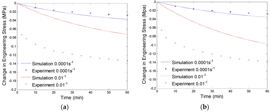
Figure 7.
Plot of change in engineering stress versus time for stress relaxation after a constant rate extension at 130 °C: (a) relaxation at 40% engineering strain; and (b) stress relaxation at 60% engineering strain. The simulation results are calculated with the equilibrium branch and one non-equilibrium branch.
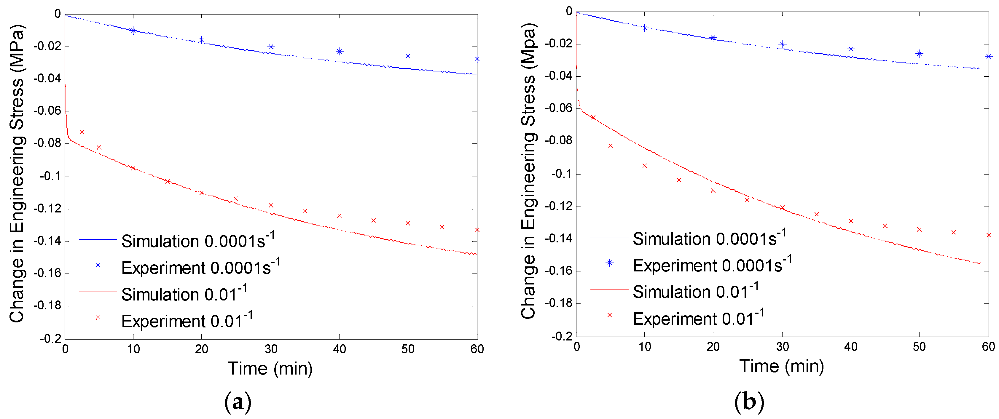
Since the parameters of the branch with a large relaxation time are evaluated by low preloading rate (0.0001/s) experimental data, the simulation results will not exactly fit the high preloading rate (0.01/s) experimental data (See Figure 7). Now we will determine the parameters of the branch with a small relaxation time by compensating for the high preloading rate (0.01/s) experimental data. This high relaxation time branch will not respond to low rate loadings, thus, it will not have any effects on the fitted experimental data at the preloading rate of 0.0001/s. By using the numerical procedure discussed in Section 4.1 and considering both the non-equilibrium branches, we get the curve fitting results shown in Figure 8. The material parameters of our model are shown in Table 1.
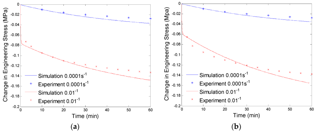
Figure 8.
Plot of change in engineering stress versus time for stress relaxation after a constant rate extension at 130 °C: (a) relaxation at 40% engineering strain; and (b) stress relaxation at 60% engineering strain. The simulation results are calculated with the equilibrium branch and two non-equilibrium branches.

Table 1.
Model parameters.
4.3. Results and Discussion
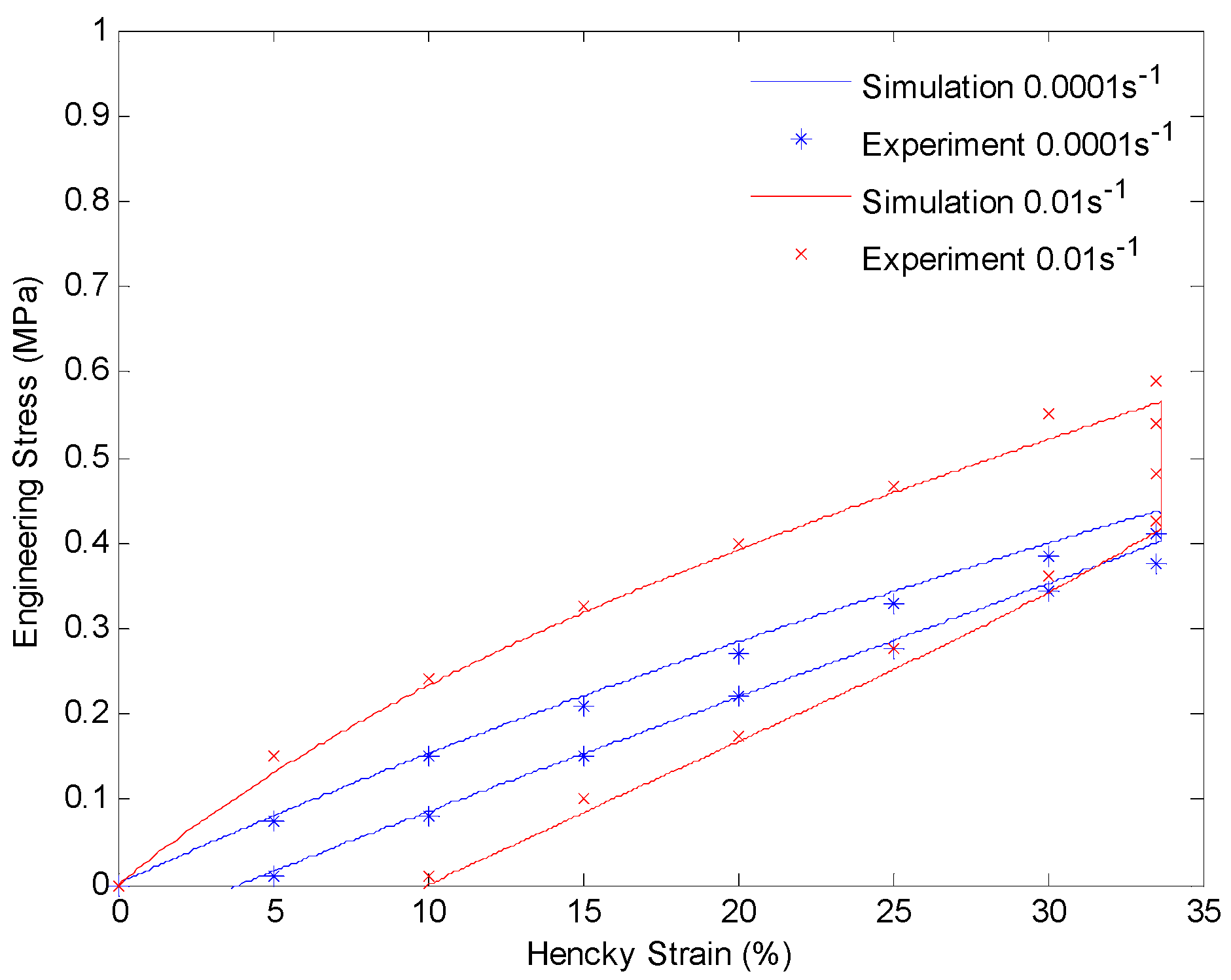
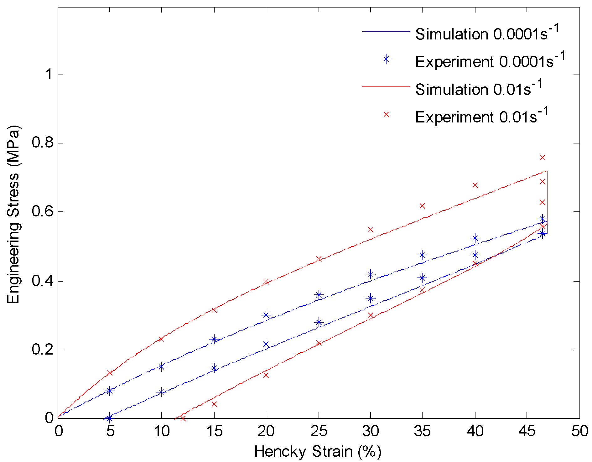
After getting all of the material parameters, we implement our model to simulate the uniaxial extension subjected to higher strain rates (0.001/s and 0.01/s) and loading-relaxation-unloading cycles. Figure 9 and Figure 10 show the simulation results of uniaxial tension at higher stretch rates of 0.001/s and 0.01/s, respectively. Figure 11 and Figure 12 show strain-stress curves of the loading-relaxation-unloading cycles. The data clearly shows that, at higher strain rates, the stress in the polymer is higher (Figure 9 and Figure 10), and for the polymer deformed at a higher strain rate, the stress relaxation is larger (Figure 11 and Figure 12). Additionally, at higher strain rates the strain at zero stress at the end of a loading-relaxation-unloading cycle is larger (Figure 11 and Figure 12). All of the results of the models are able to capture this behavior and match the experiment data well.
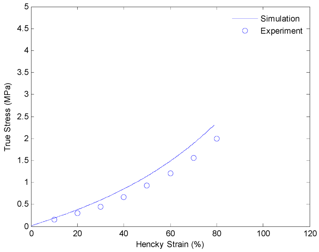
Figure 9.
Plot of true stress versus Hencky strain for uniaxial extension of SMPs at 130 °C with a strain rate of 0.001/s.
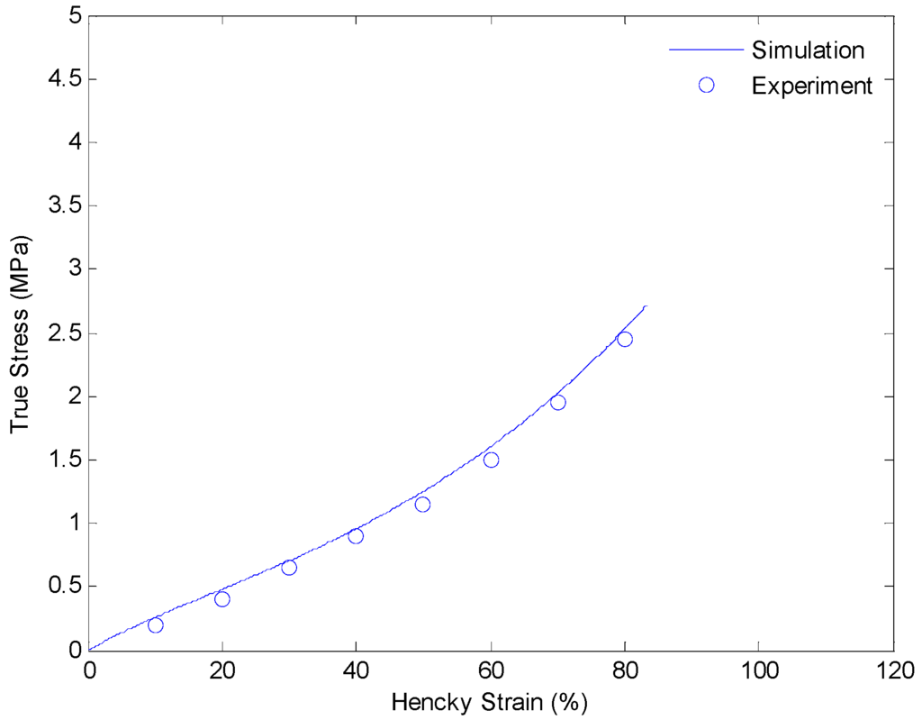
Figure 10.
Plot of true stress versus Hencky strain for uniaxial extension of SMPs at 130 °C with a strain rate of 0.01/s.

Figure 11.
Plot of engineering stress versus Hencky strain in a loading-relaxation-unloading cycle at 130 °C. The material is stretched to 40% engineering strain with a constant strain rate and held for 60 min. After that the material is unloaded with the same strain rate.
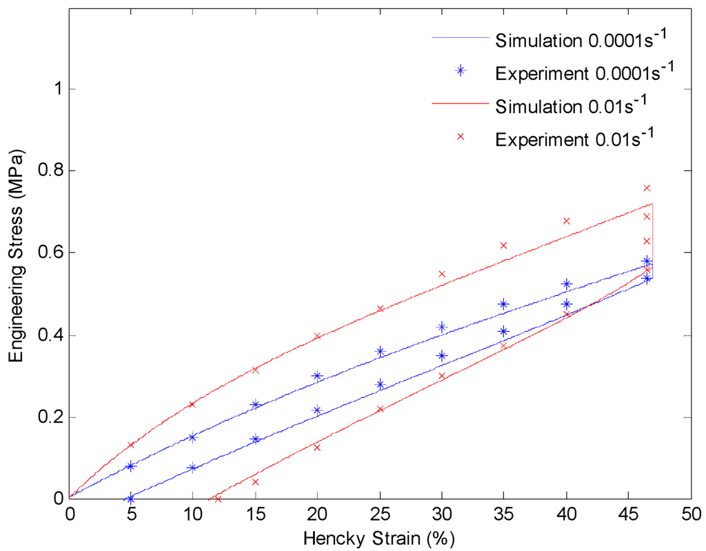
Figure 12.
Plot of engineering stress versus Hencky strain in a loading-relaxation-unloading cycle at 130 °C. The material is stretched to 60% engineering strain with a constant strain rate and held for 60 min. After that the material is unloaded with the same strain rate.
5. Conclusions
In this work, we have developed a multi-branch model to capture the viscoelastic behavior of a class of amorphous SMPs at an elevated temperature (above glass transition). The model is developed within a framework based on the theory of multiple natural configurations and the maximization of the rate of dissipation to determine the evolution of the natural configurations. The derivation uses the approach developed by Rajagopal and Srinivasa [15] for non-Newtonian fluids. The model is applied to simulate the polymer undergoing different deformations. The results of the model are compared against experimental data collected for a commercially available amorphous SMP, Veriflex-E. The simulation results match the experimental data well. This work opens the door for future studies of amorphous SMPs.
Acknowledgments
The authors would like to acknowledge the National Science Foundation, Grant #0900278 for partially supporting this work.
Author Contributions
Fangda Cui and I. Joga Rao designed the constitutive model and conducted the study. Fangda Cui and Swapnil Moon performed the numerical calculations and data analysis.
Conflicts of Interest
The authors declare no conflict of interest.
References
- Lendlein, A.; Kelch, S. Shape-memory polymers. Angew. Chem. Int. Ed. 2002, 41, 2035–2057. [Google Scholar] [CrossRef]
- Lendlein, A.; Schmidt, A.M.; Langer, R. AB-polymer networks based on oligo(ε-caprolactone) segments showing shape-menory properties. Proc. Natl. Acad. Sci. USA 2001, 98, 842–847. [Google Scholar] [PubMed]
- Ge, Q.; Luo, X.; Iversen, C.B.; Mather, P.T.; Dunn, M.L.; Qi, H.J. Mechanisms of triple-shape polymeric composites due to dual thermal transitions. Soft Matter 2013, 9, 2212–2223. [Google Scholar] [CrossRef]
- Lendlein, A.; Jiang, H.; Jünger, O.; Langer, R. Light-induced shape-memory polymers. Nature 2005, 434, 879–882. [Google Scholar] [CrossRef] [PubMed]
- Wu, L.; Jin, C.; Sun, X. Synthesis, properties, and light-induced shape memory effect of multiblock polyesterurethanes containing biodegradable segments and pendant cinnamamide groups. Biomacromolecules 2011, 12, 235–241. [Google Scholar] [CrossRef] [PubMed]
- Lu, H.B.; Huang, W.M.; Yao, Y.T. Review of chemo-responsive shape change/memory polymers. Pigment Resin Technol. 2013, 42, 237–246. [Google Scholar] [CrossRef]
- Schmidt, A.M. Electromagnetic activation of shape memory polymer networks containing magnetic nanoparticles. Macromol. Rapid Commun. 2006, 27, 1168–1172. [Google Scholar] [CrossRef]
- Buckley, P.R.; McKinley, G.H.; Wilson, T.S.; Small, W.; Benett, W.J.; Bearinger, J.P.; McElfresh, M.W.; Maitland, D.J. Inductively heated shape memory polymer for the magnetic actuation of medical devices. IEEE Trans. Biomed. Eng. 2006, 53, 2075–2083. [Google Scholar] [CrossRef] [PubMed]
- Du, H.; Zhang, J. Solvent induced shape recovery of shape memory polymer based on chemically cross-linked poly(vinyl alcohol). Soft Matter 2010, 6, 3370–3376. [Google Scholar] [CrossRef]
- Liu, C.; Qin, H.; Mather, P.T. Review of progress in shape-memory polymers. J. Mater. Chem. 2007, 17, 1543–1558. [Google Scholar] [CrossRef]
- Xue, L.; Dai, S.; Li, Z. Biodegradable shape-memory block co-polymers for fast self-expandable stents. Biomaterials 2010, 31, 8132–8140. [Google Scholar] [CrossRef] [PubMed]
- Wei, Z.G.; Sandström, R.; Miyazaki, S. Shape-memory materials and hybrid composites for smart systems—Part I Shape-memory materials. J. Mater. Sci. 1998, 33, 3743–3762. [Google Scholar] [CrossRef]
- Yakacki, C.M.; Shandas, R.; Lanning, C.; Rech, B.; Eckstein, A.; Gall, K. Unconstrained recovery characterization of shape-memory polymer networks for cardiovascular applications. Biomaterials 2007, 28, 2255–2263. [Google Scholar] [CrossRef] [PubMed]
- Eisenhaure, J.D.; Rhee, S.I.; Al-Okaily, A.M.; Carlson, A.; Ferreira, P.M.; Kim, S. The use of shape memory polymers for MEMS assembly. J. Microelectromech. Syst. 2015, 25, 69–77. [Google Scholar] [CrossRef]
- Gall, K.; Kreiner, P.; Turner, D.; Hulse, M. Shape-memory polymers for microelectromechanical systems. J. Microelectromech. Syst. 2004, 13, 472–483. [Google Scholar] [CrossRef]
- Ge, Q.; Dunn, C.K.; Qi, H.J.; Dunn, M.L. Active origami by 4D printing. Smart Mater. Struct. 2014, 23, 094007. [Google Scholar] [CrossRef]
- Yu, K.; Dunn, M.L.; Qi, H.J. Digital manufacture of shape changing components. Extreme Mech. Lett. 2015, 4, 9–17. [Google Scholar] [CrossRef]
- Liu, Y.; Gall, K.; Dunn, M.L.; Greenberg, A.R.; Diani, J. Thermomechanics of shape memory polymers: Uniaxial experiments and constitutive modeling. Int. J. Plast. 2006, 22, 279–313. [Google Scholar] [CrossRef]
- McClung, A.J.W.; Tandon, G.P.; Baur, J.W. Strain rate- and temperature-dependent tensile properties of an epoxy-based, thermosetting, shape memory polymer (Veriflex-E). Mech. Time Depend. Mater. 2012, 16, 205–221. [Google Scholar] [CrossRef]
- McClung, A.J.W.; Tandon, G.P.; Baur, J.W. Deformation rate-, hold time-, and cycle-dependent shape-memory performance of Veriflex-E resin. Mech. Time Depend. Mater. 2013, 17, 39–52. [Google Scholar] [CrossRef]
- Rajagopal, K.R.; Srinivasa, A.R. On the inelastic behavior of solids—Part 1: Twinning. Int. J. Plast. 1995, 11, 653–678. [Google Scholar] [CrossRef]
- Rajagopal, K.R.; Wineman, A.S. A constitutive equation for nonlinear solids which undergo deformation induced microstructural changes. Int. J. Plast. 1992, 8, 385–395. [Google Scholar] [CrossRef]
- Rajagopal, K.R.; Srinivasa, A.R. On the thermomechanics of shape memory wires. Z. Angew. Math. Phys. 1999, 50, 459–496. [Google Scholar]
- Rajagopal, K.R.; Srinivasa, A.R. A thermodynamic frame work for rate type fluid models. J. Non-Newton. Fluid Mech. 2000, 88, 207–227. [Google Scholar] [CrossRef]
- Karra, S.; Rajagopal, K.R. A thermodynamic framework to develop rate-type models for fluids without instantaneous elasticity. Acta Mech. 2009, 205, 105–119. [Google Scholar] [CrossRef]
- Rao, I.J.; Rajagopal, K.R. Study of strain-induced crystallization of polymers. Int. J. Solids Struct. 2001, 38, 1149–1167. [Google Scholar] [CrossRef]
- Rao, I.J.; Rajagopal, K.R. On the modeling of quiescent crystallization of polymer melts. Polym. Eng. Sci. 2004, 44, 123–130. [Google Scholar] [CrossRef]
- Rao, I.J.; Rajagopal, K.R. A thermodynamic framework for the study of crystallization in polymers. Z. Angew. Math. Phys. 2002, 53, 365–406. [Google Scholar] [CrossRef]
- Moon, S.; Cui, F.; Rao, I.J. Constitutive modeling of the mechanics associated with triple shape memory polymers. Int. J. Eng. Sci. 2015, 96, 86–110. [Google Scholar] [CrossRef]
- Barot, G.; Rao, I.J. Constitutive modeling of the mechanics associated with crystallizable shape memory polymers. Z. Angew. Math. Phys. 2006, 57, 652–681. [Google Scholar] [CrossRef]
- Barot, G.; Rao, I.J.; Rajagopal, K.R. A thermodynamic framework for the modeling of crystallizable shape memory polymers. Int. J. Eng. Sci. 2008, 46, 325–351. [Google Scholar] [CrossRef]
- Sodhi, J.S.; Rao, I.J. Modeling the mechanics of light activated shape memory polymers. Int. J. Eng. Sci. 2010, 48, 1576–1589. [Google Scholar] [CrossRef]
- Sodhi, J.S.; Cruz, P.R.; Rao, I.J. Inhomogeneous deformations of light activated shape memory polymers. Int. J. Eng. Sci. 2015, 89, 1–17. [Google Scholar] [CrossRef]
- Westbrook, K.K.; Kao, P.H.; Castro, F.; Ding, Y.; Jerry, Q.H. A 3D finite deformation constitutive model for amorphous shape memory polymers: A multi-branch modeling approach for nonequilibrium relaxation processes. Mech. Mater. 2011, 43, 853–869. [Google Scholar] [CrossRef]
- O’Connell, P.A.; McKenna, G.B. Arrhenius-type temperature dependence of the segmental relaxation below Tg. J. Chem. Phys. 1999, 110, 11054–11060. [Google Scholar] [CrossRef]
- Williams, M.L.; Landel, R.F.; Ferry, J.D. The temperature dependence of relaxation mechanisms in amorphous polymers and other glass-forming liquids. J. Am. Chem. Soc. 1955, 77, 3701–3707. [Google Scholar] [CrossRef]
© 2016 by the authors; licensee MDPI, Basel, Switzerland. This article is an open access article distributed under the terms and conditions of the Creative Commons Attribution license ( http://creativecommons.org/licenses/by/4.0/).

