Fofonoff Negative Modes

Abstract

The classic solution of Fofonoff to the problem of free inertial flow in a closed basin is extended to the case where the potential vorticity, q, is linearly proportional to the streamfunction, with a negative definite constant, $-K^2$. Such a relation arises naturally in the presence of an eastward flow, instead of Fofonoff’s westward zonal flow on the β plane. The resulting solutions can be wavelike if $K^2$ = $\beta L^2/U{\pi }^2$ exceeds the critical value of 1 where U is the magnitude of the eastward flow and L is the characteristic meridional scale of the motion. Solutions are presented with various boundary conditions on the basin boundaries, and conditions for which the solutions suffer a resonance are also obtained. It is suggested that oceanic circulations with eastward flows naturally excite these Fofonoff negative modes. The possibility of resonance and instability adds additional physical complexity to the modes.

1. Introduction

In a recent paper, Pedlosky and Spall [1] (hereafter P & S), the interaction of an eastward flowing current with an island situated in a simple geometry that mimicked a closed basin allowed steady solutions in which Rossby wave-like modes were excited over the whole zonal range of the domain. Since the group velocity of steady Rossby waves is always positive in an eastward current, the presence of the upstream wave motion seemed, at first, counterintuitive. The resolution of the apparent difficulty relies on the finite size of the domain and on applied entrance and exit boundary conditions modeling the effects of flow into and out of meridional boundary layers girdling the region.

The thesis of the present paper is that the wave response is a natural characteristic of the closed domain and almost any perturbation will excite such steady wave solutions. The model examined here is of a flow that is a steady solution of the inviscid, two-dimensional quasi-geostrophic potential vorticity equation, namely,

$$q={\nabla }^2\psi +\beta y=Q(\psi ).$$

(1)

The particular case that will be examined has $Q(\psi )$, a constant multiple of $\psi$, i.e., $Q(\psi )=const\times \psi$. When that constant is positive i.e., when $Q(\psi )=a^2\psi$, the solution in a closed basin is the familiar Fofonoff [2] mode in which a uniform westward velocity in a basin has a closed circulation through inertial boundary layers on both eastern and western walls as well as boundary layers on either northern, southern or both zonal boundaries, all with widths of O($a^{-1})$. The intriguing feature of this free mode is it is frequently excited in models of wind-driven flows when the frictional dissipation is too small to prevent inertial runaway, i.e., Ierley and Sheremet [3].

The situation to be examined here is the complement of the usual Fofonoff mode. We will examine the case where $Q(\psi )=-{K_{*}}^2\psi$ for $K_{*}$ real. Fofonoff [4] himself later referred to such wavelike modal solutions as being “eddy filled”, although the scale is dependent on the size of $K_{*}$, and he limited his discussion to the case of a closed basin, our example 3, below. Ierley and Sheremet also briefly discuss such a solution. There have been other references to such solutions, but they have generally been considered of marginal interest compared to the canonical case of ${K_{*}}^2=-a^2$.

The domain of the problem will be a rectangular basin of meridional width L and longitudinal length $L{x}_e$, where $x_e$ is nondimensional. If lengths are scaled with L and $\psi$ is scaled with $\beta L/{K_{*}}^2$, the governing equation becomes in non-dimensional units,

$${\nabla }^2\psi +K^{2}y=-K^2\psi ,$$

(2)

where $K^2={K_{*}}^2{L}^2$ is the square of the nondimensional total wavenumber. Note that this yields a scaling for the velocity $U_{scale}=\raisebox{1ex}{$\beta L^2$}\!\left/ \!\raisebox{-1ex}{${\pi }^2$}\right.$. For L of the order of 400 km, appropriate perhaps for equatorial currents or mid-latitude broad jets, it gives a scale of order 20 cm·s⁻¹. Note, however, that our problem is linear and hence the structure of the solution is independent of the velocity magnitude.

The essence of the problem lies in the specification of the boundary conditions. The western boundary is at x = 0 and stretches from y = 0 to y = 1. The eastern boundary is at x = x_e. The southern boundary is at y = 0 and extends from x = 0 to x = x_e while the northern boundary is at y = 1 and extends the same distance in x.

Four different boundary value problems will be considered. The first has a uniform inflow at the western boundary,

$$\psi =-y,0\le y\le 1.$$

(3a)

The flow, moving eastward, enters with zero relative vorticity according to Equation (2). The flow exits at the eastern boundary. The zonal velocity at the eastern boundary is zero for $0\le y\le y_e\le 1$. The velocity exiting the basin on the eastern boundary is described in the interval $y_e\le y\le 1$ by

$$\psi =-\frac{y-y_e}{1-y_e},$$

(3b)

which assures that as much leaves the domain as enters. If y_e is different from zero, the streamlines will be forced off latitude circles and relative vorticity will be generated.

The second problem has flow with the unit flux entering as a narrow jet in the northwest corner and leaving in the northeast corner. In this case, the streamfunction is zero on the western, southern and eastern boundaries and is equal to −1 on the open x interval (0, x_e).

The third problem has the basin completely closed so that the streamfunction is zero on all the basin boundaries. Note that, in this case, $\psi$ = 0 is not a solution to Equation (2); indeed, that equation is a solution of the original vorticity equation only for $\psi \ne 0$. One might think of this as the purest analogy to the classical Fofonoff mode while the first two examples describe how that mode might be excited by forcing generated by inflows and outflows.

The final example is close to the second example but has different symmetry properties. Flow enters the basin at the northwest corner and exits at the southeast corner. In this case, the boundary conditions are:

$$\begin{array}{l}\psi =\{\begin{array}{l}0,x=0\\ -1\text{\hspace{0.17em}\hspace{0.17em}\hspace{0.17em}\hspace{0.17em}\hspace{0.17em}\hspace{0.17em}}y=1\\ -1x=x_e\\ 0y=0\end{array}\end{array}.$$

(3c)

2. Solutions

For the first problem, the solution satisfying Equations (2), (3a) and (3b) is

$$\begin{array}{l}\psi ={\psi }_1=-y+{\phi }_1(x,y)\\ {\phi }_1={\displaystyle \sum _{n=1}\frac{2}{1-y_e}\frac{\sin n\pi y_e}{n^2{\pi }^2}\frac{\sin {\alpha }_{n}x}{\sin {\alpha }_n{x}_e}\sin n\pi y,}{{\alpha }_n}^2=K^2-n^2{\pi }^2.\end{array}$$

(4)

If $K^2>{\pi }^2$, the solution will be wave-like in x, otherwise the departure from uniform flow exponentially decays from the meridional boundaries, and the solution, Equation (4), will still be valid and the trigonometric functions of x will become hyperbolic functions.

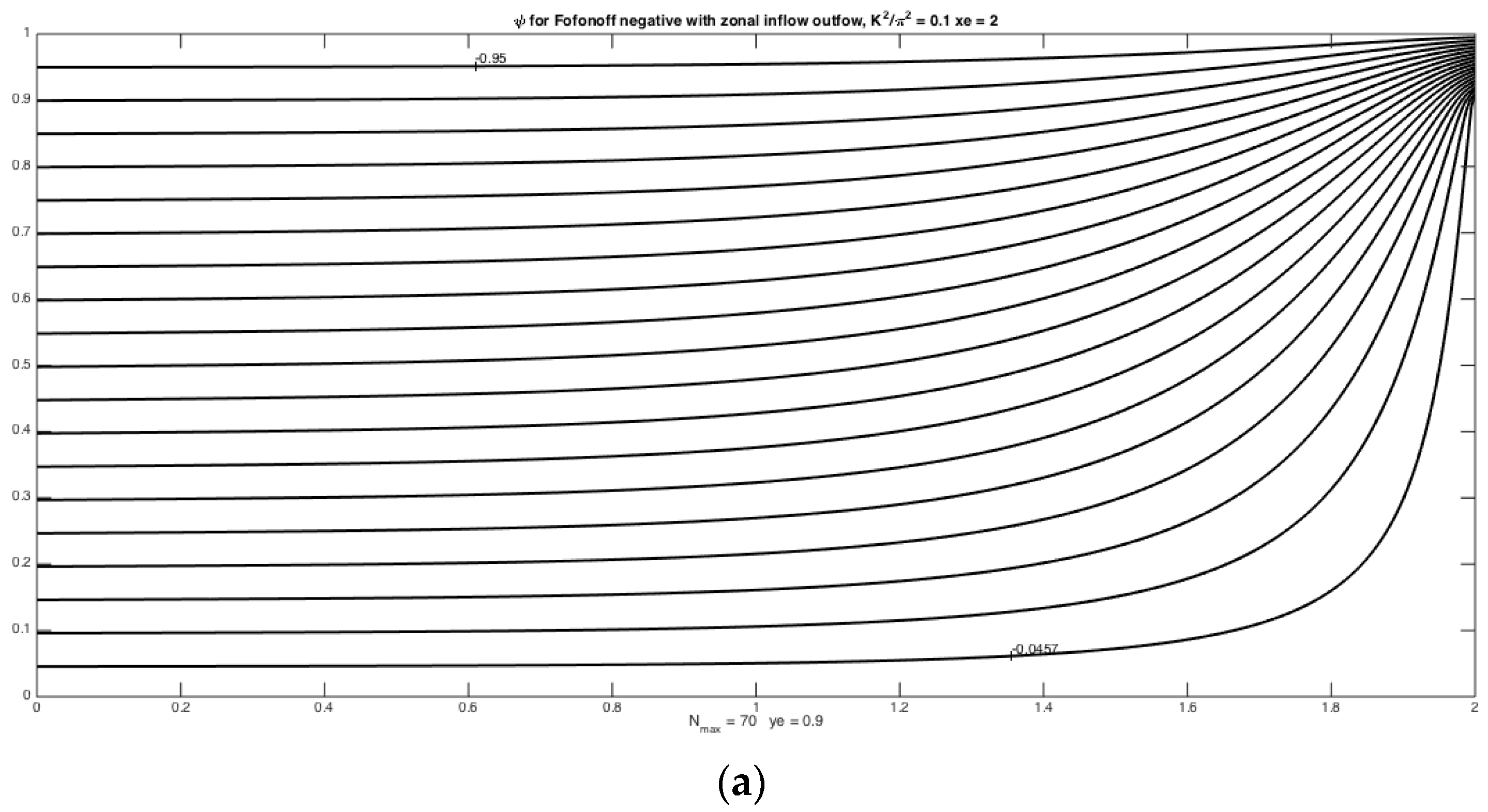
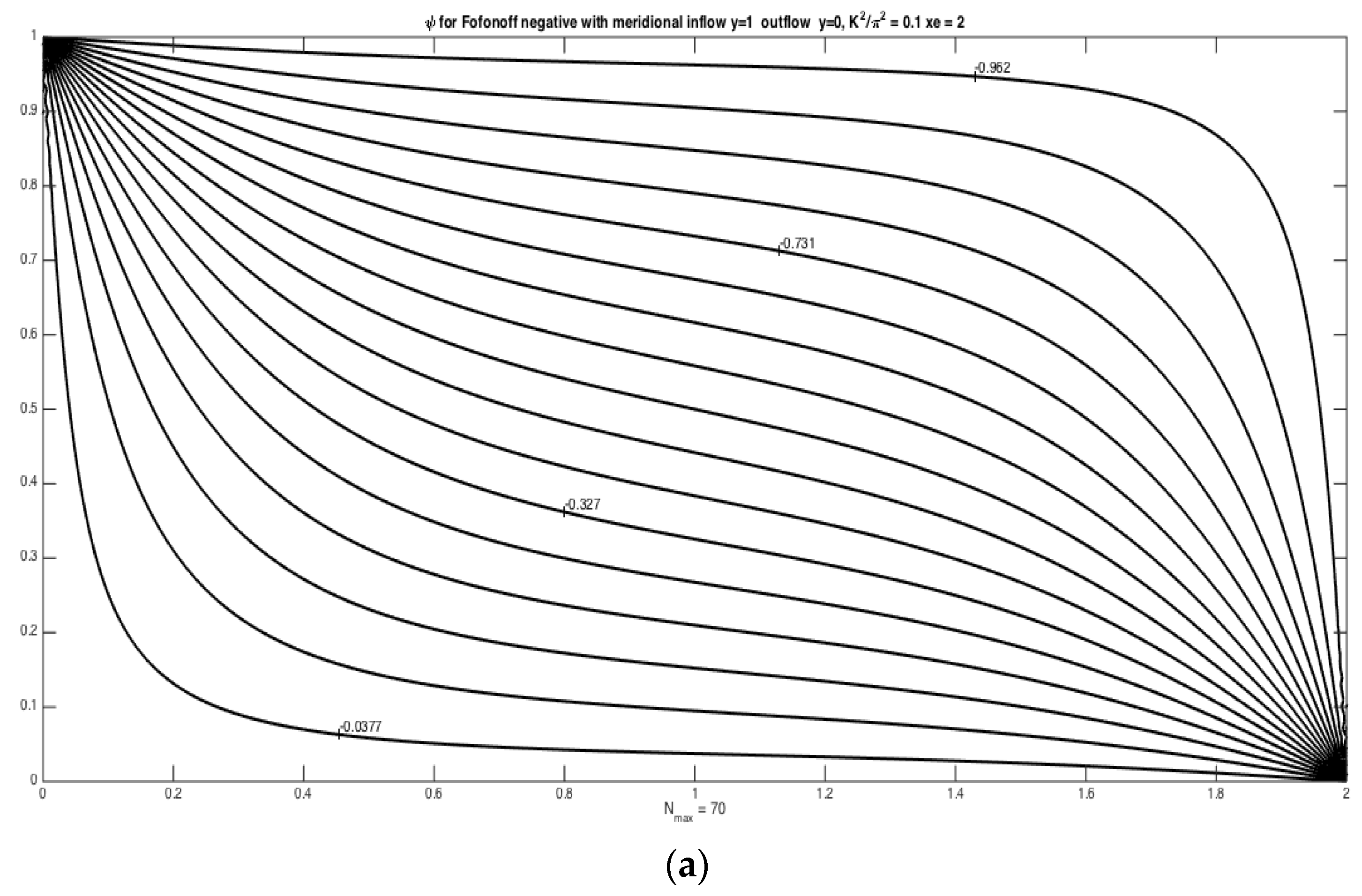
Figure 1 shows the solution for the problem in which the entering zonal flows leaves the region at the eastern boundary on $x=x_e=2$ in the restricted region for $y_e\le y\le 1$. Panel a shows the solution for $K^2/{\pi }^2=0.1$ so the solution is non-wavelike. The fluid moves smoothly from the entrance to exit region. 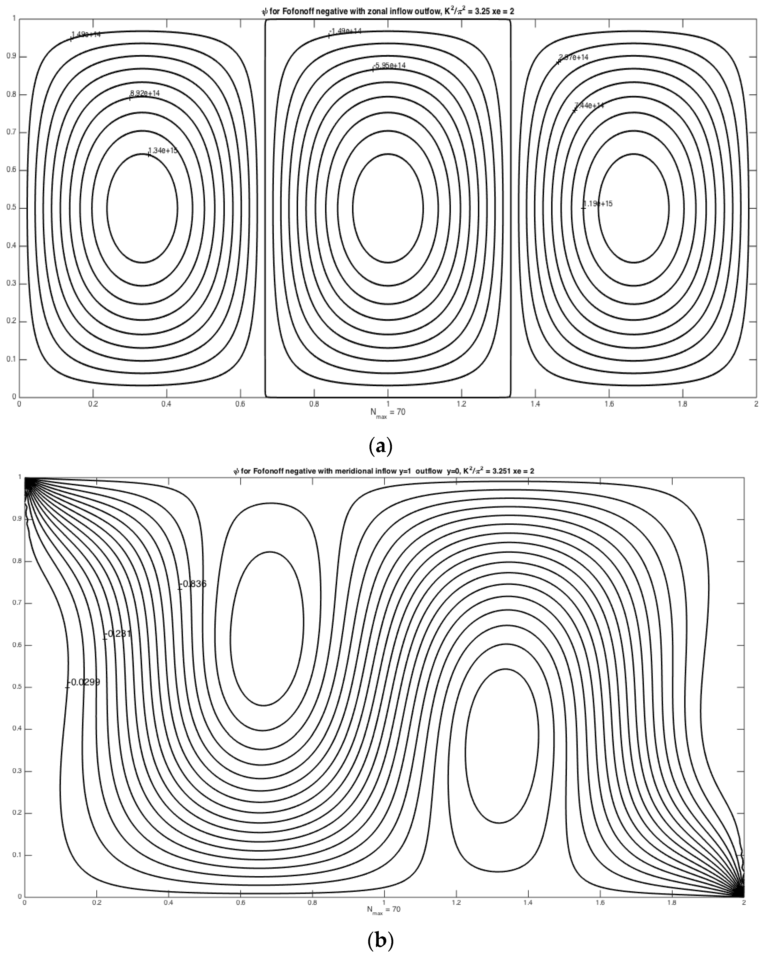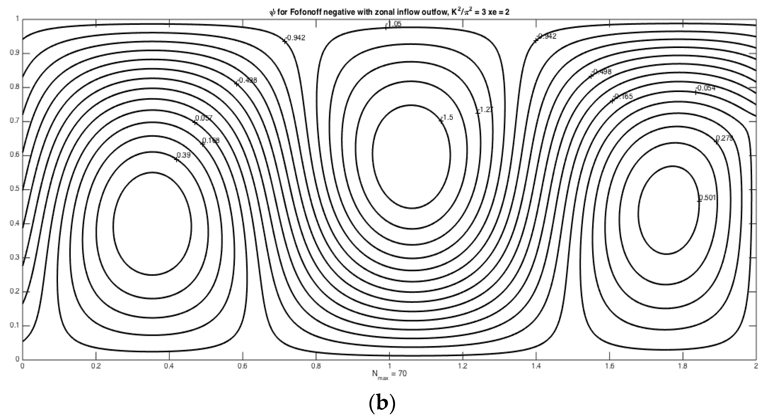Note that the relative vorticity in the solution is just given by $-K^2\phi$, and it is easy to show that the relative vorticity is localized near the exit region and is negative, i.e., anti-cyclonic. Panel b shows the solution in the wave regime for $K^2/{\pi }^2$ = 3.0 and demonstrates the appearance of a steady wave regime over the whole domain. One might think that the exiting flow would produce a zonal flow extending to the western boundary, but, in the absence of friction, no western boundary current on x = 0 is possible with interior eastward flow to join the inflow to a zonal interior current existing only in the region $y_e\le y\le 1$. That mismatch forces the production of a wavelike current connecting inflow and outflow. This is the basin-wide Rossby mode caused by an island interrupting an eastward zonal flow that was observed by P & S. Larger values of K² yield shorter wavelengths in x. Note that if the domain in Figure 1 were reflected about y = 0, the solution obtained above would represent the disturbed flow to the east of a narrow island at x = x_e.

The possibility of resonance will be discussed below, but it is clear, in this simple case, that it will occur whenever ${\alpha }_n{x}_e$ is an integral multiple of π.

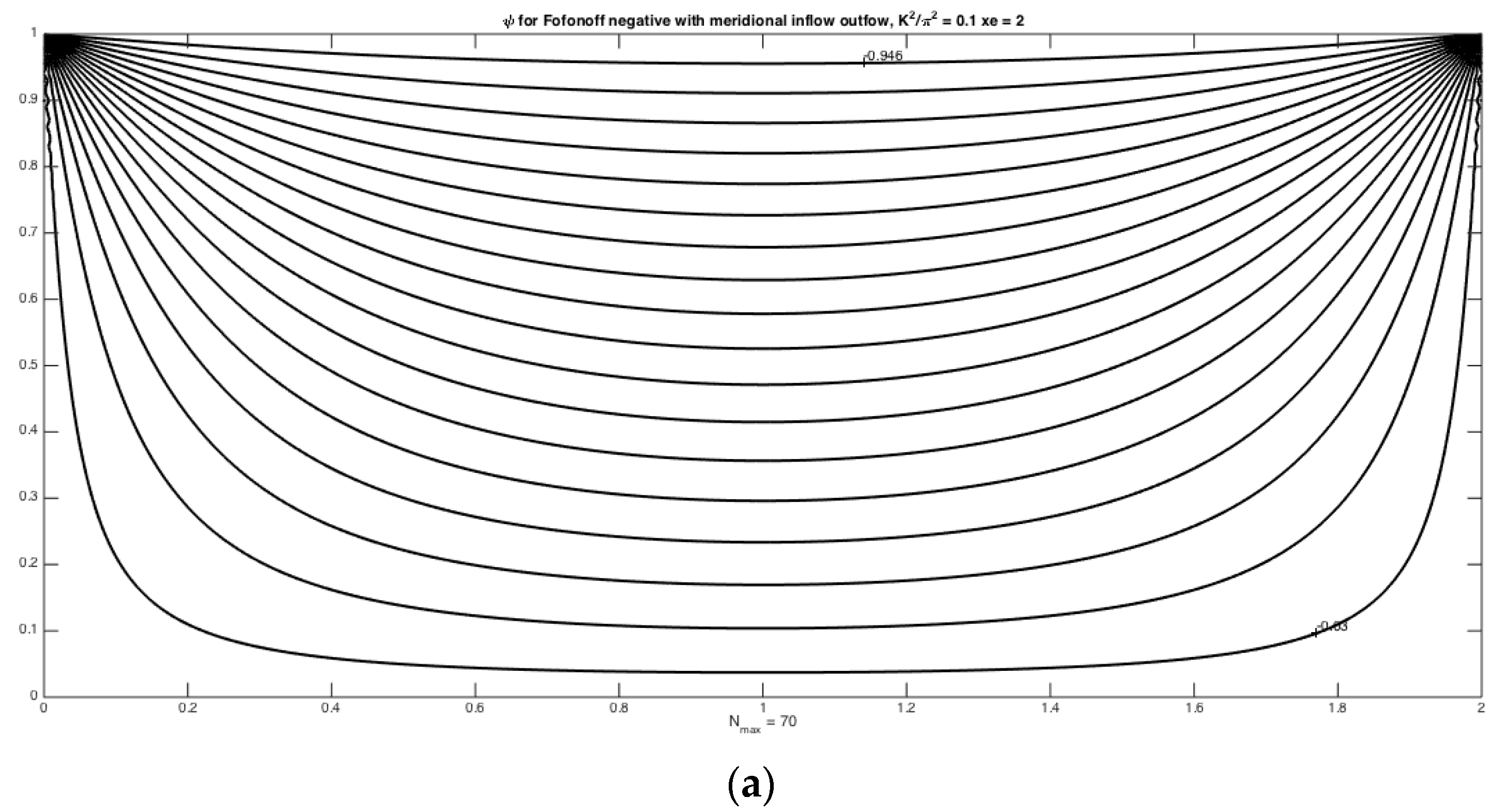
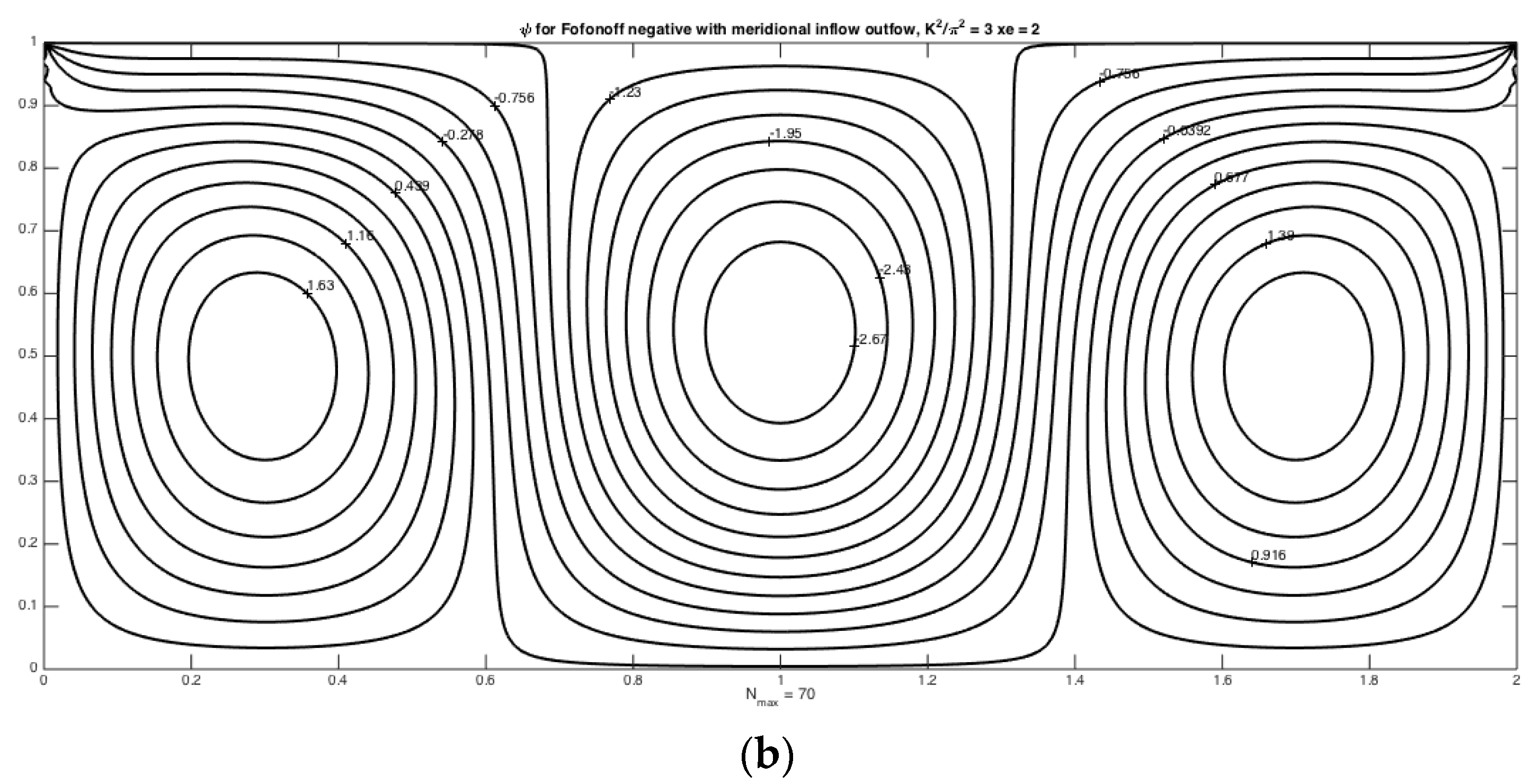
Example 2, which has the flow entering through a narrow gap in the northwest corner of the basin and exiting in a similar gap in the northeast corner, is represented by the solution,

$$\begin{array}{l}\psi ={\psi }_2=-y+{\phi }_2\\ {\phi }_2={\displaystyle \sum _{n=1}\frac{2{(-1)}^{n+1}}{n\pi }\left(\frac{\sin {\alpha }_{n}x}{\sin {\alpha }_n{x}_e}-\frac{\sin {\alpha }_n(x-x_e)}{\sin {\alpha }_n{x}_e}\right)}\sin n\pi y\end{array}.$$

(5)

The solution for this example is shown in Figure 2. As in Figure 1, panel a shows the flow for $K^2=0.1{\pi }^2$ so that no wave is possible and the flow enters and leaves smoothly generating relative vorticity wherever the flow deviates from a latitude circle (lines of constant y). Panel b demonstrates the wave-like solution naturally produced when $K^2/{\pi }^2$ is greater than one and we observe qualitatively the same solution as in Figure 1. Note that in both cases the predominant flow sustaining the wave is eastward and that the wave field occupies the full domain.

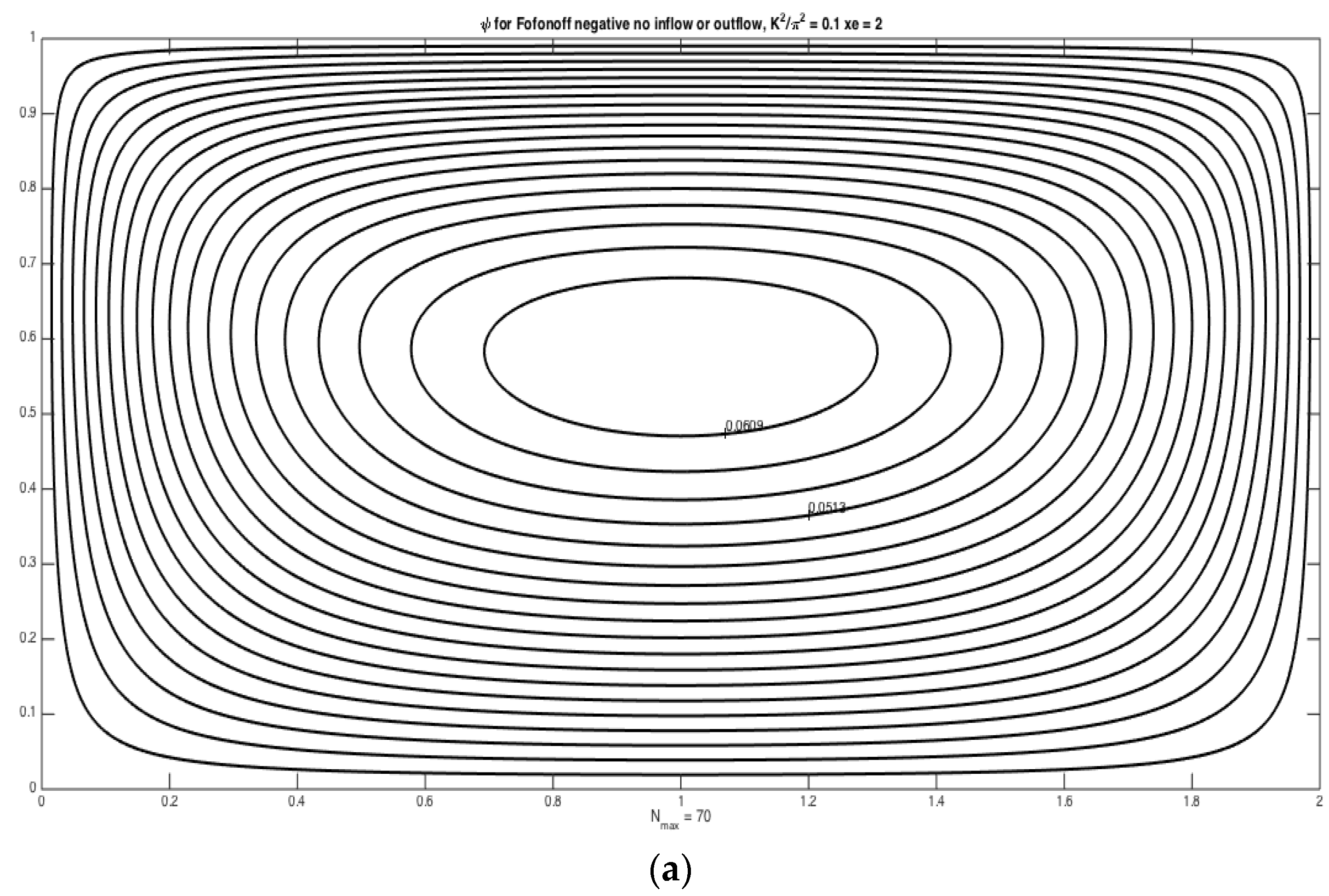
The third example is the solution to Equation (2) when there is no inflow or outflow and thus where ψ is zero on the entire basin boundary. This free mode follows from the search of nontrivial solution of the unforced vorticity equation with $\psi \ne 0$, as mentioned above. In this case, the solution is

$$\begin{array}{cc}\hfill \psi & ={\psi }_3\hfill \\ & =2{\displaystyle \sum _{n=1}\frac{{(-1)}^n{K}^2}{n\pi (K^2-n^2{\pi }^2)}\left[1-\frac{\sin {\alpha }_{n}x}{\sin {\alpha }_n{x}_e}+\frac{\sin {\alpha }_n(x-x_e)}{\sin {\alpha }_n{x}_e}\right]\sin n\pi y}\hfill \end{array}.$$

(6)

Note that, if $K^2$ were zero, the solution would be null. Figure 3a shows the solution for the small $K^2$ case (0.1) as in the previous examples. It demonstrates the essential aspect of the Fofonoff negative mode. There is a single anticyclonic cell with westward flow in the southern part of the basin and enhanced eastward flow in the northern latitudes, and that cell can be seen as what is needed to produce the intensified exit flow observed in Figure 1a. In Figure 3b, the 3-wave regime obtained in the first two examples is manifest and is clearly a feature of the pure, unforced, Fofonoff negative mode that becomes excited by the inflow/outflow forcing in the first two examples.

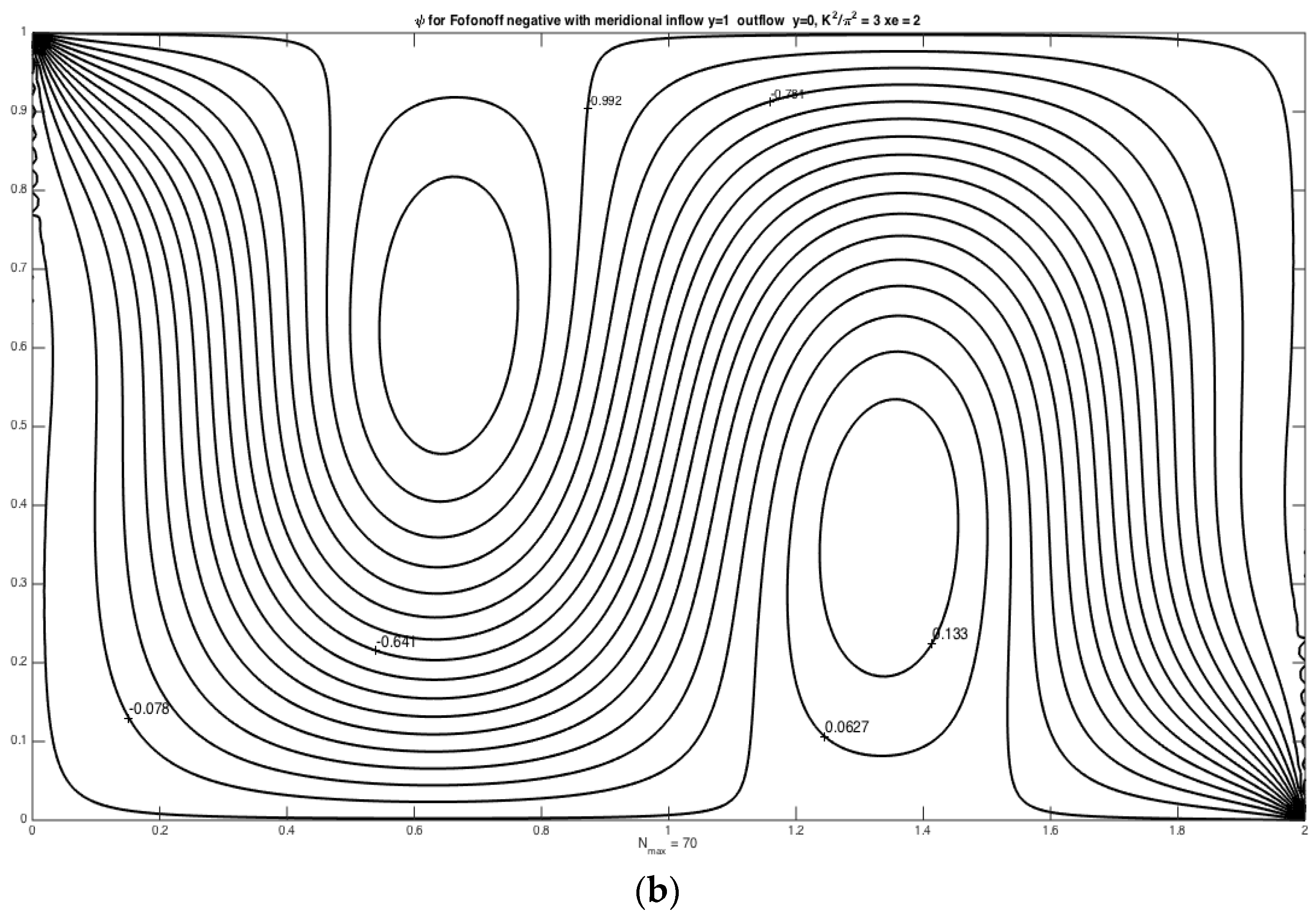
Finally, the solution for the fourth example, which has the same flux entering in the northwestern corner as in example two but has the flow leaving in the southeastern corner, is,

$$\begin{array}{l}\psi ={\psi }_4=-y+{\phi }_4,\\ {\phi }_4={\displaystyle \sum _{n=1}\left[\frac{-2}{n\pi }\frac{\sin {\alpha }_{n}x}{\sin {\alpha }_n{x}_e}+\frac{2{(-1)}^n}{n\pi }\frac{\sin {\alpha }_n(x-x_e)}{\sin {\alpha }_n{x}_e}\right]\sin n\pi y}\end{array}.$$

(7)

Figure 4 shows the solution Equation (7) for the same two values of $K^2$ as the previous three examples. The principal difference between example 2 and example 4 is the difference in symmetry in x of the streamline pattern, and this has important consequences for the issue of resonance as discussed in the next section.

3. Resonance

It is clear from the above solutions that a necessary condition for resonance is that ${\alpha }_n{x}_e=j\pi$, where j is an integer for some n in the sums on n. This would yield an integral number of wave oscillations in the interval (0, x_e). However, this is generally not a sufficient condition for resonance in all four of the cases described above.

It is for the first problem, though, whose solution is Equation (4). Any value of K such that

$$\frac{K^2}{{\pi }^2}=n^2+\raisebox{1ex}{$j^2$}\!\left/ \!\raisebox{-1ex}{${x_e}^2$}\right.$$

(8)

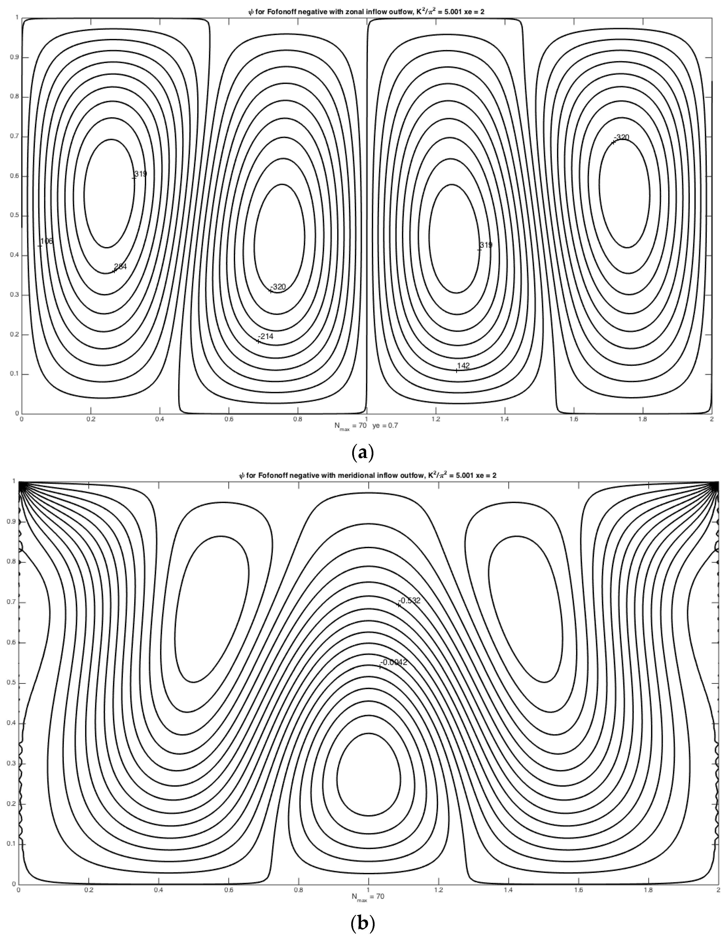
for some n and integer j leads to resonance with ${\alpha }_n{x}_e=j\pi$. We can reveal the form of the solution by choosing a value of K very near the value given by Equation (8). Thus, for example, if n = 1 and j = 4 for x_e = 2, resonance occurs when $K^2/{\pi }^2$ = 5. Figure 5a shows the solution for a value of $K^2/{\pi }^2$ very near resonance, i.e., at $K^2/{\pi }^2$ = 5.001. The solution appears to be a pure standing wave and the amplitude of the wave is very large, so much greater than O(1) that the inflow and outflow streamlines that force the solution are not evident. Note that Figure 5b shows a solution that is qualitatively similar to Figure 2b. The entering and exiting streamlines are evident and the amplitude of the excited wave is O(1). In fact, each of the solutions 2 through 4 are non-resonant.

The reason for the non-resonance of the other solutions follows from their symmetries. For example, in problem 2 with the meridional inflow and outflow, the solution in Equation (5) would be resonant for K satisfying Equation (8) unless the numerator of the combined terms is zero. The numerator may be rewritten,

$$\begin{array}{cc}\hfill \sin {\alpha }_{n}x-\sin {\alpha }_n(x-x_e)& =\sin {\alpha }_{n}x\left(1-\cos {\alpha }_n{x}_e\right)+\sin {\alpha }_n{x}_e\cos {\alpha }_{n}x\hfill \\ & =\sin {\alpha }_{n}x(1-{(-1)}^j)+0\hfill \end{array}.$$

(9)

Thus, if j is even, as in the example, the numerator would be zero at the resonance value of K and the solution to the second problem remains regular at that value of K. Resonance for the problem of the meridional inflow/outflow at y = 1 requires a value of K that allows values of j that are odd. It is not hard to show that this is also true for problem 3, i.e., Equation (6). For the problem with inflow at the western corner at y =1 and outflow at the eastern corner at y = 0, it is not difficult to see that resonance for values of n and j requires that the sum, n + j, must be an odd number.

To illustrate that fact, Figure 6a shows the resonant form of the solution for all the problems except problem 4, the case requiring that n + j be odd. In the example shown, $K^2/{\pi }^2=3.25$ corresponding to n = 1, j = 3. The solution corresponds to a free stationary wave with three oscillations in the x interval, and this resonant form holds for all the examples except problem four because now n + j = 4 and is even. The example for that problem for this value of K is shown in Figure 6b and is clearly non-resonant.

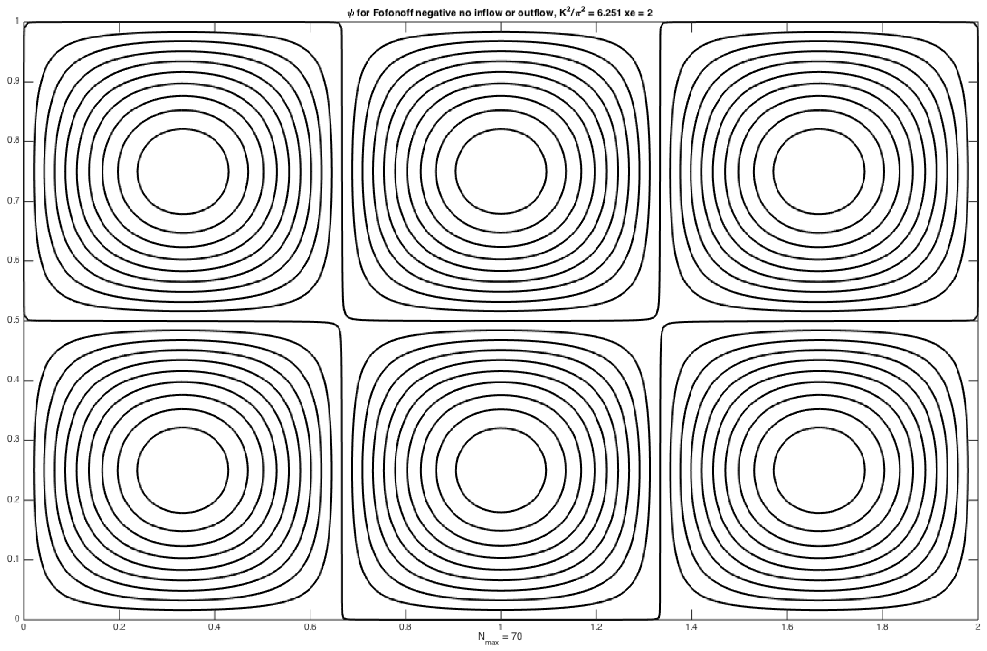
Figure 7 shows the form of the solution for all cases when $K^2/{\pi }^2$ is 6.251, the near resonance case corresponding to n = 2, j = 3 and x_e = 2. Since j is odd and n + j is also odd, each of the four solutions is resonant. Again, the magnitude of the solution at resonance is so large that the details of the forcing inflows and outflows become negligible compared to the free wave excited by the response.

4. Discussion and Conclusions

When the dynamics under consideration has negligible frictional dissipation and no external forcing, one might anticipate that the steady vorticity equation

$$J(\psi ,{\nabla }^2\psi +\beta y)=0$$

(10)

would be an appropriate governing equation over most of the domain. If so, it follows that the solution must have the form Equation (1), i.e., the total vorticity must be constant on streamlines. The determination of the functional relation in Equation (2), i.e., the function $Q(\psi )$ is often problematic. If the flow is driven by an inflow condition as given by Equaion (3a), one can determine $Q(\psi )$ as given by Equation (2) on those streamlines connected directly to the inflow, that is, on streamlines that can be traced back to the entrance region. When the streamlines are closed in the interior, it is less certain what the $Q(\psi )$ relationship should be for those streamlines. In the absence of forcing, friction, when small, could homogenize the total vorticity as suggested by Batchelor’s theorem [5]. Other small sources of dissipation or forcing could also modify the relationship for large time. Nevertheless, Equation (2) is certainly a solution to the inviscid problem and is analogous with the usual Fofonoff solution, which also has closed streamlines and could be excited in cases where the dissipation is not large enough to prevent inertial runaway. The difference from the conventional situation is that here the interior flow is largely eastward so no inertial boundary layers are possible, and the energy that would be confined to such boundary layers for westward interior flow is instead permitted to radiate into the basin interior. This seems to be the explanation for the widespread wave response in the island problem discussed by P & S.

An important difference between the traditional Fofonoff mode and the Fofonoff negative mode is that since $\raisebox{1ex}{$dQ$}\!\left/ \!\raisebox{-1ex}{$d\psi $}\right.<0$, it satisfies the necessary condition for instability [6]. Especially for large K, time dependent instabilities can be anticipated as a form of Rossby wave instability. Since any such instability requires energy to flow to larger scales as well as smaller scales, the solutions for values of $\raisebox{1ex}{$K^2$}\!\left/ \!\raisebox{-1ex}{${\pi }^2$}\right.$ slightly greater than unity may remain stable. It will be of interest to examine that possibility in future work.