An Hourly Operational Dataset of Grid-Connected and Islanded Green-Power Chemical Parks for Flexible Production and Safety Power Supply

Abstract

The deep decarbonization of high-emission chemical industries requires green hydrogen–ammonia parks that directly integrate volatile renewable energy with continuous synthesis processes. However, high-resolution, physically consistent operational datasets covering the multi-stage evolution from grid-connected economic dispatch to off-grid resilient islanded operation remain scarce. This paper presents a comprehensive, multi-scenario operational dataset for a green-power, directly connected hydrogen–ammonia chemical park in Jilin, Northern China. Derived from 24 typical meteorological scenarios, the dataset covers grid-connected mode with five daily ammonia production targets (72–36 tons/day) and off-grid mode with dynamic yield maximization under a 195 MWh battery energy storage system. Hourly records are provided for renewable generation, electrolyzer and synthesis unit power consumption, grid exchange, battery state-of-charge, and waste heat recovery. All operational states are strictly validated against physical constraints—equipment load limits, energy conservation laws, thermodynamic recovery bounds, and state-of-charge limits—ensuring engineering feasibility. The dataset is publicly available in CSV format and serves as a benchmark for capacity planning, energy management system development, and flexible production strategy validation.

Dataset: https://github.com/Data-provider2026/Hourly-Grid-Connected-and-Islanded-Operation-Dataset-for-the-Green-Chemical-Park (accessed on 20 June 2026).

Dataset License: CC-BY Attribution 4.0 International

1. Introduction

The global transition toward sustainable energy systems necessitates the deep decarbonization of high-emission heavy industries. Green-power, directly connected hydrogen–ammonia chemical parks have emerged as a critical pathway to absorb large-scale variable renewable energy while producing zero-carbon fuels and chemicals [1,2,3]. By replacing traditional fossil-based synthesis processes with renewable-driven electrolysis and flexible synthesis loops, these multi-energy parks play a vital role in collaborative decarbonization. However, the direct coupling of highly volatile wind and solar power with stringent, continuous chemical processes introduces severe operational challenges [4,5].

Unlike conventional power systems, chemical parks require a strict safety power supply to maintain thermodynamic stability and prevent costly or hazardous process shutdowns. The variable nature of renewable energy creates a mismatch with the continuous load demands of chemical synthesis. To address this, modern green-power parks utilize complex electro-thermal coupling technologies—coordinating multi-state electrolyzers (e.g., Alkaline and PEM), flexible ammonia synthesis units (AMU), electric boilers (EB), and waste heat recovery units (WHRU) [6,7,8]. Recent studies have further explored the nonlinear predictive regulation of such integrated systems under time-varying renewable supply [9], as well as the thermoeconomic potential of multi-generation configurations producing hydrogen, ammonia, and methanol simultaneously [10]. Balancing these dynamic renewable generation inputs with rigid chemical production constraints requires precise, multi-timescale energy management.

Despite the growing theoretical interest in green hydrogen–ammonia synergies, a critical gap remains in the availability of high-resolution, physically bounded, and scenario-comprehensive operational datasets. Existing open-access energy datasets predominantly focus on generalized power grids or single-source renewable profiles, largely overlooking the intricate energy-mass flow constraints and thermodynamic limits inherent to chemical facilities [11,12]. More importantly, current databases fail to capture the multi-stage operational evolution of these systems: from near-term grid-connected architectures aimed at economic interaction and collaborative decarbonization, to long-term off-grid islanded modes designed for dynamic yield maximization and continuous safety power supply under extreme weather scenarios [13]. While recent optimization frameworks have advanced the design and scheduling of hydrogen–ammonia systems [14], they often rely on hypothetical or reduced-order models, underscoring the pressing need for high-fidelity, physically consistent operational data. This absence significantly limits the development and validation of advanced multi-energy system modeling and specialized algorithms.

To bridge these gaps, this paper presents a comprehensive, multi-scenario operational dataset for green-power, directly connected hydrogen–ammonia parks. The fundamental meteorological data and baseline operational parameters were collected from a real-world green-power, directly connected hydrogen–ammonia chemical park located in Jilin, Northern China. This region is characterized by abundant wind–solar resources and specific seasonal weather patterns, providing a unique environment to collect data on multi-state electrolyzer (ALKEL-PEMEL) synergistic operation and islanded resilience. Driven by 24 typical meteorological scenarios extracted from the site, the dataset employs exact physics-based models to generate high-fidelity, hourly operation records. By distinctly separating the data into a Grid-Connected Park Operation Dataset and an Off-Grid Park Operation Dataset, it provides a complete evolutionary trajectory of the system. The dataset rigorously enforces physical operating boundaries—incorporating electrolyzer ramp rates, AMU thermal coefficients, and natural heat dissipation constraints—ensuring that all simulated outputs, power deficits, and curtailment records are directly applicable to practical engineering. Beyond the dataset itself, two practical application cases are included to demonstrate its value: one covering hybrid capacity planning and technical parameter validation, and another demonstrating its utility as a benchmark for developing multi-energy coupled dispatch algorithms and flexible production control.

The main contributions of this work can be summarized as follows:

• Development of a high-resolution, multi-scenario operational dataset specifically designed for green-power, directly connected hydrogen–ammonia chemical parks.
• Integration of complex electro-thermal coupling and multi-state hydrogen production models (ALKEL/PEMEL synergy) to ensure physically bounded and mathematically exact power-to-chemical generation records.
• Provision of a dual-stage evolutionary data framework, capturing both grid-connected collaborative decarbonization (economic dispatch) and off-grid safety power supply (dynamic yield and resilience) operations.
• Demonstration of dataset applicability in advanced engineering applications, providing a reliable benchmark for capacity sizing, parameter validation, and data-driven energy management system (EMS) algorithm development.

Overall, this dataset establishes a robust and physically consistent foundation for researching the transition of high-emission chemical industries toward zero-carbon, flexible production. By offering a rigorous, multi-stage operational benchmark, it empowers researchers and engineers to tackle the complex electro-thermal coordination and safety power supply challenges inherent to the modern energy-chemical nexus. The remainder of this paper is organized as follows: Section 2 details the data file structures and multi-scenario operational records. Section 3 elaborates on the physics-based mathematical models and the multi-stage evolutionary dispatch strategies. Section 4 presents a thorough data exploration and technical evaluation. Section 5 discusses advanced user applications, and finally, Section 6 concludes the paper.

2. Data Description

This dataset provides a high-resolution, multi-scenario collection of operational records for green-power, directly connected hydrogen–ammonia chemical parks. The foundational meteorological profiles and system baseline limits were directly collected from an actual green hydrogen–ammonia park in Jilin, Northern China. Instead of evaluating a single continuous timeline, the dataset is driven by 24 typical meteorological scenarios recorded at the site to capture the system’s performance under the characteristic renewable volatility of this region. The data maintains a strict hourly time resolution, resulting in 24 h of operational data for each of the 24 scenarios.

To clearly decouple the physical environmental inputs from the complex electro-thermal synergistic responses under different system architectures (grid-tied vs. islanded), the entire dataset is systematically divided into three separate sub-datasets. All information is archived in CSV format utilizing UTF-8 encoding, ensuring that the files can be processed safely on any operating system (Windows, macOS, or Linux) and easily imported into programming environments like MATLAB or Python for further algorithmic validation.

2.1. Base Scenario Dataset

The first sub-dataset provides the fundamental environmental metrics and the foundational load demands of the chemical park. This file is named Scenarios_Base_Data.csv. It establishes the physical baseline that drives the subsequent multi-energy dispatch models. The detailed explanations of the six variables are as follows:

• Scenario_ID: This is the identifier assigned to each meteorological scenario, numbered from 1 to 24. It represents 24 different typical wind–solar scenarios used to test the system’s operational performance.
• Hour: This represents the exact hour of the day, presented in a standard 24 h format ranging from 1 to 24.
• Base_Elec_Load_MW: The foundational conventional electrical load of the chemical park, measured in Megawatts (MW).
• Base_Thermal_Load_MW: The foundational thermal heating demand of the chemical park, measured in MW.
• Wind_Power_MW: The available wind power generation under the specific scenario, measured in MW.
• Solar_Power_MW: The available solar photovoltaic (PV) power generation under the specific scenario, measured in MW.

To provide a clear understanding of the baseline inputs,

Table 1. Example data in the Base Scenario Dataset (Sample from Scenario 1).

Scenario_ID	Hour (h)	Base_Elec_Load_MW	Base_Thermal_Load_MW	Wind_Power_MW	Solar_Power_MW
1	1	1.3698	3.1934	9.7760	0.0000
1	2	1.0998	3.2728	10.9040	0.0000
1	3	0.7998	3.3187	15.1520	0.0000

presents an actual data sample showing the first three hours of Scenario 1.

2.2. Grid-Connected Operation Dataset

The second sub-dataset translates the base scenarios into actual electro-thermal synergistic operations under a grid-connected architecture. Named Gridconnected_Park_Operation_Data.csv, it records the precise power allocation across multi-state chemical equipment to meet varying daily ammonia production targets. Five production targets are considered: 72, 63, 54, 45, and 36 tons/day. The key variables include:

• Yield_Target_ton: The step-wise daily green ammonia production target, decreasing from 72 tons to 36 tons. This variable drives the flexible production dispatch.
• Scenario_ID: The identifier assigned to each meteorological scenario, numbered from 1 to 24, representing different typical wind–solar scenarios.
• Hour: The exact hour of the day in a standard 24 h format ranging from 1 to 24.
• Wind_Power_MW and Solar_Power_MW: The available wind and solar photovoltaic (PV) power generation under the specific scenario, measured in MW.
• Total_Elec_Load_MW: The total system electrical load (MW), which accurately aggregates the base load, electrolyzers, ammonia synthesis units (AMU), and electric boilers (EB).
• Grid_Buy_MW and Grid_Sell_MW: The amount of power purchased from or sold to the main grid (MW) to maintain chemical process stability and maximize economic benefits.
• Thermal_Load_MW: The physical thermal load requirement of the park (MW).
• EB_Power_MW: The electrical power consumed by the Electric Boiler (MW) to generate heat.
• WHRU_Heat_MW: The thermal energy (MW) recovered by the Waste Heat Recovery Unit (WHRU) from the electrolysis and exothermic synthesis processes.
• ALKEL_Power_MW and PEMEL_Power_MW: The electrical power allocated to the Alkaline and Proton Exchange Membrane electrolyzers (MW), reflecting their distinct ramp rates and synergistic operation.
• AMU_Power_MW: The power consumed by the flexible Ammonia Synthesis Unit (MW).

A sample of this dataset is presented in

Table 2. Example data in the Grid-Connected Operation Dataset (Target: 72 tons, Scenario 1)—Part 1.

Yield_Target	Scenario_ID	Hour	Wind_Power	Solar_Power	Total_Load	Grid_Buy	Grid_Sell
72	1	1	9.7760	0.0000	42.8698	33.0938	0.0000
72	1	2	10.9040	0.0000	42.5998	31.6958	0.0000
72	1	3	15.1520	0.0000	42.2998	27.1478	0.0000

and

Table 3. Example data in the Grid-Connected Operation Dataset (Target: 72 tons, Scenario 1)—Part 2.

Thermal_Load	EB_Power	WHRU_Heat	ALKEL_Power	PEMEL_Power	AMU_Power
3.1934	0.0000	3.1934	20.0000	20.0000	1.5000
3.2729	0.0000	3.2729	20.0000	20.0000	1.5000
3.3187	0.0000	3.3187	20.0000	20.0000	1.5000

, illustrating the multi-energy allocation for a 72 ton target under Scenario 1. Due to the large number of variables, the table is split into two parts.

2.3. Off-Grid Operation Dataset

The third sub-dataset characterizes the system’s resilience and safety power supply capabilities during completely islanded operations. Named Offgrid_Park_Operation_Data.csv, it captures the dynamic yield maximization strategy under extreme weather, constrained by a fixed 195 MWh Battery Energy Storage System (BESS). The variables in this file include:

• Scenario_ID: The identifier assigned to each meteorological scenario, numbered from 1 to 24, representing different typical wind–solar scenarios.
• Hour: The exact hour of the day in a standard 24 h format ranging from 1 to 24.
• Wind_Power_MW and Solar_Power_MW: The available wind and solar photovoltaic (PV) power generation under the specific scenario, measured in MW.
• Base_Elec_Load_MW: The foundational conventional electrical load of the chemical park, measured in MW.
• ALKEL_Power_MW, PEMEL_Power_MW, and AMU_Power_MW: The electrical power consumed by the Alkaline electrolyzer, Proton Exchange Membrane electrolyzer, and flexible Ammonia Synthesis Unit, respectively, measured in MW.
• BESS_Charge_MW and BESS_Discharge_MW: The power (MW) charged into or discharged from the BESS to buffer renewable volatility and support the continuous chemical load.
• Curtailment_MW: The excess renewable power (MW) that could not be stored or utilized by the flexible chemical processes.
• Power_Deficit_MW: The unserved load or power deficit (MW). This is a critical metric utilized to assess safety power supply boundaries, revealing instances where the islanded system fails to sustain operations.
• BESS_SOC_Percentage: The State of Charge (SOC) of the battery system, reflecting the real-time energy reserve level.
• Thermal_Load_MW: The physical thermal load requirement of the park (MW).
• EB_Power_MW: The electrical power consumed by the Electric Boiler (MW) to generate heat.
• WHRU_Heat_MW: The thermal energy (MW) recovered by the Waste Heat Recovery Unit (WHRU) from the electrolysis and exothermic synthesis processes.

By enforcing rigorous physical boundaries and thermodynamic limits throughout the modeling process, these datasets effectively eliminate invalid operational states, providing a highly reliable engineering benchmark. A sample of the off-grid resilience response is provided in

Table 4. Example data in the Off-Grid Operation Dataset (Scenario 1)—Part 1.

Scenario_ID	Hour	Wind_Power	Solar_Power	Base_Load	ALKEL_Power	PEMEL_Power	AMU_Power
1	1	9.7760	0.0000	1.3698	20.0000	6.5351	0.9614
1	2	10.9040	0.0000	1.0998	20.0000	0.0000	0.7000
1	3	15.1520	0.0000	3.7998	20.0000	0.0000	0.7000

and

Table 5. Example data in the Off-Grid Operation Dataset (Scenario 1)—Part 2.

BESS_Chg	BESS_Dis	Curtailment	Deficit	SOC(%)	Thermal_Load	EB_Power	WHRU_Heat
19.0903	0.0000	0.0000	0.0000	49.11	3.1934	0.0000	3.1934
10.8958	0.0000	0.0000	0.0000	42.89	3.2729	0.0000	3.2729
6.3478	0.0000	0.0000	0.0000	39.27	3.3187	0.0000	3.3187

, split into two parts due to the number of variables.

3. Methodology and Physical Models

This section presents the comprehensive mathematical framework underpinning the dataset generation process. The methodology is structured around two distinct operational paradigms: grid-connected mode, which enables economic dispatch with external grid interaction, and off-grid mode, which enforces autonomous islanded operation with battery energy storage. All models are built upon first-principle physics, ensuring that the generated dataset is physically consistent, thermodynamically feasible, and directly applicable to engineering practice.

3.1. System Architecture Overview

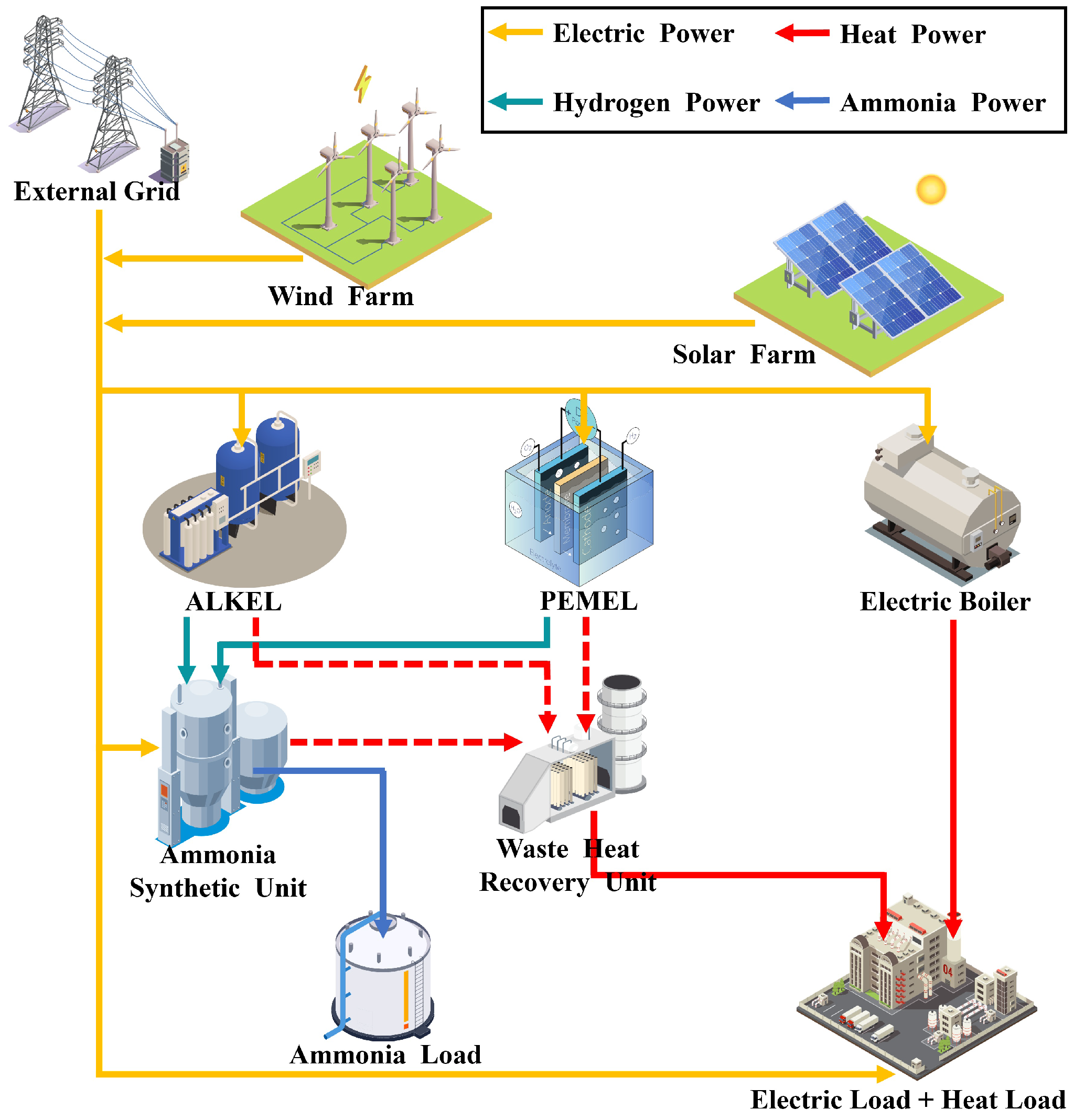
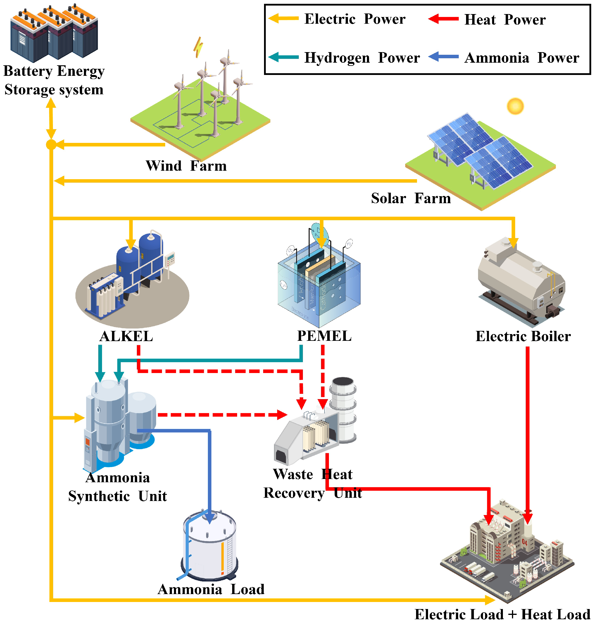
The investigated green hydrogen–ammonia park comprises four functional domains: renewable energy supply, power-to-hydrogen conversion, ammonia synthesis, and thermal energy management. The system architecture for both operational modes is illustrated in Figure 1 and Figure 2.

The investigated green hydrogen–ammonia park is located in Jilin Province, northeastern China, a region characterized by abundant wind–solar resources with distinct seasonal variations. The park integrates three functional domains: renewable generation (40 MW wind + 64 MW PV), power-to-hydrogen conversion (20 MW ALKEL + 20 MW PEMEL), and ammonia synthesis (1.5 MW AMU). Key equipment parameters are summarized in Appendix A,

Table A1. Equipment specifications and physical parameters.

Group 1				Group 2
Symbol	Description	Value	Unit	Symbol	Description	Value	Unit
$P_{\mathrm{WT}}^{\mathrm{rated}}$	Wind farm rated capacity	40	MW	${\lambda }_{\mathrm{AMU}}^{\mathrm{e}}$	AMU electricity consumption coefficient	0.0005	MWh/kg NH3
$P_{\mathrm{PV}}^{\mathrm{rated}}$	Solar PV rated capacity	64	MW	${\lambda }_{\mathrm{AMU}}^{\mathrm{h}}$	AMU heat release coefficient	0.0003	MWh/kg NH3
$P_{\mathrm{ALKEL}}^{\mathrm{rated}}$	ALKEL rated power	20	MW	${\eta }_{\mathrm{rec}}$	WHRU recovery efficiency coefficient	0.80	–
$P_{\mathrm{PEMEL}}^{\mathrm{rated}}$	PEMEL rated power	20	MW	${\eta }_{\mathrm{EB}}$	EB conversion efficiency coefficient	0.95	–
$P_{\mathrm{AMU}}^{\mathrm{rated}}$	AMU rated power	1.5	MW	$S_{\mathrm{ES}}$	BESS rated capacity	195	MWh
$P_{\mathrm{EB}}^{\mathrm{rated}}$	Electric boiler rated power	4	MW	${\eta }_{\mathrm{power}}$	BESS power-to-capacity ratio	0.50	–
${\eta }_{\mathrm{ALKEL}}$	ALKEL efficiency coefficient	0.70	–	${\eta }_{\mathrm{cha}}$	BESS charging efficiency	0.90	–
${\eta }_{\mathrm{PEMEL}}$	PEMEL efficiency coefficient	0.80	–	${\eta }_{\mathrm{dis}}$	BESS discharging efficiency	0.90	–
${\eta }_{\mathrm{ALKEL}}^{\min }$	ALKEL minimum load rate	0.10	–	${\eta }_{\mathrm{self}}$	BESS self-discharge rate	0.0002	–
${\eta }_{\mathrm{PEMEL}}^{\min }$	PEMEL minimum load rate	0.10	–	${\eta }_{\mathrm{SOC}}^{\min }$	BESS minimum SOC limit	0.10	–
${\eta }_{\mathrm{AMU}}^{\min }$	AMU minimum load rate	0.10	–	${\eta }_{\mathrm{SOC}}^{\max }$	BESS maximum SOC limit	0.90	–
${\lambda }_{\mathrm{ALKEL}}^{\mathrm{rated}}$	ALKEL rated electricity consumption coefficient	0.05	MWh/Nm3	${\eta }_{\mathrm{SOC}}^{\mathrm{ord}}$	BESS initial SOC coefficient	0.60	–
${\lambda }_{\mathrm{PEMEL}}^{\mathrm{rated}}$	PEMEL rated electricity consumption coefficient	0.05	MWh/Nm3	$M_1$	Big-M constant for buy/sell mutual exclusivity	${10}^{10}$	–
${\lambda }_{\mathrm{AMU}}^{{\mathrm{H}}_2}$	AMU hydrogen consumption coefficient	0.20	kgH2/kgNH3	$M_2$	Big-M constant for curtailment/deficit penalty	${10}^{10}$	–

,

Table A2. Economic parameters and cost coefficients.

Group 1				Group 2
Symbol	Description	Value	Unit	Symbol	Description	Value	Unit
$c_{\mathrm{WT}}^{\mathrm{LCOE}}$	Wind LCOE	150	RMB/MWh	$c_{\mathrm{WHRU}}^{\mathrm{OM}}$	WHRU O&M cost coefficient	5	RMB/MWh
$c_{\mathrm{PV}}^{\mathrm{LCOE}}$	Solar PV LCOE	120	RMB/MWh	$c_{\mathrm{EB}}^{\mathrm{OM}}$	EB O&M cost coefficient	15	RMB/MWh
$c_{\mathrm{ALKEL}}^{\mathrm{OM}}$	ALKEL O&M cost coefficient	100	RMB/MWh	$c_{\mathrm{ES}}^{\mathrm{OM}}$	BESS O&M cost coefficient	10	RMB/MWh
$c_{\mathrm{PEMEL}}^{\mathrm{OM}}$	PEMEL O&M cost coefficient	150	RMB/MWh	$p_{\mathrm{AM}}$	Green ammonia selling price	3800	RMB/ton
$c_{\mathrm{AMU}}^{\mathrm{OM}}$	AMU O&M cost coefficient	2	RMB/MWh	$c_{\mathrm{sell}}$	Renewable energy feed-in tariff	377.9	RMB/MWh

and

Table A3. Time-of-use electricity purchase prices.

Period Type	Time Slots	Price
Valley	1:00–7:00, 23:00–24:00	342.4 RMB/MWh
Shoulder	8:00–10:00, 15:00–16:00, 20:00–22:00	607.4 RMB/MWh
Peak	11:00–14:00, 17:00–19:00	802.4 RMB/MWh

.

The renewable generation side consists of a 40 MW wind turbine (WT) farm and a 64 MW solar photovoltaic (PV) station. The power-to-hydrogen conversion stage comprises two complementary electrolysis technologies: an Alkaline Electrolyzer (ALKEL) rated at 20 MW with a hydrogen yield of 280 Nm³/h, and a Proton Exchange Membrane Electrolyzer (PEMEL) rated at 20 MW with a hydrogen yield of 320 Nm³/h. The ammonia synthesis unit (AMU) operates at 1.5 MW rated power, consuming 600 Nm³/h of hydrogen at full load. Thermal integration is achieved through a Waste Heat Recovery Unit (WHRU) with 80% recovery efficiency and an Electric Boiler (EB) with 4 MW capacity and 95% conversion efficiency. In off-grid mode, a 195 MWh Battery Energy Storage System (BESS) is introduced with a power-to-capacity ratio of 0.5, charge/discharge efficiency of 90%, and state-of-charge limits of 10% to 90%.

All key parameters with their symbols, values, and units are consolidated in Appendix A, Table A1, Table A2 and Table A3, for reference.

3.2. Grid-Connected Multi-Energy System Modeling

3.2.1. Renewable Generation Dispatch and Grid Interaction

For the grid-connected mode, the renewable generation is split into two streams: direct supply to the park and feed-in to the external grid. The power balance for wind and solar generation is expressed as:

$$P_{\mathrm{WT},\mathrm{park}}\left(t\right)+P_{\mathrm{WT},\mathrm{grid}}\left(t\right)=P_{\mathrm{WT}}\left(t\right)$$

(1)

$$P_{\mathrm{PV},\mathrm{park}}\left(t\right)+P_{\mathrm{PV},\mathrm{grid}}\left(t\right)=P_{\mathrm{PV}}\left(t\right)$$

(2)

where $P_{\mathrm{WT},\mathrm{park}}\left(t\right)$ and $P_{\mathrm{PV},\mathrm{park}}\left(t\right)$ denote the renewable power directly consumed by the park, $P_{\mathrm{WT},\mathrm{grid}}\left(t\right)$ and $P_{\mathrm{PV},\mathrm{grid}}\left(t\right)$ represent the power fed into the grid, and $P_{\mathrm{WT}}\left(t\right)$ and $P_{\mathrm{PV}}\left(t\right)$ are the total available renewable generation.

The park can either purchase electricity from or sell electricity to the external grid, but these two actions are mutually exclusive at any given time. This logical constraint is enforced through binary variables and the big-M method:

$$b_{\mathrm{buy}}\left(t\right)+b_{\mathrm{sell}}\left(t\right)\le 1$$

(3)

$$P_{\mathrm{grid},\mathrm{park}}\left(t\right)\le M_1·b_{\mathrm{buy}}\left(t\right)$$

(4)

$$P_{\mathrm{WT},\mathrm{grid}}\left(t\right)+P_{\mathrm{PV},\mathrm{grid}}\left(t\right)\le M_1·b_{\mathrm{sell}}\left(t\right)$$

(5)

where $b_{\mathrm{buy}}\left(t\right)$ and $b_{\mathrm{sell}}\left(t\right)$ are binary variables indicating purchasing and selling states, respectively; $P_{\mathrm{grid},\mathrm{park}}\left(t\right)$ is the power purchased from the grid; and $M_1$ is a sufficiently large constant (set to ${10}^{10}$) that linearizes the mutual exclusivity constraint.

3.2.2. Power-to-Hydrogen-to-Ammonia Multi-Energy Conversion

The electrochemical conversion from electricity to hydrogen is modeled for both electrolyzer types. The hydrogen production rates are determined by the consumed electrical power and the corresponding efficiency coefficients:

$$m_{\mathrm{ALKEL}}^{{\mathrm{H}}_2}\left(t\right)={\displaystyle \frac{{\eta }_{\mathrm{ALKEL}}·P_{\mathrm{ALKEL}}\left(t\right)}{{\lambda }_{\mathrm{ALKEL}}^{\mathrm{rated}}}}$$

(6)

$$m_{\mathrm{PEMEL}}^{{\mathrm{H}}_2}\left(t\right)={\displaystyle \frac{{\eta }_{\mathrm{PEMEL}}·P_{\mathrm{PEMEL}}\left(t\right)}{{\lambda }_{\mathrm{PEMEL}}^{\mathrm{rated}}}}$$

(7)

where $m_{\mathrm{ALKEL}}^{{\mathrm{H}}_2}\left(t\right)$ and $m_{\mathrm{PEMEL}}^{{\mathrm{H}}_2}\left(t\right)$ are the hydrogen mass flow rates produced by ALKEL and PEMEL, respectively; $P_{\mathrm{ALKEL}}\left(t\right)$ and $P_{\mathrm{PEMEL}}\left(t\right)$ are their electrical power consumptions; ${\eta }_{\mathrm{ALKEL}}$ and ${\eta }_{\mathrm{PEMEL}}$ are the efficiency coefficients; and ${\lambda }_{\mathrm{ALKEL}}^{\mathrm{rated}}$ and ${\lambda }_{\mathrm{PEMEL}}^{\mathrm{rated}}$ are the rated electricity consumption coefficients (both set to 0.05 MWh/Nm³).

The ammonia synthesis unit consumes both hydrogen and electricity to produce green ammonia. The hydrogen consumption is proportional to the ammonia production rate:

$$m_{\mathrm{AMU}}^{{\mathrm{H}}_2}\left(t\right)={\lambda }_{\mathrm{AMU}}^{{\mathrm{H}}_2}·m_{\mathrm{AMU}}^{{\mathrm{NH}}_3}\left(t\right)$$

(8)

$$P_{\mathrm{AMU}}\left(t\right)={\lambda }_{\mathrm{AMU}}^{\mathrm{e}}·m_{\mathrm{AMU}}^{{\mathrm{NH}}_3}\left(t\right)$$

(9)

where $m_{\mathrm{AMU}}^{{\mathrm{NH}}_3}\left(t\right)$ is the ammonia production rate; ${\lambda }_{\mathrm{AMU}}^{{\mathrm{H}}_2}=0.2$ kg H₂/kg NH₃ is the hydrogen consumption coefficient; ${\lambda }_{\mathrm{AMU}}^{\mathrm{e}}=0.0005$ MWh/kg NH₃ is the electricity consumption coefficient; and $P_{\mathrm{AMU}}\left(t\right)$ is the electrical power consumption of the AMU.

For the grid-connected mode, a fixed daily ammonia production target is enforced:

$${\displaystyle \sum _{t=1}^T}{m}_{\mathrm{AMU}}^{{\mathrm{NH}}_3}\left(t\right)=M_{\mathrm{AMU}}^{{\mathrm{NH}}_3}$$

(10)

where $T=24$ h and $M_{\mathrm{AMU}}^{{\mathrm{NH}}_3}$ takes values of 72, 63, 54, 45, or 36 tons/day.

3.2.3. Equipment Operating Envelopes and Thermal Coupling

All major equipment must operate within their technical minimum and maximum load limits. The electrolyzers and the AMU maintain a minimum load of 10% of rated capacity to ensure operational stability:

$${\eta }_{\mathrm{ALKEL}}^{\min }·P_{\mathrm{ALKEL}}^{\mathrm{rated}}\le P_{\mathrm{ALKEL}}\left(t\right)\le P_{\mathrm{ALKEL}}^{\mathrm{rated}}$$

(11)

$${\eta }_{\mathrm{PEMEL}}^{\min }·P_{\mathrm{PEMEL}}^{\mathrm{rated}}\le P_{\mathrm{PEMEL}}\left(t\right)\le P_{\mathrm{PEMEL}}^{\mathrm{rated}}$$

(12)

$${\eta }_{\mathrm{AMU}}^{\min }·P_{\mathrm{AMU}}^{\mathrm{rated}}\le P_{\mathrm{AMU}}\left(t\right)\le P_{\mathrm{AMU}}^{\mathrm{rated}}$$

(13)

where ${\eta }_{\mathrm{ALKEL}}^{\min }={\eta }_{\mathrm{PEMEL}}^{\min }={\eta }_{\mathrm{AMU}}^{\min }=0.1$.

The thermal coupling arises from waste heat generated during electrolysis and the exothermic ammonia synthesis reaction. The heat generation from each unit is:

$$H_{\mathrm{ALKEL}}\left(t\right)=(1-{\eta }_{\mathrm{ALKEL}})·P_{\mathrm{ALKEL}}\left(t\right)$$

(14)

$$H_{\mathrm{PEMEL}}\left(t\right)=(1-{\eta }_{\mathrm{PEMEL}})·P_{\mathrm{PEMEL}}\left(t\right)$$

(15)

$$H_{\mathrm{AMU}}\left(t\right)={\lambda }_{\mathrm{AMU}}^{\mathrm{h}}·m_{\mathrm{AMU}}^{{\mathrm{NH}}_3}\left(t\right)$$

(16)

where ${\lambda }_{\mathrm{AMU}}^{\mathrm{h}}=0.0003$ MWh/kg NH₃ is the heat release coefficient per unit ammonia production.

3.2.4. Thermal Management System

The park’s thermal demand is satisfied through a combination of waste heat recovery and electric boiler supplementary heating. The WHRU captures recoverable heat from the electrolyzers and the AMU:

$$0\le H_{\mathrm{WHRU}}\left(t\right)\le {\eta }_{\mathrm{rec}}·\left(H_{\mathrm{ALKEL}}\left(t\right)+H_{\mathrm{PEMEL}}\left(t\right)+H_{\mathrm{AMU}}\left(t\right)\right)$$

(17)

where ${\eta }_{\mathrm{rec}}=0.8$ is the WHRU recovery efficiency and $H_{\mathrm{WHRU}}\left(t\right)$ is the recovered thermal power.

The electric boiler provides supplementary heating when waste heat is insufficient:

$$0\le P_{\mathrm{EB}}\left(t\right)\le P_{\mathrm{EB}}^{\mathrm{rated}}$$

(18)

$$H_{\mathrm{EB}}\left(t\right)={\eta }_{\mathrm{EB}}·P_{\mathrm{EB}}\left(t\right)$$

(19)

where ${\eta }_{\mathrm{EB}}=0.95$ is the boiler conversion efficiency.

3.2.5. System-Wide Energy Balance

The complete system must satisfy three simultaneous balance equations: electrical power balance, thermal power balance, and hydrogen mass balance:

$$\begin{array}{cc}\hfill & P_{\mathrm{base},\mathrm{load}}\left(t\right)+P_{\mathrm{ALKEL}}\left(t\right)+P_{\mathrm{PEMEL}}\left(t\right)+P_{\mathrm{AMU}}\left(t\right)+P_{\mathrm{EB}}\left(t\right)\hfill \\ \hfill & =P_{\mathrm{WT},\mathrm{park}}\left(t\right)+P_{\mathrm{PV},\mathrm{park}}\left(t\right)+P_{\mathrm{grid},\mathrm{park}}\left(t\right)\hfill \end{array}$$

(20)

$$H_{\mathrm{base},\mathrm{load}}\left(t\right)=H_{\mathrm{WHRU}}\left(t\right)+H_{\mathrm{EB}}\left(t\right)$$

(21)

$$m_{\mathrm{AMU}}^{{\mathrm{H}}_2}\left(t\right)=m_{\mathrm{ALKEL}}^{{\mathrm{H}}_2}\left(t\right)+m_{\mathrm{PEMEL}}^{{\mathrm{H}}_2}\left(t\right)$$

(22)

where $P_{\mathrm{base},\mathrm{load}}\left(t\right)$ and $H_{\mathrm{base},\mathrm{load}}\left(t\right)$ are the fundamental electrical and thermal load demands of the park.

3.3. Off-Grid Multi-Energy System Modeling

3.3.1. Battery Energy Storage System Modeling

In off-grid mode, the system operates independently without external grid support. Battery energy storage is therefore essential to buffer renewable generation variability and maintain continuous operation. The BESS model includes charge/discharge state logic, power limits, and state-of-charge dynamics:

$$\begin{array}{c}{b}_{\mathrm{cha}}\left(t\right)+b_{\mathrm{dis}}\left(t\right)\le 1\end{array}$$

(23)

$$\begin{array}{c}0\le P_{\mathrm{ES}}^{\mathrm{cha}}\left(t\right)\le {\eta }_{\mathrm{power}}·S_{\mathrm{ES}}·b_{\mathrm{cha}}\left(t\right)\end{array}$$

(24)

$$\begin{array}{c}0\le P_{\mathrm{ES}}^{\mathrm{dis}}\left(t\right)\le {\eta }_{\mathrm{power}}·S_{\mathrm{ES}}·b_{\mathrm{dis}}\left(t\right)\end{array}$$

(25)

$$\begin{array}{c}{E}_{\mathrm{ES}}(t+1)=(1-{\eta }_{\mathrm{self}})E_{\mathrm{ES}}\left(t\right)+{\eta }_{\mathrm{cha}}·P_{\mathrm{ES}}^{\mathrm{cha}}(t+1)-{\displaystyle \frac{P_{\mathrm{ES}}^{\mathrm{dis}}(t+1)}{{\eta }_{\mathrm{dis}}}}\end{array}$$

(26)

$$\begin{array}{c}{\eta }_{\mathrm{SOC}}^{\min }·S_{\mathrm{ES}}\le E_{\mathrm{ES}}\left(t\right)\le {\eta }_{\mathrm{SOC}}^{\max }·S_{\mathrm{ES}}\end{array}$$

(27)

$$\begin{array}{c}{E}_{\mathrm{ES}}\left(1\right)=E_{\mathrm{ES}}\left(T\right)={\eta }_{\mathrm{SOC}}^{\mathrm{ord}}·S_{\mathrm{ES}}\end{array}$$

(28)

where $b_{\mathrm{cha}}\left(t\right)$ and $b_{\mathrm{dis}}\left(t\right)$ are binary variables for charging and discharging states; $P_{\mathrm{ES}}^{\mathrm{cha}}\left(t\right)$ and $P_{\mathrm{ES}}^{\mathrm{dis}}\left(t\right)$ are charge and discharge powers; ${\eta }_{\mathrm{power}}=0.5$ is the power-to-capacity ratio; $S_{\mathrm{ES}}=195$ MWh is the BESS capacity; $E_{\mathrm{ES}}\left(t\right)$ is the stored energy at time t; ${\eta }_{\mathrm{self}}=0.0002$ is the self-discharge rate; ${\eta }_{\mathrm{cha}}={\eta }_{\mathrm{dis}}=0.9$ are the charge/discharge efficiencies; ${\eta }_{\mathrm{SOC}}^{\min }=0.1$ and ${\eta }_{\mathrm{SOC}}^{\max }=0.9$ are the minimum and maximum state-of-charge limits; and ${\eta }_{\mathrm{SOC}}^{\mathrm{ord}}=0.6$ is the initial SOC coefficient.

3.3.2. Off-Grid Power Balance with Curtailment and Deficit

In islanded operation, the electrical power balance must accommodate both curtailment (excess renewable generation that cannot be utilized) and deficit (unserved load when generation and storage are insufficient). The modified balance equation is:

$$\begin{array}{cc}\hfill & P_{\mathrm{base},\mathrm{load}}\left(t\right)+P_{\mathrm{ALKEL}}\left(t\right)+P_{\mathrm{PEMEL}}\left(t\right)+P_{\mathrm{AMU}}\left(t\right)+P_{\mathrm{EB}}\left(t\right)+P_{\mathrm{curtail}}\left(t\right)+P_{\mathrm{ES}}^{\mathrm{cha}}\left(t\right)\hfill \\ \hfill & =P_{\mathrm{WT}}\left(t\right)+P_{\mathrm{PV}}\left(t\right)+P_{\mathrm{deficit}}\left(t\right)+P_{\mathrm{ES}}^{\mathrm{dis}}\left(t\right)\hfill \end{array}$$

(29)

where $P_{\mathrm{curtail}}\left(t\right)\ge 0$ is the curtailed renewable power and $P_{\mathrm{deficit}}\left(t\right)\ge 0$ is the power deficit. The inclusion of these two non-negative slack variables enables the model to identify scenarios where the islanded system cannot fully satisfy demand, providing critical resilience metrics.

3.4. Optimization Objectives and Dispatch Strategies

3.4.1. Grid-Connected Mode: Economic Profit Maximization

The grid-connected mode optimizes for maximum daily operational profit, formulated as ammonia sales revenue minus all operational costs:

$$max{R}_1=R_{\mathrm{AM}}-\left(C_{\mathrm{RE}}^{\mathrm{LCOE}}+C_{\mathrm{P}2\mathrm{A}}^{\mathrm{OM}}+C_{\mathrm{HP}}^{\mathrm{OM}}+C_{\mathrm{grid}}\right)$$

(30)

The ammonia revenue is calculated as:

$$R_{\mathrm{AM}}=p_{\mathrm{AM}}·{\displaystyle \sum _{t=1}^T}{m}_{\mathrm{AMU}}^{{\mathrm{NH}}_3}\left(t\right)$$

(31)

where $p_{\mathrm{AM}}=3800$ RMB/ton is the green ammonia selling price.

The renewable generation cost is based on the levelized cost of energy:

$$C_{\mathrm{RE}}^{\mathrm{LCOE}}={\displaystyle \sum _{t=1}^T}\left(c_{\mathrm{WT}}^{\mathrm{LCOE}}·P_{\mathrm{WT}}\left(t\right)+c_{\mathrm{PV}}^{\mathrm{LCOE}}·P_{\mathrm{PV}}\left(t\right)\right)$$

(32)

where $c_{\mathrm{WT}}^{\mathrm{LCOE}}=150$ RMB/MWh and $c_{\mathrm{PV}}^{\mathrm{LCOE}}=120$ RMB/MWh.

The power-to-ammonia equipment operation and maintenance costs are:

$$C_{\mathrm{P}2\mathrm{A}}^{\mathrm{OM}}={\displaystyle \sum _{t=1}^T}\left(c_{\mathrm{ALKEL}}^{\mathrm{OM}}·P_{\mathrm{ALKEL}}\left(t\right)+c_{\mathrm{PEMEL}}^{\mathrm{OM}}·P_{\mathrm{PEMEL}}\left(t\right)+c_{\mathrm{AMU}}^{\mathrm{OM}}·P_{\mathrm{AMU}}\left(t\right)\right)$$

(33)

with $c_{\mathrm{ALKEL}}^{\mathrm{OM}}=100$, $c_{\mathrm{PEMEL}}^{\mathrm{OM}}=150$, and $c_{\mathrm{AMU}}^{\mathrm{OM}}=2$ RMB/MWh.

Thermal equipment O&M costs are:

$$C_{\mathrm{HP}}^{\mathrm{OM}}={\displaystyle \sum _{t=1}^T}\left(c_{\mathrm{WHRU}}^{\mathrm{OM}}·H_{\mathrm{WHRU}}\left(t\right)+c_{\mathrm{EB}}^{\mathrm{OM}}·H_{\mathrm{EB}}\left(t\right)\right)$$

(34)

where $c_{\mathrm{WHRU}}^{\mathrm{OM}}=5$ and $c_{\mathrm{EB}}^{\mathrm{OM}}=15$ RMB/MWh.

Finally, the grid interaction cost (positive for purchase, negative for sales) is:

$$C_{\mathrm{grid}}={\displaystyle \sum _{t=1}^T}\left(c_{\mathrm{buy}}\left(t\right)·P_{\mathrm{grid},\mathrm{park}}\left(t\right)-c_{\mathrm{sell}}·\left(P_{\mathrm{WT},\mathrm{grid}}\left(t\right)+P_{\mathrm{PV},\mathrm{grid}}\left(t\right)\right)\right)$$

(35)

where $c_{\mathrm{sell}}=377.9$ RMB/MWh is the feed-in tariff, and $c_{\mathrm{buy}}\left(t\right)$ follows a time-of-use pricing structure with valley (342.4 RMB/MWh), shoulder (607.4 RMB/MWh), and peak (802.4 RMB/MWh) periods.

3.4.2. Off-Grid Mode: Net Profit Maximization with Penalty Terms

The off-grid mode maximizes net profit while penalizing curtailment and deficit to ensure supply reliability. The objective function is:

$$max{R}_2=R_{\mathrm{AM}}-\left(C_{\mathrm{RE}}^{\mathrm{LCOE}}+C_{\mathrm{P}2\mathrm{A}}^{\mathrm{OM}}+C_{\mathrm{HP}}^{\mathrm{OM}}+C_{\mathrm{ES}}^{\mathrm{OM}}\right)-M_2·{\displaystyle \sum _{t=1}^T}\left(P_{\mathrm{curtail}}\left(t\right)+P_{\mathrm{deficit}}\left(t\right)\right)$$

(36)

The BESS O&M cost is:

$$C_{\mathrm{ES}}^{\mathrm{OM}}=c_{\mathrm{ES}}^{\mathrm{OM}}·{\displaystyle \sum _{t=1}^T}\left(P_{\mathrm{ES}}^{\mathrm{cha}}\left(t\right)+P_{\mathrm{ES}}^{\mathrm{dis}}\left(t\right)\right)$$

(37)

where $c_{\mathrm{ES}}^{\mathrm{OM}}=10$ RMB/MWh is the BESS unit O&M cost, and $M_2={10}^{10}$ is a large penalty coefficient that forces the optimizer to prioritize eliminating curtailment and deficit.

Unlike the grid-connected mode, the off-grid mode imposes no fixed daily ammonia production target. Instead, the system dynamically optimizes production based on renewable availability, achieving a “source-following-load” operation philosophy.

3.5. Scenario Construction and Solution Methodology

3.5.1. Twenty-Four Typical Meteorological Scenarios

To capture the full spectrum of renewable resource variability, 24 typical scenarios are constructed from the product of six distinct wind patterns and four distinct solar irradiation patterns. The wind pattern matrix $\mathbf{W}\in {\mathbb{R}}^{6\times 24}$ and solar pattern matrix $\mathbf{S}\in {\mathbb{R}}^{4\times 24}$ were derived from one full year (2023) of site measurements at the Jilin park, with hourly resolution. The raw meteorological data comprised 10 min average wind speed (m/s) at hub height and global horizontal irradiance (W/m²), both of which were converted to per-unit capacity factors ranging from 0 to 1 based on the rated capacities of the wind turbines and PV panels. These normalized time series were then clustered using the k-means algorithm. The optimal numbers of clusters (6 for wind and 4 for solar) were determined using the elbow method combined with silhouette analysis, balancing intra-cluster compactness and inter-cluster separation. Each cluster centroid represents a characteristic 24 h normalized profile, and the 24 scenarios are generated as synthetic combinations of these wind and solar centroids rather than being extracted from individual historical days. This approach ensures that each scenario captures the representative diurnal shape of its cluster while smoothing out day-specific anomalies. The wind and solar power outputs for each scenario are:

$$P_{\mathrm{WT}}^{\left(s\right)}\left(t\right)=P_{\mathrm{WT}}^{\mathrm{rated}}·W_i\left(t\right),i=\lceil s/4\rceil$$

(38)

$$P_{\mathrm{PV}}^{\left(s\right)}\left(t\right)=P_{\mathrm{PV}}^{\mathrm{rated}}·S_j\left(t\right),j=s-4·(i-1)$$

(39)

where $s\in \{1,2,\dots ,24\}$ is the scenario index, i is the wind pattern index, and j is the solar pattern index.

3.5.2. Solution Framework

All optimization problems are formulated as mixed-integer linear programming (MILP) models and solved using the Gurobi optimizer (version 9.5) through the YALMIP toolbox in MATLAB R2022a. For the grid-connected mode, 120 independent optimizations (5 yield targets × 24 scenarios) are performed. For the off-grid mode, 24 independent optimizations (24 scenarios with fixed 195 MWh BESS) are conducted. The computational environment is an Intel Xeon Gold 6248 processor with 64 GB RAM.

3.6. Performance Metrics

To evaluate system performance, four key metrics are defined for the grid-connected mode. The renewable self-consumption rate is:

$${\eta }_{\mathrm{RE}}^{\mathrm{self}}={\displaystyle \frac{{\sum }_{t=1}^T\left(P_{\mathrm{WT}}\left(t\right)+P_{\mathrm{PV}}\left(t\right)-P_{\mathrm{WT},\mathrm{grid}}\left(t\right)-P_{\mathrm{PV},\mathrm{grid}}\left(t\right)\right)}{{\sum }_{t=1}^T\left(P_{\mathrm{WT}}\left(t\right)+P_{\mathrm{PV}}\left(t\right)\right)}}\times 100\%$$

(40)

The green electricity proportion of total load is:

$${\eta }_{\mathrm{load}}^{\mathrm{green}}={\displaystyle \frac{{\sum }_{t=1}^T\left(P_{\mathrm{WT}}\left(t\right)+P_{\mathrm{PV}}\left(t\right)-P_{\mathrm{WT},\mathrm{grid}}\left(t\right)-P_{\mathrm{PV},\mathrm{grid}}\left(t\right)\right)}{{\sum }_{t=1}^T\left(P_{\mathrm{base},\mathrm{load}}\left(t\right)+P_{\mathrm{ALKEL}}\left(t\right)+P_{\mathrm{PEMEL}}\left(t\right)+P_{\mathrm{AMU}}\left(t\right)+P_{\mathrm{EB}}\left(t\right)\right)}}\times 100\%$$

(41)

The renewable feed-in rate is:

$${\eta }_{\mathrm{RE}}^{\mathrm{grid}}={\displaystyle \frac{{\sum }_{t=1}^T\left(P_{\mathrm{WT},\mathrm{grid}}\left(t\right)+P_{\mathrm{PV},\mathrm{grid}}\left(t\right)\right)}{{\sum }_{t=1}^T\left(P_{\mathrm{WT}}\left(t\right)+P_{\mathrm{PV}}\left(t\right)\right)}}\times 100\%$$

(42)

The per-ton ammonia production cost is:

$$C_{\mathrm{ton}}^{{\mathrm{NH}}_3}={\displaystyle \frac{C_{\mathrm{RE}}^{\mathrm{LCOE}}+C_{\mathrm{P}2\mathrm{A}}^{\mathrm{OM}}+C_{\mathrm{HP}}^{\mathrm{OM}}+C_{\mathrm{grid}}}{{\sum }_{t=1}^T{m}_{\mathrm{AMU}}^{{\mathrm{NH}}_3}\left(t\right)}}\times 100\%$$

(43)

For the off-grid mode, additional metrics include daily ammonia yield, curtailment ratio, deficit ratio, and BESS utilization statistics. These are computed directly from the optimization outputs and reported in Section 4.

3.7. Physical Consistency Guarantee

A critical feature of this dataset is that all generated operational states strictly satisfy the physical constraints enumerated above. The incorporation of equipment minimum load limits, energy conservation laws, thermodynamic recovery bounds, and state-of-charge limits ensures that every data point represents a physically achievable operating condition. This distinguishes the dataset from purely statistical or reduced-order models, making it directly applicable for engineering design, control algorithm development, and benchmarking studies.

All model parameters, efficiency coefficients, and economic factors are derived from either manufacturer specifications of the actual Jilin park equipment or from peer-reviewed literature, as consolidated in Appendix A, Table A1, Table A2 and Table A3. This dual-source validation enhances the credibility and reproducibility of the dataset.

4. Data Exploration and Evaluation

This section presents a technical evaluation of the generated dataset across both operational modes, validating physical consistency and extracting key performance insights from the multi-scenario simulation results.

4.1. Grid-Connected Mode Analysis

4.1.1. Renewable Energy Utilization

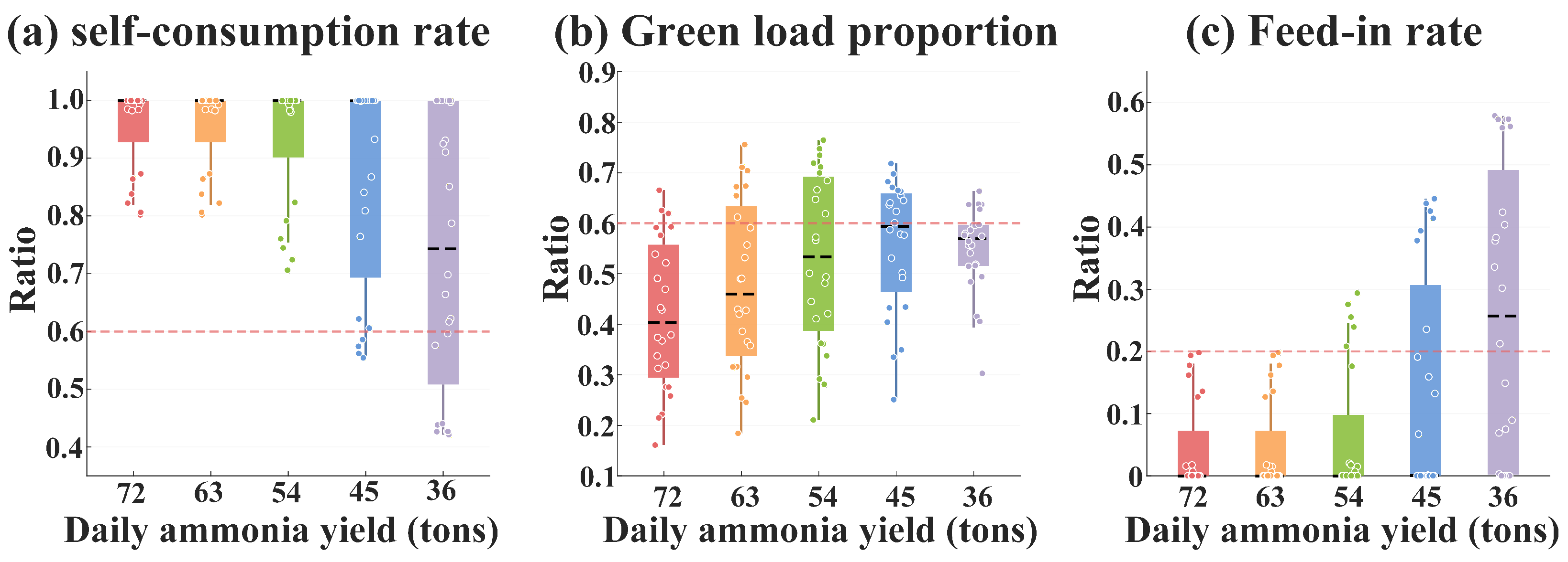
Figure 3 presents the three key renewable energy utilization metrics across five daily ammonia production targets (72–36 tons/day). The self-consumption rate (${\eta }_{\mathrm{RE}}^{\mathrm{self}}$) remains consistently high at approximately 0.94 across all targets, indicating that 94% of available renewable generation is directly consumed by the park regardless of production level. This stability is attributed to the flexible power-to-ammonia conversion chain, which provides a sizable and adjustable electrical load capable of absorbing most renewable output.

The green electricity proportion of total load (${\eta }_{\mathrm{load}}^{\mathrm{green}}$) exhibits a strong inverse relationship with production target, increasing monotonically from approximately 0.64 at 72 tons/day to nearly 0.99 at 36 tons/day. Lower production targets reduce total electrical demand, enabling renewable generation to cover a larger fraction of the scaled-down load. Conversely, the feed-in rate (${\eta }_{\mathrm{RE}}^{\mathrm{grid}}$) decreases as production rises, reflecting reduced surplus renewable generation at higher load levels.

4.1.2. Grid Interaction

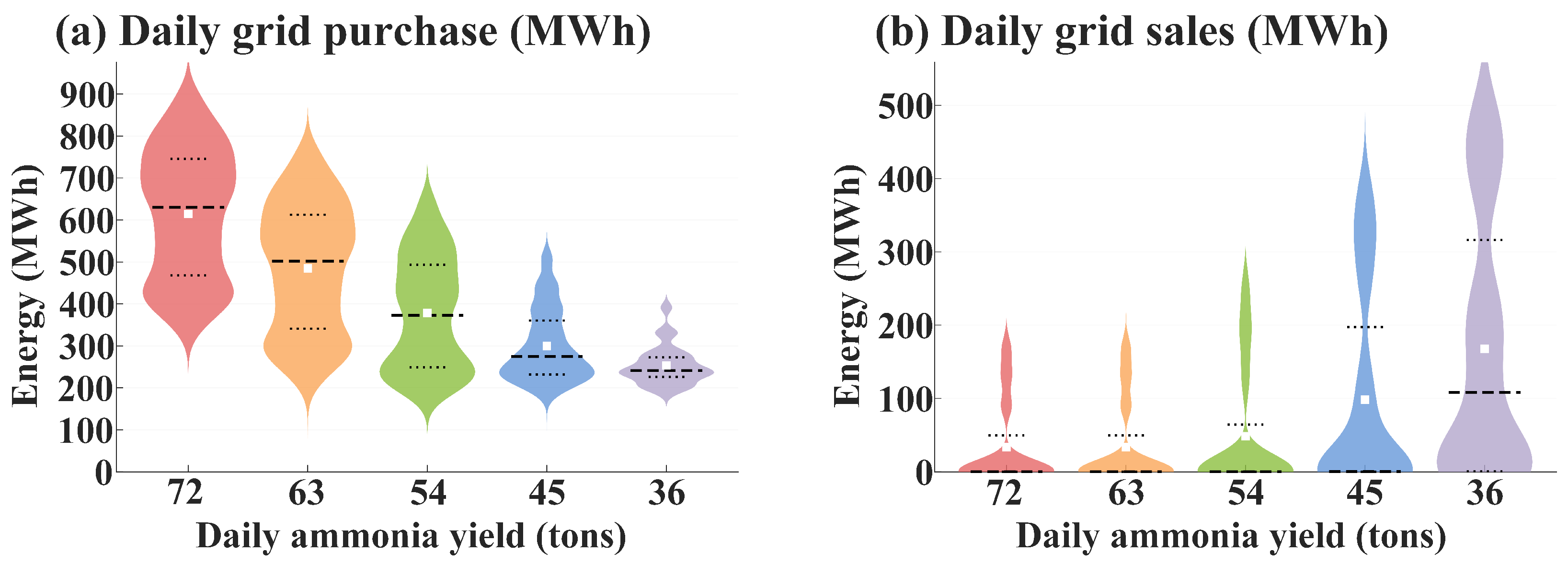
Figure 4 presents violin plots of daily grid purchase and sales across the five production targets. At 72 tons/day, median daily grid purchase is approximately 450 MWh with a wide interquartile range (300–500 MWh), reflecting substantial grid imports required to meet maximum production demand. As the target decreases to 36 tons/day, median grid purchase increases to approximately 720 MWh with reduced variability, indicating that lower production reduces overall load and allows renewable generation to meet a greater share of demand.

Grid sales exhibit the opposite trend. At 72 tons/day, daily sales remain near zero, as the park prioritizes self-consumption for ammonia production. At 36 tons/day, grid sales increase significantly, reaching approximately 200 MWh, reflecting surplus renewable generation that cannot be absorbed by the reduced chemical production.

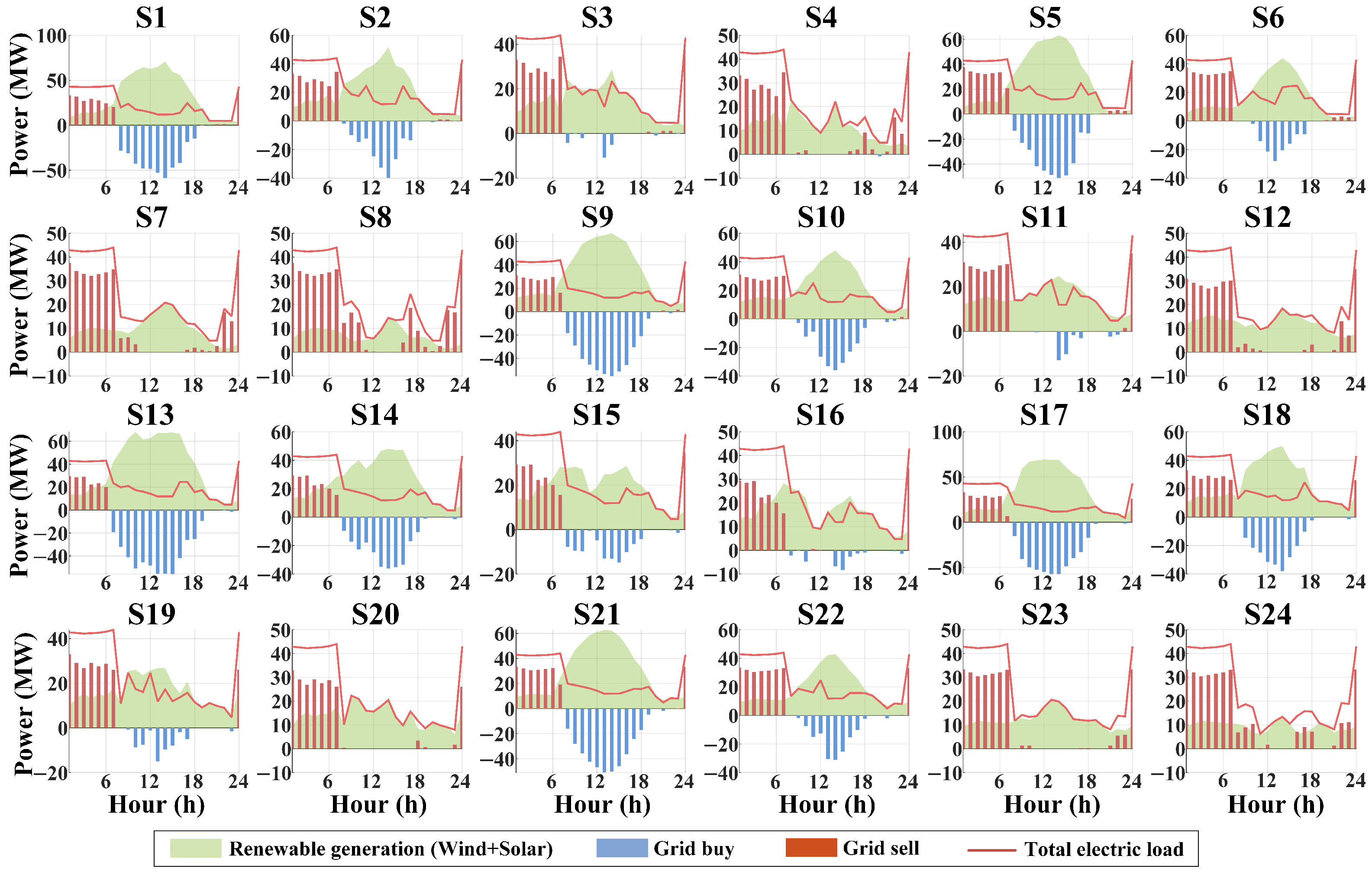
The electrical balance matrix (Figure 5, shown for the 36 tons/day target) confirms that renewable generation dominates supply in all 24 scenarios, with grid purchase compensating deficits during periods of high load or low renewable output. Grid sales occur during renewable surplus periods, particularly when solar generation peaks at midday. The strict mutual exclusivity between purchase and sales at each time step confirms the binary constraints in Equations (3)–(5) are correctly enforced.

4.1.3. Thermal Balance Validation

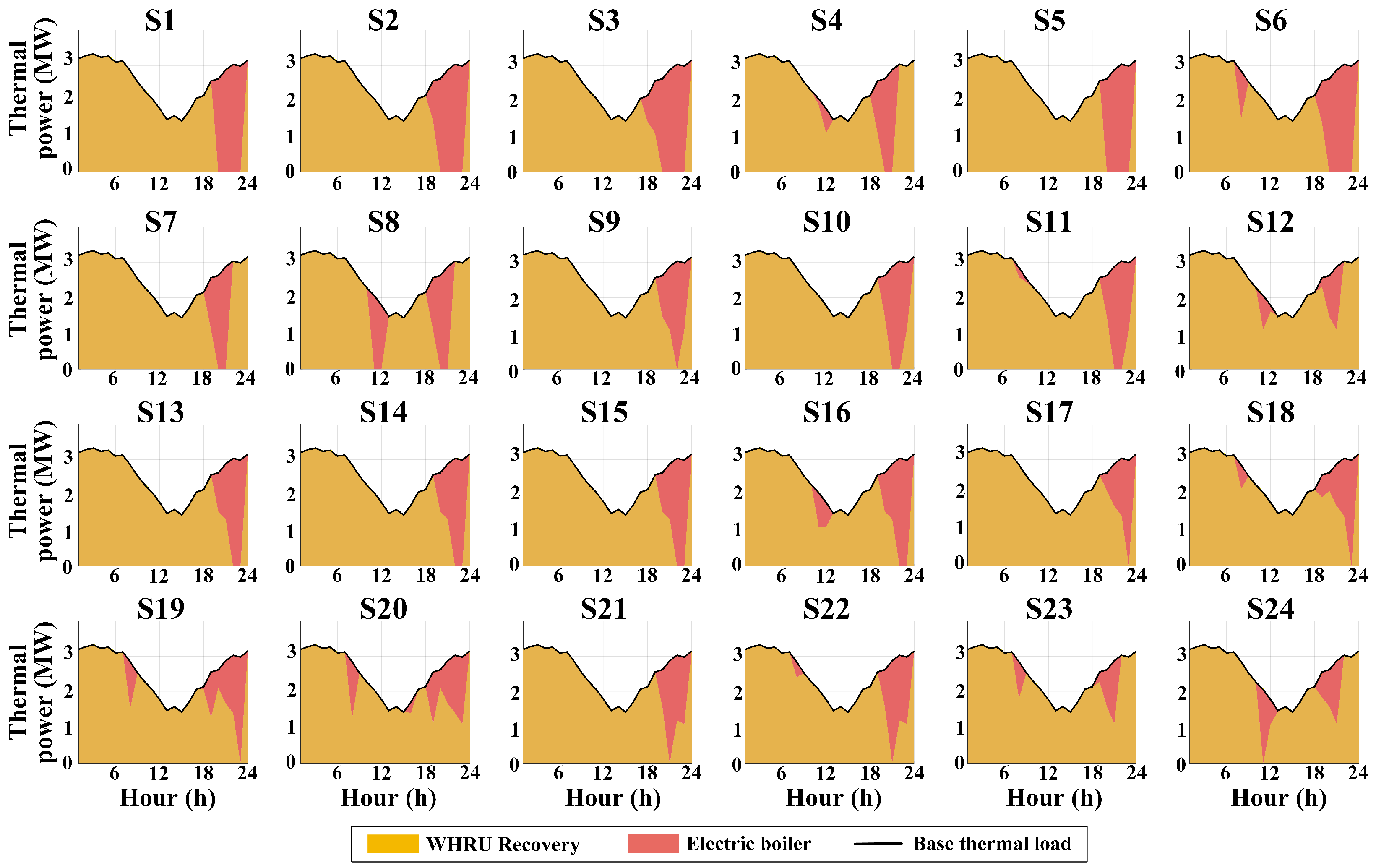
The thermal balance matrix (Figure 6) validates that the base thermal load is consistently met across all scenarios, with WHRU recovery constituting the dominant heat source. EB activation occurs primarily during periods when waste heat from electrolysis and the AMU is insufficient—typically at night or under reduced load conditions. Scenarios with high renewable output exhibit near-complete WHRU coverage, while low-renewable scenarios require substantial EB activation. This confirms the tight electro-thermal coupling inherent to integrated chemical parks.

4.2. Off-Grid Mode Analysis

4.2.1. Dynamic Yield and Economic Performance

In off-grid mode, the system operates without grid support and without a fixed production target, dynamically maximizing ammonia production based on renewable availability.

Table 6. Off-grid optimization results across 24 scenarios.

Group 1			Group 2
Scenario	Yield (tons/Day)	LCOA (RMB/ton)	Scenario	Yield (tons/Day)	LCOA (RMB/ton)
1	47.70	3721.97	13	55.79	3764.47
2	29.25	3860.23	14	38.36	3793.06
3	17.39	4271.11	15	25.96	3986.24
4	12.71	4693.29	16	21.45	4162.41
5	40.70	3687.30	17	51.49	3742.77
6	21.28	4008.65	18	34.40	3795.55
7	9.22	5117.57	19	22.06	4044.03
8	3.68	8508.66	20	17.49	4279.60
9	49.10	3711.53	21	45.01	3675.01
10	31.28	3808.83	22	26.10	3843.32
11	19.31	4117.18	23	14.46	4352.85
12	14.63	4441.49	24	9.06	5201.48

summarizes the optimized yields and levelized cost of ammonia (LCOA) across 24 scenarios. Notably, both curtailment and deficit are zero across all scenarios, confirming that the 195 MWh BESS configuration provides sufficient buffering capacity to absorb all renewable generation and maintain continuous supply under all tested conditions.

Optimized yields range from 3.68 tons/day (Scenario 8) to 55.79 tons/day (Scenario 13), with a median of approximately 22 tons/day. This substantial variation reflects the strong dependence of production capacity on meteorological conditions. LCOA exhibits a strong negative correlation with yield, ranging from 3675 RMB/ton at high yields to 8509 RMB/ton at low yields, underscoring the economic vulnerability of islanded operation during poor renewable resource periods. The median LCOA of approximately 4000 RMB/ton is competitive with reported green ammonia production costs, indicating acceptable economic performance under typical conditions.

4.2.2. Electrical and Thermal Dispatch

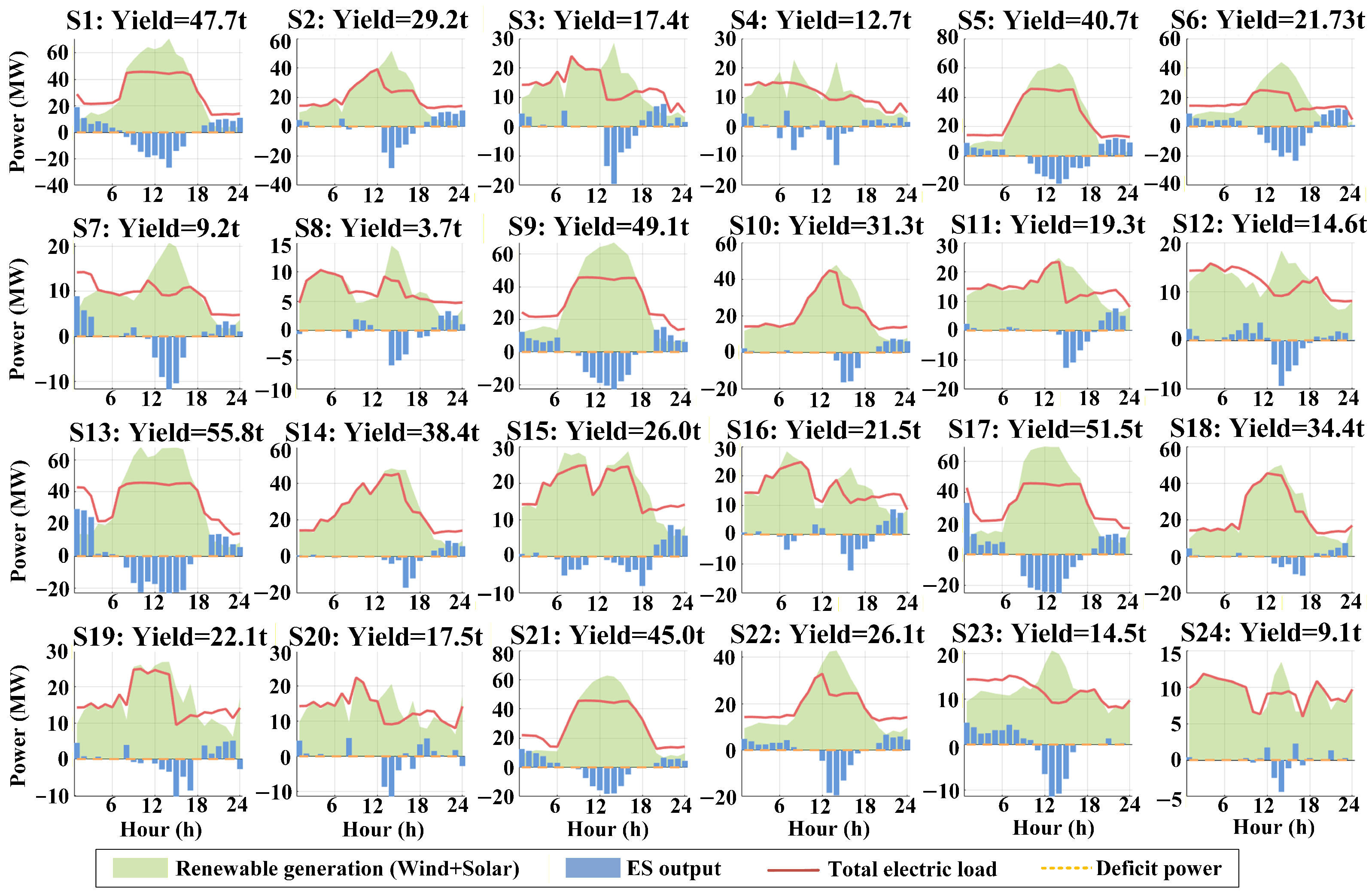
The off-grid electrical dispatch matrix (Figure 7) reveals that renewable generation dominates supply in all scenarios, with BESS serving primarily to bridge temporal mismatches between renewable availability and load demand. BESS charges during midday peak solar periods and discharges during evening and early morning periods when renewable generation is low. The SOC is maintained within 10–90% limits, with initial and final values equal to 60% as required by Equation (28). The total load exhibits clear “source-following-load” behavior, increasing during high renewable periods and decreasing during low-resource periods, demonstrating the inherent flexibility of the power-to-ammonia conversion chain.

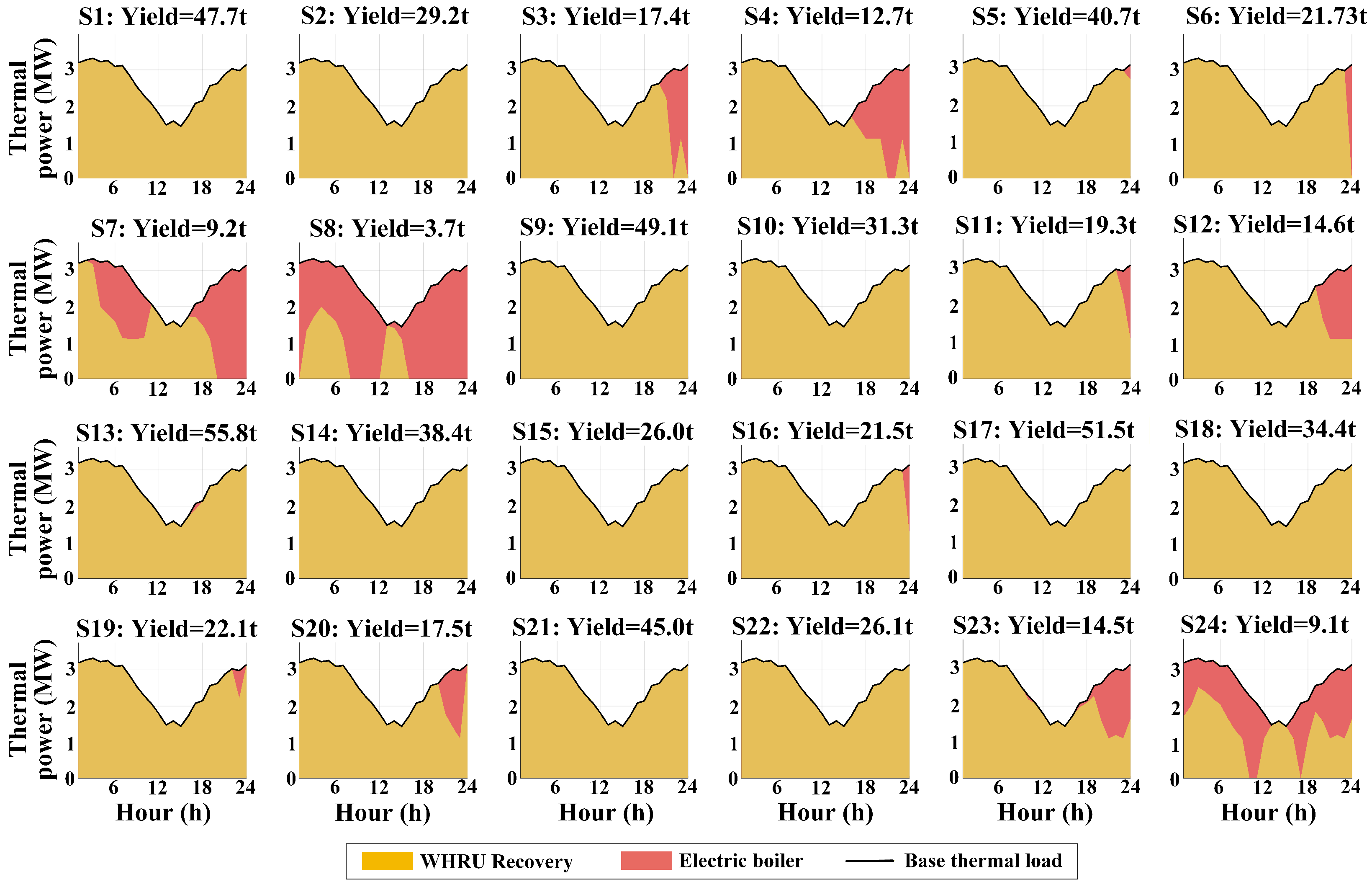
The off-grid thermal balance (Figure 8) confirms consistent thermal load satisfaction across all scenarios. WHRU recovery is generally lower than in grid-connected mode due to reduced and more variable electrolyzer loading under dynamic yield maximization. The EB consequently provides a larger share of thermal demand, particularly during low-renewable scenarios. This highlights the critical role of EB as both a supplementary heat source and a flexible load for power balance maintenance.

4.3. Summary and Physical Consistency

The evaluations presented above confirm that both datasets are physically consistent and thermodynamically feasible. Key validations include: (i) electrical power balance satisfied at every time step; (ii) thermal power balance satisfied with WHRU and EB outputs within physical bounds; (iii) hydrogen mass balance satisfied at every time step; (iv) all equipment operating within 10–100% rated power limits; and (v) BESS SOC maintained within prescribed limits in off-grid operation. No data point violates any physical or operational constraint, ensuring direct applicability to engineering analysis without data filtering.

To provide quantitative evidence of numerical consistency,

Table 7. Quantitative validation of physical constraints across all optimization cases.

Validation Metric	Maximum Residual/Violation
Electrical power balance residual (MW)	<$1\times {10}^{-6}$
Thermal power balance residual (MW)	<$1\times {10}^{-6}$
Hydrogen mass balance residual (kg/h)	<$1\times {10}^{-6}$
BESS SOC constraint violation (%)	<$1\times {10}^{-6}$
Equipment minimum load limit violation (MW)	<$1\times {10}^{-6}$
Equipment maximum load limit violation (MW)	<$1\times {10}^{-6}$
Number of infeasible optimization runs (out of 144)	0

summarizes the constraint validation results across all 144 optimization cases (120 grid-connected cases with 5 yield targets × 24 scenarios, plus 24 off-grid cases). All residual values are within the solver’s numerical tolerance (Gurobi optimality tolerance $=1\times {10}^{-6}$), confirming that the published dataset is numerically reliable and physically rigorous.

These results confirm that all operational states strictly satisfy the physical constraints enumerated in Section 3, with numerical residuals attributable solely to solver tolerance rather than physical inconsistency. The dataset therefore requires no data filtering for engineering applications.

5. User Notes and Applications

5.1. Data Access and Usage Instructions

The complete dataset is publicly available at https://github.com/Data-provider2026/Hourly-Grid-Connected-and-Islanded-Operation-Dataset-for-the-Green-Chemical-Park (accessed on 20 June 2026). All files are provided in CSV format with UTF-8 encoding, ensuring compatibility with major programming environments including MATLAB, Python (3.9), and Microsoft Excel. The dataset is organized into three separate CSV files: the base scenario data, the grid-connected operation records, and the off-grid operation records. Each file follows a consistent naming convention with clear column headers, allowing users to easily extract specific variables for targeted analysis. Users are encouraged to cite this paper when utilizing the dataset in their research. For detailed parameter definitions and model formulations, readers are referred to Section 3 and Appendix A.

5.2. Application Case 1: Capacity Planning and Techno-Economic Assessment

The grid-connected dataset enables capacity planning by allowing users to modify equipment ratings, such as ALKEL capacity or wind-solar installation ratios, and re-run the optimization model to obtain new operational metrics. By comparing levelized costs, renewable penetration rates, and grid interactions across scenarios, optimal configurations can be identified for specific site conditions. The dataset also provides a benchmark for validating simplified planning models against full MILP solutions.

To facilitate future machine learning applications of this dataset, we recommend the following baseline setup for predicting daily ammonia yield in off-grid mode: use 18 scenarios for training and 6 for testing, adopt linear regression and random forest as baseline methods, employ total daily wind and solar generation as input features, and report RMSE, MAE, and $R^2$ as performance metrics. We hope this recommendation provides a useful starting point for researchers interested in applying machine learning to our dataset.

5.3. Application Case 2: Benchmark for Multi-Energy EMS Algorithm Development

The dataset serves as a rigorous benchmark for energy management system (EMS) algorithms. The complete input-output pairs, where renewable availability serves as the input and optimal dispatch as the output, constitute an ideal supervised learning dataset for training neural networks such as LSTM or Transformer models. The 24 scenarios provide diverse conditions for model predictive control (MPC) validation and reinforcement learning agent training. Future EMS algorithms can be benchmarked against the Gurobi-based optimal solutions provided in this dataset.

5.4. Application Case 3: Flexible Production Strategy Validation

The off-grid dataset is suited for studying flexible production strategies under renewable variability. The dynamic yield maximization approach serves as a baseline for developing alternative scheduling policies. Users can modify BESS capacity to explore its sensitivity on system resilience and LCOA, providing insights for storage sizing in islanded chemical parks.

5.5. Limitations and Future Extensions

Several limitations should be acknowledged. First, the data are based on the meteorological characteristics of Jilin, China, and may not directly represent other regions without calibration. Second, the current version adopts steady-state equipment models and does not capture sub-hourly dynamics. Third, the off-grid mode considers only a single BESS capacity (195 MWh). Future extensions will address these limitations by incorporating seasonal variability, multiple BESS configurations, and dynamic equipment models.

We also clarify that the model parameters can be categorized into three types: site-specific parameters (renewable profiles, electricity tariffs) that require recalibration for other locations, generic parameters (electrolyzer efficiencies, operational constraints) that are broadly applicable, and user-adjustable parameters (equipment capacities, economic coefficients, BESS size) that can be customized for different design scenarios.

6. Conclusions

This paper presents a comprehensive, multi-scenario operational dataset for green hydrogen–ammonia parks directly powered by renewable energy. The dataset is constructed upon real-world equipment specifications from a 40 MW wind and 64 MW PV park located in Jilin, Northern China, and spans 24 typical meteorological scenarios that capture the full spectrum of wind-solar variability. Two distinct operational paradigms are systematically addressed: grid-connected mode with five fixed production targets (72, 63, 54, 45, and 36 tons/day) and economic dispatch, and off-grid mode with dynamic yield maximization under a 195 MWh battery energy storage system.

The dataset provides high-resolution (hourly) records of all major energy flows, including renewable generation, electrolyzer and AMU power consumption, grid interaction, BESS state-of-charge, and thermal recovery. All operational states are strictly validated against physical constraints, such as equipment load limits (10–100% rated power), energy conservation laws, thermodynamic recovery bounds (WHRU efficiency of 80%), and BESS SOC limits (10–90%). Quantitative validation confirms that all residuals remain below ${10}^{-6}$ across all 144 optimization cases, with zero infeasible runs.

The novelty of this work lies in three aspects. First, this is the first publicly available dataset that systematically covers both grid-connected and islanded modes for renewable-powered hydrogen–ammonia parks. Second, unlike existing datasets based on statistical or reduced-order models, our data are generated from first-principle physics models with strict enforcement of all physical constraints. Third, the 24 typical meteorological scenarios provide comprehensive coverage of renewable variability, establishing a robust benchmark for EMS algorithm validation. Key performance indicators include a renewable self-consumption rate of approximately 94% across all targets, a green electricity proportion ranging from 64% to 99%, and an off-grid LCOA ranging from 3675 to 8509 RMB/ton with a median of approximately 4000 RMB/ton.

The dataset is publicly available in CSV format. We anticipate that it will serve as a valuable benchmark for capacity planning, EMS algorithm development, flexible production strategy validation, and machine learning-based scheduling studies. By bridging the gap between idealized modeling and practical engineering, this work supports the ongoing transition of high-emission chemical industries toward zero-carbon, flexible, and resilient production systems.

References

- Fortunato, J.; Narciso, C.A.D.; Matos, A.H. Toward the decarbonization of ammonia production through the gradual incorporation of green hydrogen. Ind. Eng. Chem. Res. 2026, 65, 5035–5045. [Google Scholar] [CrossRef] [PubMed]
- Huang, J.; Iglesias, G. Hybrid offshore wind-solar energy farms: A novel approach through retrofitting. Energy Convers. Manag. 2024, 319, 118903. [Google Scholar] [CrossRef]
- Du, W.; Cai, G.; Zhang, J.; Li, Y.; Zhou, Z.; Chen, X.; Nie, S. An integrated spatiotemporal techno-economic assessment of offshore renewable energy complementarity: A case study in China’s maritime zones. Appl. Energy 2026, 410, 127513. [Google Scholar] [CrossRef]
- Zhou, J.; Zhang, Z.; Zhang, R.; Zhang, W.; Xu, G.; Wang, H. Optimal capacity and multi-stable flexible operation strategy of green ammonia systems: Adapting to fluctuations in renewable energy. Energy Convers. Manag. 2024, 314, 118720. [Google Scholar] [CrossRef]
- Liu, Y.; Liu, W.; Liu, J.; Zhang, H.; Li, Z.; Ban, M. Optimal operation strategy for multi-energy systems considering renewable energy fluctuation and carbon emission. Int. J. Electr. Power Energy Syst. 2025, 169, 110794. [Google Scholar] [CrossRef]
- Tang, Y.; Zheng, Z.; Min, F.; Xie, J.; Yang, H. An optimization framework for component sizing and energy management of hybrid electrolyzer systems considering physical characteristics of alkaline electrolyzers and proton exchange membrane electrolyzers. Renew. Energy 2025, 243, 122555. [Google Scholar] [CrossRef]
- Meriläinen, A.; Kosonen, A.; Jokisalo, J.; Kosonen, R.; Kauranen, P.; Ahola, J. Techno-economic evaluation of waste heat recovery from an off-grid alkaline water electrolyzer plant and its application in a district heating network in Finland. Energy 2024, 306, 132181. [Google Scholar] [CrossRef]
- Steinegger, J.; Hammer, A.; Wallner, S.; Kienberger, T. Revolutionizing heat distribution: A method for harnessing industrial waste heat with supra-regional district heating networks. Appl. Energy 2024, 372, 123769. [Google Scholar] [CrossRef]
- Cabral, T.O.; Pourkargar, D.B. Nonlinear predictive regulation of an integrated green hydrogen and ammonia production system under time-varying renewable energy supply. Comput. Chem. Eng. 2026, 204, 109376. [Google Scholar] [CrossRef]
- Banshamlan, M.H.; Mekkawy, E.T.; Sleiti, A.K. Thermoeconomic assessment of a novel multigeneration system for power, hydrogen, ammonia, and methanol production. Int. J. Hydrogen Energy 2026, 237, 155183. [Google Scholar] [CrossRef]
- An, K.; Cai, W.; Lu, X.; Wang, C. High-resolution gridded dataset of China’s offshore wind potential and costs under technical change. Sci. Data 2025, 12, 69. [Google Scholar] [CrossRef] [PubMed]
- Parsa, M.S. Physics-informed machine learning meets renewable energy systems: A review of advances, challenges, guidelines, and future outlooks. Appl. Energy 2025, 402, 126925. [Google Scholar] [CrossRef]
- Kumar, S.; Panagant, N.; Arzaghi, E.; Baalisampang, T.; Garaniya, V.; Abbassi, R. A multi-objective optimisation framework for a standalone hybrid offshore renewable energy system with electrical and hydrogen loads. Energy 2025, 330, 136826. [Google Scholar] [CrossRef]
- Mewafy, A.; Ismael, I.; Kaddah, S.; Sulaiman, A.Y.; Deng, F.; Abulanwar, S. A novel demand response framework for the optimal design of hydrogen-ammonia hybrid microgrids. Appl. Energy 2026, 419, 128074. [Google Scholar] [CrossRef]
Figure 1.
System architecture of the grid-connected green hydrogen–ammonia park. Four energy vectors—electric power, heat power, hydrogen power, and ammonia power—are coordinated through multi-energy conversion and coupling units.
Figure 2.
System architecture of the off-grid green hydrogen–ammonia park with a battery energy storage system (BESS). The islanded configuration eliminates external grid dependency while introducing BESS for renewable variability buffering.
Figure 3.
Renewable energy utilization metrics across five ammonia production targets: self-consumption rate (), green load proportion (), and feed-in rate (). The dashed red line denotes the recommended benchmark for green hydrogen–ammonia parks (e.g., green electricity consumption ratio ). The dashed black lines represent the median values of the corresponding metrics.
Figure 4.
Violin plots of daily grid purchase and grid sales across five ammonia production targets. The dashed lines within the violins represent the median values, while the dotted lines indicate the 25th and 75th percentiles, and the white squares denote the mean values.
Figure 5.
Electrical balance matrix for the grid-connected mode at 36 tons/day target across 24 scenarios.
Figure 6.
Thermal balance matrix for the grid-connected mode at a target of 36 tons/day across 24 scenarios.
Figure 7.
Electrical dispatch matrix for the off-grid mode across 24 scenarios.
Figure 8.
Thermal balance matrix for the off-grid mode across 24 scenarios.