iOrganoAssay to Connect Microscopy Images to Organoid Assays for Long-Term Monitoring

Abstract

We present the use of iOrganoAssay (images of Organoid Assay) to connect microscopy images with organoid assessment assays such as live–dead, immunocytochemistry, and drug treatment assays. The iOrganoAssay consists of an R script-based application (App) interface and datasets encompassing (1) microscopy images, (2) segmentation results, (3) morphometric data, (4) a metadata file, and (5) a validation dataset. The microscopy image collection includes 234 large-area images of intestinal organoids cultured in Matrigel dome region (~3 mm), acquired using an automated stage-equipped microscopy system. Upon treatment with dextran sulfate sodium (DSS), microscopy images of morphological changes in intestinal organoids were captured and quantified. Image segmentation was performed to extract organoid morphological data, including area, perimeter, and circularity. These metrics were plotted to visualize daily variations, enabling systematic tracking of drug-induced morphological changes over time. Statistical comparisons were also provided using violin plots. To evaluate segmentation quality, we established a validation dataset of 28 manually annotated organoids (14 control, 14 DSS-treated) and calculated Dice scores, accuracy (Acc), segmentation error (SegErr), and centroid error (CenErr). This integrated dataset—covering organoid images, segmentation outputs, morphometric data, and validation metrics—provides a resource for organoid image-based studies in morphological monitoring and segmentation validation.

Dataset: The dataset described is publicly available in Zenodo and GitHub. https://doi.org/10.5281/zenodo.18627306 (accessed on 23 May 2026) & https://github.com/swnam153/iOrganoAssay (accessed on 23 May 2026).

Dataset License: CC0

1. Summary

Quantitative imaging-based organoid analysis has attracted significant attention across a broad range of precision medicine and disease modeling applications [1,2,3]. Organoids serve as powerful cellular models that recapitulate the physiological functions of various organs, including the intestine, brain, liver, kidney, lung, and stomach [4]. A particularly important challenge in the organoid research field is the integration of large-scale microscopy image datasets with downstream assay data [5,6,7,8]. Recent advances in artificial intelligence (AI) have opened new opportunities in organoid imaging research, with applications spanning organoid morphology-based phenotyping, patient-derived organoid analysis, and histological scoring [9,10,11,12,13,14]. Organoids have long been valued in drug treatment studies as a key tool for precision medicine [15]. Accordingly, accurate monitoring of organoid growth is essential for toxicology analysis and drug screening. To address these demands, a range of advanced tools, including sophisticated medical devices and microfluidic chips, have been developed to enable efficient, high-throughput screening platforms [16,17,18,19,20,21].

However, efficient data management of organoids based on microscopy images is still a challenge. Organoid morphology is typically categorized into structural forms, including branched (budding), solid, grape-like, and cystic shapes [1,2,3]. Accordingly, the geometrical complexity of organoids influences imaging analysis performance. Notably, the bright-field (BF) images provide fascinating morphological development of organoids, yet automated analysis based on white-black image pixels requires an algorithm to precisely track the complex geometry of organoids. The analysis of large organoid image sets remains labor-intensive and subject to investigator bias, posing challenges for organoid image analysis.

Recently, Schröter, J. et al. reported a brain organoid dataset of 1400 images for 64 trackable brain organoids [22], in which five folds of organoid image sets were analyzed by a cross-validation process for machine learning (ML)-based image segmentation. In the report, CellProfiler [7], OrganoSeg [11], MOrgAna [13], and SegFormer [14] algorithms were tested for the analysis of round shape brain organoids, among which the SegFormer algorithm provides the best scoring in ML-based segmentation of brain organoids. One missing point is that the shapes of brain organoids are relatively simple, having almost circular shapes, thus the tracking of brain organoids is a relatively easy task. It should be tested for the application of more complicated-shaped organoids, such as budding-shaped intestinal organoids [23,24,25].

Another application of AI-based image segmentations is as follows. Histology processing tools such as Indicalab [26] and AIVIA [27,28] have been introduced with embedded AI-based segmentation algorithms, which are designed for general pathological scoring and have been applied to organoid image analysis. Notably, a clinical microscopy dataset of images from urine samples has been reported for the analysis and diagnosis of urinary tract infection by 2D scatter plots of area versus circularity [29], which is meaningful for categorizing cellular morphologies such as epithelial cell sheets, yeast, and blood cells, based on their geometrical features.

Here, we propose iOrganoAssay (images of Organoid Assay), an integrated platform through which 234 organoid images in a large area were analyzed in correlation with downstream assay data, including live–dead assays, immunocytochemistry (ICC), and drug treatment assays [30]. To systematically manage microscopy images alongside assay results, we organized the datasets to encompass raw microscopy images, segmented images, morphometrics data, and images for validations, including the Dice score, accuracy (Acc), segmentation error (SegErr), and centroid error (CenErr). By incorporating a metafile (an Excel spreadsheet file), we established an R script-based application (App) interface capable of visualizing image sets, daily monitoring plots, and statistical analyses. The iOrganoAssay dataset and App interface are designed to support organoid researchers in the integrated management, quantitative analysis, and quality validation of large microscopy datasets, enabling broad accessibility and reuse under a CC0 license.

2. Data Description

2.1. iOrganoAssay Dataset Overview

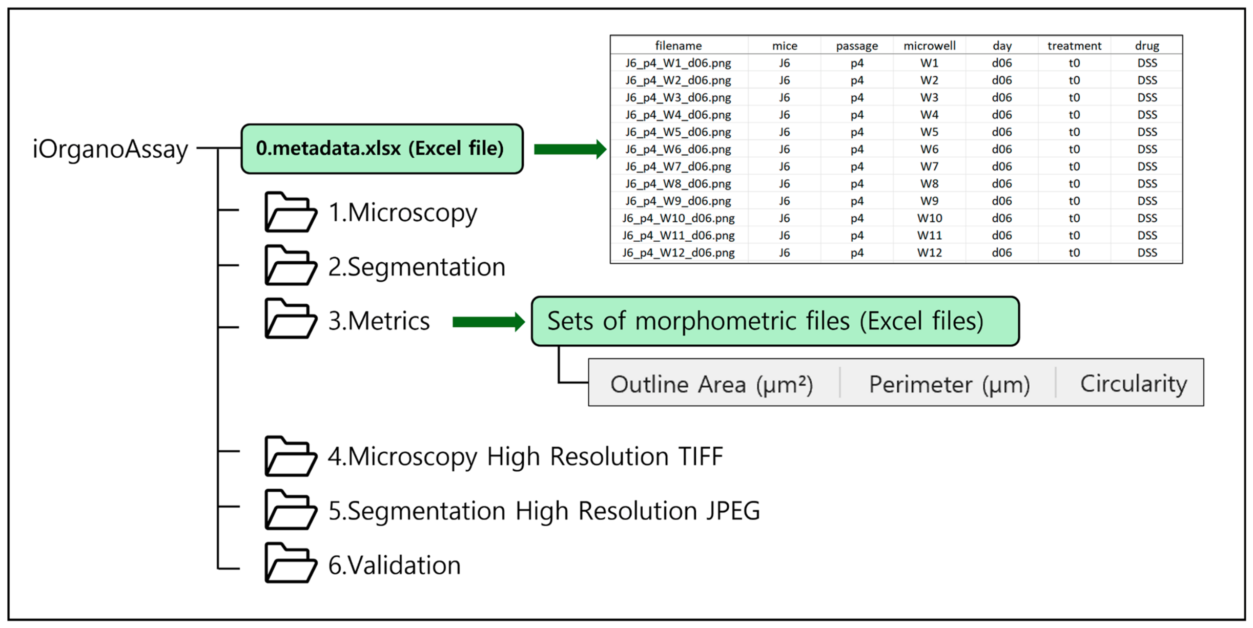
The primary purpose of iOrganoAssay is to connect the microscopy dataset to conventional assays, such as drug treatment and in vitro induction of an intestinal inflammatory model [30], by enabling systematic analysis of mouse intestinal organoid (mIO) morphology under controlled experimental conditions. The dataset is structured by three core subdirectories: 1.Microscopy, 2.Segmentation, and 3.Metrics, unified through a central Excel metafile that cross-references each image file with its corresponding segmentation image and morphometric files (Figure 1). The iOrganoAssay dataset contains 234 microscopy images in total (

Table 1. Microscopy image dataset consisting of 234 images in iOrganoAssay.

Mice	Passage (p)	Microwell (W)	Day (d)	The Number of Images
I6	p1	W1,W2 (2 wells)	d00,d04,d05,d06,d08,d09,d11,d12,d16,d17,d18, d19,d21,d23,d24,d26,d27 (17 days)	34 images
J6	p4	W1,W2,W3,W4,W5,W6,W7,W8, W9,W10,W11,W12 (12 wells)	d00,d03,d06,d09 (4 days)	48 images
N6	p1	W1,W2 (2 wells)	d06,d09 (2 days)	4 images
N6	p4	W1,W2,W3,W4,W5,W6 (6 wells)	d00,d01,d02,d03,d05,d07,d08,d10,d11 (9 days)	54 images
O4	p0	W1,W2,W3,W4,W5,W6 (6 wells)	d00,d03,d04,d05,d07,d11,d12,d14,d18 (9 days)	54 images
O4	p3	W1,W2,W3,W4,W5 (5 wells)	d00,d03,d04,d05,d07,d11,d14,d17 (8 days)	40 images
				Total 234 images

). The metafile records the experimental conditions for each image, such as image file name, mouse line (mice), passage number (p), culture day (d), microwell (W) position, and drug treatment day (t). The Microscopy, Segmentation, and Metrics directories contain raw microscopy images, segmented images, and morphometric files, respectively. In particular, area (μm²), perimeter (μm), and circularity values of individual organoids are listed in the morphometric files.

Throughout the dataset, image filenames follow a structured notation in which each component encodes a specific experimental variable: mouse index (e.g., J6, N6, O4); microWell number (W1–W12), indicating the well position within the 96-well plate; passage number (p0, p1, …), denoting the culture passage; culture day (d00, d01, …, d11), indicating the time point after seeding; and DSS treatment day (t0, t1, t2, t3), corresponding to days elapsed since DSS administration. For example, “J6_p4_W1_d06t0.png” refers to mouse line J6, passage 4, microWell 1, imaged on culture day 6 at the start of DSS treatment (t0).

Three complementary subdirectories are also provided: 4.Microscopy High-Resolution TIFF (~5.1 GB) and 5.Segmentation High-Resolution JPEG, which together supply original high-resolution images, and 6.Validation, which contains the images used to calculate segmentation quality metrics, including Dice score, Acc, SegErr, and CenErr.

2.2. iOrganoAssay Application (App) Interface

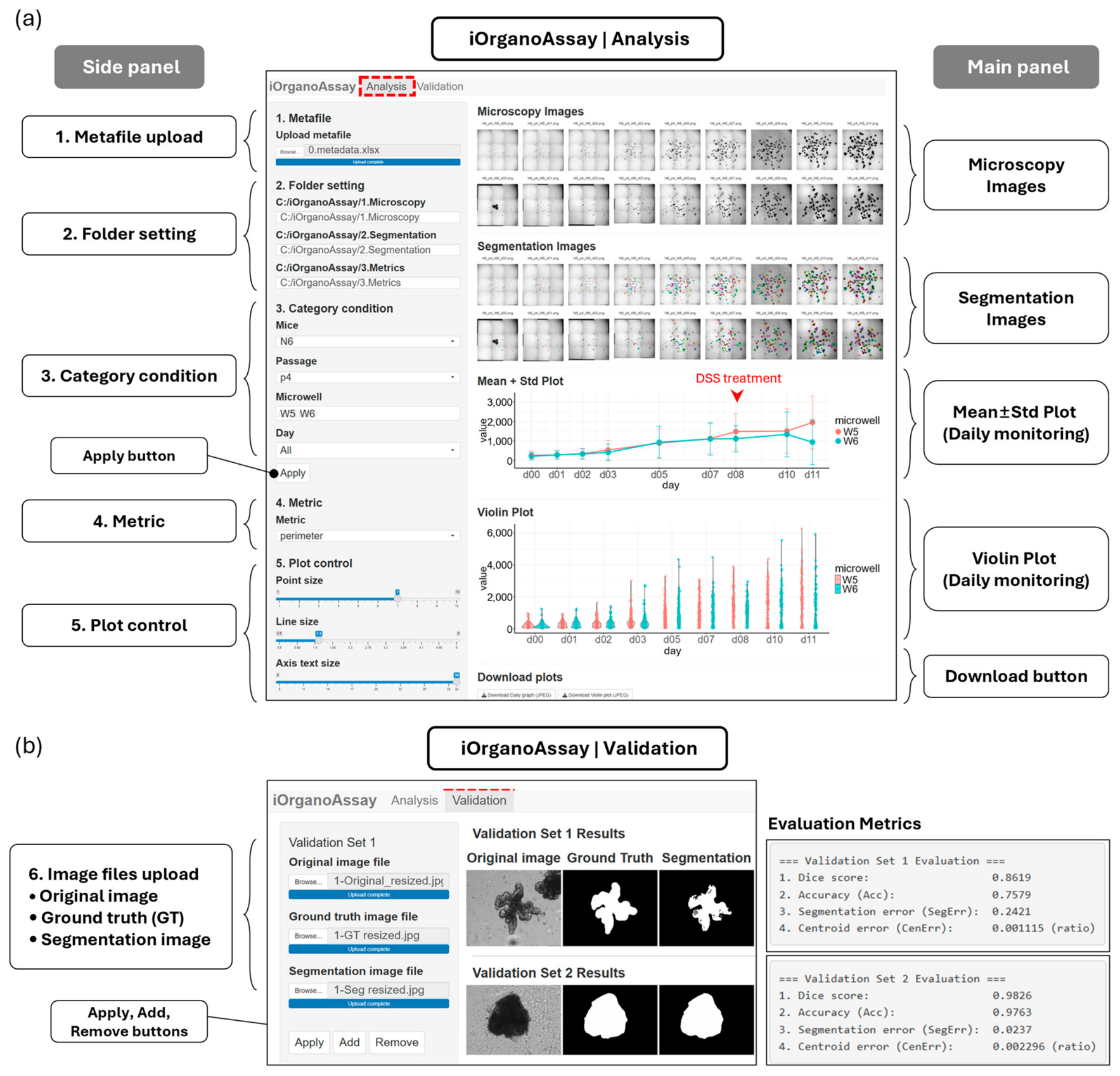
The iOrganoAssay App interface is accessible via a web browser and comprises two tabs in the header: the Analysis tab and the Validation tab (Figure 2). Prior to launching the App, users are required to install the R-based packages by running the installation script available at https://github.com/swnam153/iOrganoAssay (accessed on 23 May 2026), following the instructions provided in the README.md file.

The Analysis tab is divided into a side panel and a main panel (Figure 2a). The side panel integrates five operational modules: (1) metafile upload, in which the metadata Excel file (C:/iOrganoAssay/0.metadata.xlsx) is loaded; (2) folder setting, in which local directory paths for the Microscopy, Segmentation, and Metrics folders are specified; (3) category condition, in which images are filtered by mouse line (Mice), passage (p), microwell (W), and culture day (d), followed by clicking the “Apply” button; (4) metric selection, in which one morphological metric—area, perimeter, or circularity—is chosen for visualization; and (5) plot control, in which visualization parameters including point size, line size, and axis text size are adjusted. The main panel displays microscopy images and segmentation images that satisfy the selected conditions, along with mean ± standard deviation (SD) line plots and violin plots of the chosen metric across culture days. Completed plots can be downloaded as JPEG files via the Download button. For practice, the required dataset—comprising the metafile (0.metafile.xlsx) and three data folders (1.Microscopy, 2.Segmentation, and 3.Metrics)—is provided in the Zenodo repository at https://doi.org/10.5281/zenodo.18627306 and can be downloaded and placed in the desired local directory.

The Validation tab provides a dedicated interface for quantitative evaluation of segmentation quality (Figure 2b). In the side panel, users upload three image files per validation set: an original microscopy image, a ground truth (GT) image, and a segmentation image. Multiple validation sets can be managed using the Apply, Add, and Remove buttons. The main panel displays the original image, ground truth image, and segmentation image side by side, together with four evaluation metrics: Dice score, Acc, SegErr, and CenErr. The image files required for validation are provided in the 6.Validation folder of the Zenodo repository at https://doi.org/10.5281/zenodo.18627306.

3. Methods

3.1. Automation of Microscopy Imaging of Drug-Treated Organoids

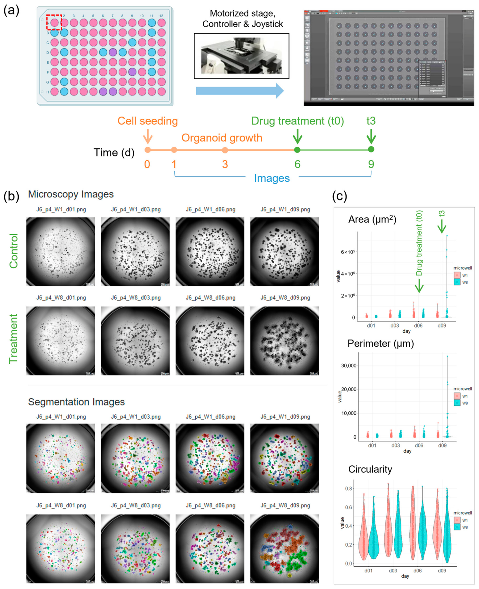
The automated microscopy imaging for the dataset is illustrated in Figure 3. The purpose of our iOrganoAssay dataset is efficient daily management of organoid growth. For this, automated-stage microscopy was used to monitor organoid growth (Figure 3a). We obtained large-area images covering the Matrigel dome region, such as a 3 × 3 mm area within a 6.8 × 6.8 mm 96-microwell (red dotted box in Figure 3a). In a single Matrigel dome, at least several tens of intestinal organoids were grown as the seeding cell density was ~5 × 10⁵ #/mL. Both microscopy and segmented images are displayed (Figure 3b). Additionally, variations in morphological metrics are presented with and without DSS treatment (Figure 3c). BF large area images were taken with a 5× objective lens and transmitted light BF illumination.

The timing of DSS treatment was determined on the basis of the growth status of the organoids. Conventionally, organoid growth depends on the seeding density. Although our culturing protocol does not perfectly control seeding density, it consistently allows DSS treatment to be initiated between d06 and d08, with an additional 3–4 days of culturing thereafter. DSS was administered by addition to the culture medium with a 0.04 mg/mL concentration.

3.2. Image Segmentation Analysis of DSS-Induced Morphological Changes in Organoids

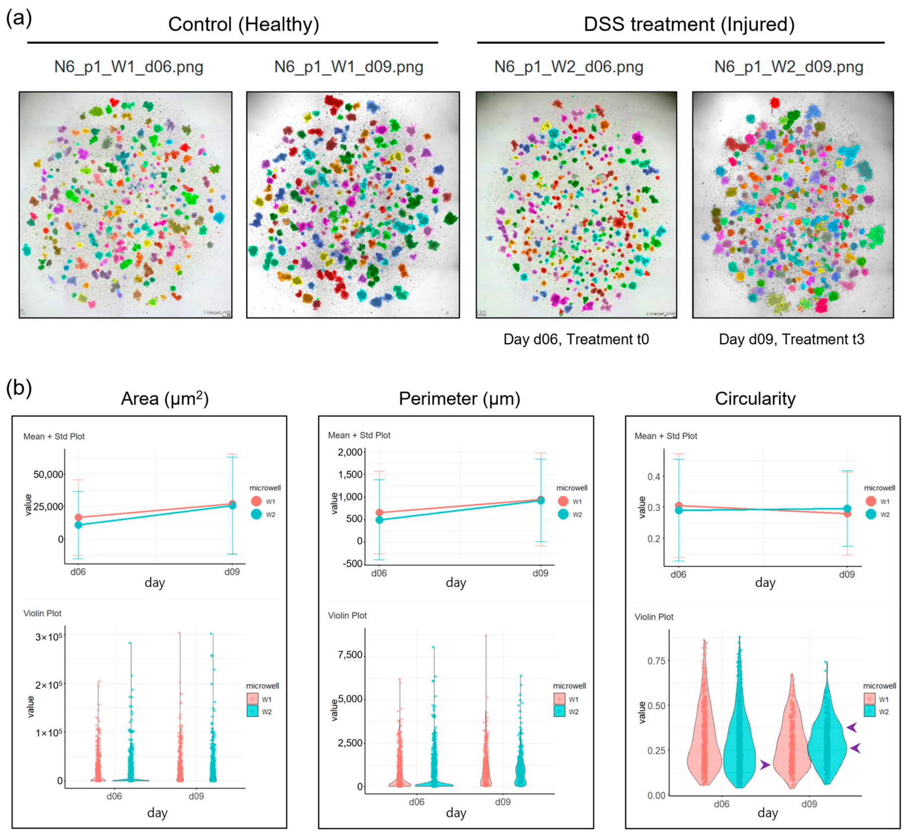
Quantitative differences between control and DSS-treated organoids are further illustrated (Figure 4). Segmentation images from days d06t0 (treatment day 0) and d09t3 (treatment day 3) are shown for control microwell W1 and DSS-treated microwell W2 (Figure 4a). Both groups exhibited increasing area and perimeter values from d06t0 to d09t3, reflecting overall organoid growth over time (Figure 4b). However, no clear difference in area or perimeter was observed between the control and DSS-treated organoids at d09t3. In contrast, circularity showed a notable difference between the two groups at d09t3. Although the Mean ± Std plots revealed no clear separation between W1 and W2, the violin plots provided a more informative view: the circularity distribution in DSS-treated organoids (W2) at d09t3 shifted toward higher values, with broadening in the upper region of the violin, as indicated by purple arrows in Figure 4b. This broadening indicates that a substantial proportion of DSS-treated organoids shifted toward rounder, more circular shapes—a direct consequence of epithelial disruption caused by DSS treatment. This subtle yet consistent shift in circularity distribution, not captured by mean-based summary statistics alone, underscores the value of violin plots for detecting morphological changes in organoid populations.

For large-scale image segmentation, AIVIA (version 15, Leica Microsystems, Wetzlar, Germany) classifier-based segmentation was employed, as described in our previous report [30]. In AIVIA, the classifier is a machine learning-based pixel classifier that assigns each pixel to either the “organoid” (target) class or the “background” class. Raw BF images acquired on the Leica DMi8 system were imported into AIVIA directly from the native LIF format produced by LAS-X, without additional preprocessing such as contrast adjustment or denoising, because the automated-stage acquisition ensured uniform illumination across the Matrigel dome region. Briefly, organoid bodies and background regions in representative images were manually annotated as separate classes, with background regions broadly annotated over non-target areas to enhance classifier discrimination, and the classifier was trained on these annotations. Regarding the specific settings for the organoid target class, the output mode was switched from confidence mode to segmentation mode, whereas the background class remained in confidence mode. In segmentation mode, a binary organoid mask was generated for downstream measurement. After applying the trained classifier across the full image set, segmentation results were continuously inspected via visual verification; if non-target regions were incorrectly classified as target objects, supplementary annotations were provided, and the classifier was iteratively retrained until satisfactory segmentation performance was achieved. Any clearly mis-segmented objects were corrected manually within AIVIA. Per-organoid morphometric outputs (area, perimeter, circularity) were then exported as scatter plots and spreadsheets.

These per-organoid measurements constitute the quantitative output of the iOrganoAssay dataset and support downstream statistical comparison, model validation, and tracking of organoid status.

3.3. Validation for the Image Segmentation of the Organoids

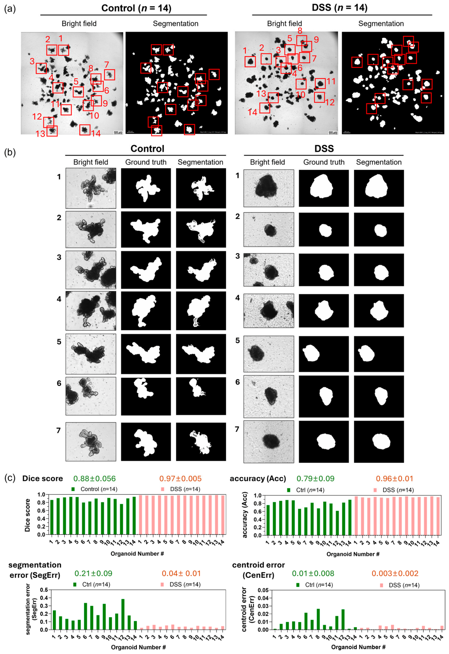
To evaluate the performance of the AIVIA software image segmentation, we established a validation platform using ground-truth (GT) images and segmentation images of the control group and DSS-treated group. Two large-scale bright-field images, acquired with a 5× objective lens [30], were processed with the AIVIA software to obtain the corresponding segmentation images (Figure 5a). One image set was from the control group (mice N6, passage p4, microwell W1, day d08, no treatment), and the other was from the DSS-treated group (mice N6, passage p4, microwell W2, day d08, treatment t1). From each large-area image, 14 organoids were selected and marked with red boxes (numbered 1–14) for ground-truth annotation and AIVIA classifier-based segmentation, of which seven representative organoids per group are displayed (Figure 5b). The remaining seven organoids per group were used only for the quantitative metric calculations (Figure 5c).

Four metrics were calculated to quantify segmentation performance: Dice score, Acc, SegErr, and CenErr. The Dice score measures the spatial overlap between the predicted segmentation (P) and the ground truth (G), defined as Dice = 2|P ∩ G|/(|P| + |G|), with values closer to 1 indicating better overlap. Acc is defined as the proportion of correctly classified pixels (true positives plus true negatives) over the total pixels within the analysis region. SegErr is defined as the normalized area difference, SegErr = ||P| − |G||/|G|, capturing the relative deviation in segmented area. CenErr is defined as the Euclidean distance between the centroids of P and G, normalized by the image diagonal, reflecting positional accuracy.

For each metric, the mean ± standard deviation was calculated separately for the control and DSS-treated groups and is presented in Figure 5c. Across all four metrics, the DSS-treated group shows consistently high segmentation quality with low inter-organoid variability, while the control group exhibits lower scores and larger variation among individual organoids.

We attribute this difference to the effect of DSS treatment, which disrupts the budding epithelial architecture of intestinal organoids and produces more rounded morphologies. Control organoids, in contrast, retain complex protruding budding structures (Figure 5b, control #1–#7). We therefore report both groups transparently rather than presenting only the best-performing subset, so that the iOrganoAssay dataset can serve as a useful benchmark for developing improved segmentation methods targeting morphologically complex, budding-shaped organoids.

4. User Notes

4.1. How to Use the iOrganoAssay App Interface

(1) (optional) Download and install the latest version of RStudio (https://posit.co/download/rstudio-desktop/ (accessed on 23 May 2026))

(2) Download th iOrganoAssay dataset at https://doi.org/10.5281/zenodo.18627306 (accessed on 23 May 2026)

(3) Install the required R packages from https://github.com/swnam153/iOrganoAssay (accessed on 23 May 2026), and launch the iOrganoAssay App in RStudio, following the instructions in README.md and Section 4.2.

4.2. Path of Directories: Microscopy, Segmentation, and Metrics

(1) As noted in Figure 1, the three folders (1. Microscopy, 2. Segmentation, and 3. Metrics) should be located in the same folder as the metadata file (an Excel file).

Default folders are as follows:

• C:/iOrganoAssay/1.Microscopy
• C:/iOrganoAssay/2.Segmentation
• C:/iOrganoAssay/3.Metrics

The default location of the metadata is as follows:

• C:/iOrganoAssay/0.metadata.xlsx

(2) Install the R-based packages by running the installation script.

• # install.packages(“remotes”) # if not already installed
• remotes::install_github(“swnam153/iOrganoAssay”)
• remotes::install_github(“swnam153/iOrganoAssay”, force = TRUE)

(3) Launch the iOrganoAssay App interface.

• library(iOrganoAssay)
• LaunchApp()

(4) Set the metadata file (Excel file) location in the left panel of the App interface. Additionally, the paths of the three folders should be manually edited in the left panel.

(5) Click the “apply” button in the left panel of the App interface.

(6) After confirming the list of images, segmented images, and graphs, adjust the category conditions such as mice, passage (p), microwell (W), and day (d), before repeated clicking of the “apply” button. When you leave the conditions set to “all”, all the images that satisfy the other category conditions are displayed, and you can then sort the images of your interest by selecting specific category conditions.

(7) Adjust metrics such as organoid area, perimeter, and circularity.

(8) Adjust the graph displaying conditions such as dot size, line size, text size, and title size of the graph plot and violin plot.

4.3. Data Dictionary

The dataset (5.3 GB total) consists of

• 0.metadata (Excel file)
• 1.Microscopy images (234 PNG files)
• 2.Segmentation images (234 PNG files)
• 3.Metrics (234 Excel files)
• 4.Microscopy High Resolution (234 TIFF files, 5.1 GB)
• 5.Segmentation High Resolution (234 JPEG files)
• 6.Validation images (2 folders, 14 JPEG files per folder)

To facilitate seamless data integration and ensure reproducibility, users can easily customize the data input by modifying the provided templates (such as 0.metadata.xlsx and the spreadsheets in the 3.Metrics folder), provided that the original header and tab structures are maintained. The column information of 0.metadata.xlsx is listed in

Table 2. Metadata file, column information.

Column	Description	Example
Filename	Image file name	J6_p4_W1_d06.png
Mice	Mouse line ID	J6, N6, O4
Passage	Subculture passage number	p1, p4
Microwell	Microwell position	W1–W12
Day	Culture day	d00, d06
Treatment	Treatment day relative to drug addition	t0, t3
Drug	Drug used	DSS, none

.

Each of the 234 Metrics files (Excel format) in 3.Metrics folder contains the following sheets:

• Summary
• Outline Area (µm²)
• Perimeter (µm)
• Circularity
• Mean Intensity

4.4. Limitations

Image segmentation of organoid microscopy data has been approached using various tools, including ImageJ [5,6], CellProfiler [7], EBImage [8], OrganoSeg [11], and MOrgAna [13]. However, accurately delineating complex organoid morphologies remains technically challenging, and large-scale datasets often still require substantial manual correction. Recently, ML-based methods such as SegFormer [14,22] have been applied to organoid detection, though these represent general-purpose segmentation frameworks not specifically tailored for organoid analysis.

Our iOrganoAssay platform, described here, addresses this challenge by providing a structured workflow capable of managing several hundred microscopy images, enabling integrated visualization of images and quantitative metrics within a single App interface.

In terms of dataset size, the current iOrganoAssay dataset comprises 234 images, which is smaller in image count compared to previously reported datasets such as the brain organoid dataset of 1400 images [22]. However, each image in iOrganoAssay covers a large field of view (~3 × 3 mm Matrigel dome region), capturing tens to approximately 100 individual intestinal organoids per image. Accordingly, the per-image organoid yield is substantially higher, and the dataset as a whole encompasses a broad range of morphological variation across multiple experimental conditions, mouse lines, passages, and drug treatment time points.

The generalizability of the iOrganoAssay dataset and segmentation workflow to other experimental settings should also be considered. The present dataset was acquired exclusively from mouse intestinal organoids cultured under defined Matrigel-dome conditions, and all images were captured on a single Leica DMi8 widefield system at a fixed magnification and illumination setting. Application of the same workflow to organoids derived from other organs (e.g., brain, liver, lung), to alternative imaging platforms (e.g., confocal, light-sheet, or other bright-field systems), or to images acquired under different magnifications and illumination conditions will likely require classifier retraining within AIVIA and additional benchmarking to confirm reproducibility of the morphometric outputs. The iOrganoAssay platform itself, including its directory structure, metafile schema, and R-based App interface, is designed to remain applicable across such extensions, so that new datasets generated under different conditions can be integrated and analyzed within the same framework.

5. Conclusions

Organoid geometry, which reflects the physiology of the original organ, spans a wide range of shapes—including budding, grape-like, solid, and cystic (hollow bloom-like) morphologies—and the shape itself can serve as a morphological readout. In the iOrganoAssay dataset, we focused on the validation of image segmentation for intact and injured intestinal organoids, which present distinct geometrical complexities. Intact intestinal organoids exhibit a budding (branched) geometry originating from the crypt–villus intestinal folding structure, while injured intestinal organoids adopt a rounded shape due to disruption of the epithelium. Notably, segmentation of the budding shape yielded a lower Dice score and Acc due to its geometric complexity, whereas segmentation of the injured organoids yielded a higher Dice score and Acc due to their relatively simple round shape. This dependence of validation scores on geometrical complexity—complex branched versus simple round shapes—represents a novel aspect of the iOrganoAssay dataset. Whereas previously reported organoid image datasets have largely focused on morphologically simple, round-shape organoids such as brain organoids [22], iOrganoAssay provides a benchmark of intestinal organoids spanning both complex branched and simple round geometries within a single dataset. We anticipate that this resource will support the development and validation of next-generation segmentation algorithms for morphologically complex organoids.

Regarding segmentation quality, the iOrganoAssay platform incorporates a validation framework (Section 3.3) in which segmentation performance is assessed using standard metrics, including Dice score, Acc, SegErr, and CenErr. These metrics are accessible directly through the App interface, enabling users to evaluate segmentation reliability.