A Decadal Dataset of Offshore Weather and Normalized Wind–Solar Power Yield for Long-Term Evolution and Capacity Siting Planning in the Beibu Gulf, China

Abstract

For offshore renewable energy planning and intelligent power management, access to long-term, high-resolution, and physically consistent meteorological and power generation records is essential. Such data supports a wide range of tasks, including resource assessment, hybrid system capacity sizing, grid operation planning, and data-driven forecasting model development. This article presents the construction of a 10-year continuous hourly dataset for 16 deep-sea grid sites in the Beibu Gulf, China, spanning from January 2016 to December 2025. The raw meteorological variables, including 10 m wind speed, wind direction, solar irradiance, and 2 m air temperature, were retrieved from the NASA POWER satellite database and subsequently cleaned using a 24 h periodic substitution algorithm designed to preserve the physical integrity of daily weather cycles. The dataset is organized into two sub-datasets, the Historical Weather Dataset and the Normalized Power Yield Dataset, with the latter providing normalized wind and solar power outputs on a 1.0 per-unit (p.u.) basis derived from a wind turbine power curve model and a PV thermodynamic model. All 32 CSV files are freely accessible online with UTF-8 encoding. The utility of the dataset is illustrated through two representative application cases including offshore site selection with hybrid capacity sizing and physics-informed deep learning forecasting, demonstrating its suitability for both engineering analysis and machine learning model development.

Dataset: https://github.com/Lee-ziniu/10-Year-Hourly-Offshore-Weather-and-Wind-Solar-Power-Dataset-for-the-Beibu-Gulf.git (accessed on 1 April 2026).

Dataset License: CC–BY Attribution 4.0 International

1. Introduction

The global shift toward low-carbon energy systems has driven the rapid growth of renewable energy technologies, particularly wind and solar power [1,2,3]. As key parts of future clean energy systems, these resources play an important role in cutting greenhouse gas emissions and addressing climate change. However, their variable and unpredictable nature creates serious challenges for power system management, grid stability, and energy market operations [4,5,6].

Among all renewable options, offshore areas have become highly attractive for energy development due to their stronger and steadier wind conditions, lower surface friction, and more stable weather compared to land-based sites. These features make offshore regions more suitable for large-scale power generation [7,8]. At the same time, offshore solar photovoltaic (PV) systems have attracted growing interest, especially floating PV installations, because they can use the ocean surface without taking up land space [9,10,11]. Combining wind and solar resources in hybrid systems has been widely recognized as a practical way to reduce output fluctuations, since the two sources naturally match each other across both daily and seasonal cycles [1,12,13,14].

Despite these advantages, a key gap in offshore renewable energy research is the shortage of long-term, detailed, and location-consistent datasets that cover both weather conditions and the corresponding power outputs at the same time. Existing global datasets such as ERA5 provide useful large-scale weather information but are often limited by low spatial detail and location-specific errors, especially in coastal and deep-sea areas [15,16]. In addition, most publicly available datasets focus on either wind or solar resources alone and do not include combined representations of hybrid energy systems. In particular, existing offshore datasets [17,18] predominantly emphasize wind resources, with limited attention to offshore solar PV. However, with the rapid advancement of floating PV technology, offshore solar is becoming increasingly feasible and should no longer be overlooked. This limits their usefulness for multi-source system modeling, hybrid capacity planning, and long-term output analysis [19,20]. To state the distinction compactly, unlike reanalysis-based products (e.g., ERA5) or wind-only offshore datasets, the present work provides an open-access, 10-year hourly compilation that concurrently delivers raw meteorological variables and physically normalized wind–solar power outputs for 16 deep-sea grid sites, enabling hybrid planning and forecasting tasks that cannot be adequately supported by existing alternatives.

Beyond data availability, converting weather variables into power output adds further difficulty. Purely data-driven methods, while increasingly common, often lack clear physical meaning and may break the physical operating limits of energy equipment. On the other hand, purely physics-based models need detailed settings and may not capture complex time-varying patterns well. Recent research has therefore focused on combining data-driven and physics-based methods, using advances in machine learning and deep learning [16,21,22,23]. Models such as Long Short-Term Memory (LSTM) networks have shown strong ability to learn time-dependent patterns in renewable energy data, while tree-based ensemble methods such as gradient boosting offer strong nonlinear modeling performance. However, the quality of these methods depends heavily on access to high-quality datasets with enough time coverage, spatial range, and physical accuracy.

To address these gaps, this paper presents a 10-year (2016–2025) continuous hourly dataset for 16 deep-sea grid sites in the Beibu Gulf, China. The dataset combines satellite-based weather data with physics-based power conversion models to produce both raw weather records and normalized power outputs for wind and solar generation. Using a per-unit (p.u.) format ensures that results are easy to compare across different equipment types and can be scaled to any installed capacity. A key feature of this dataset is its use of step-by-step physical models, including wind speed height correction, turbine power curve calculation, and PV cell temperature modeling. These steps keep all power output values within realistic physical operating limits, connecting raw weather data directly to practical engineering use. Beyond the dataset itself, two practical application cases are included to demonstrate its value: one covering offshore site selection and hybrid capacity sizing, and one demonstrating physics-informed deep learning forecasting at multiple time scales. These cases are presented as illustrative demonstrations of how the dataset can be used, rather than as full validations of any specific method or design conclusion.

The main contributions of this work can be summarized as follows:

• Development of a 10-year continuous hourly offshore dataset covering 16 deep-sea grid sites in the Beibu Gulf;
• Integration of meteorological variables and physics-based normalized power outputs within a unified data framework;
• Implementation of physically consistent modeling methods to ensure realistic and bounded power generation;
• Demonstration of dataset applicability in hybrid system planning and physics-informed deep learning forecasting.

Overall, this dataset provides a robust and scalable foundation for offshore renewable energy research, enabling both engineering-oriented analysis and advanced data-driven modeling. It is expected to support future studies in hybrid energy systems, renewable resource assessment, and intelligent forecasting, thereby contributing to the ongoing transition toward sustainable energy systems.

2. Data Description

This dataset provides a vast and detailed collection of historical weather conditions and renewable power generation data for 16 deep-sea grid sites in the Beibu Gulf, China. The data spans a continuous timeframe from 1 January 2016 to 31 December 2025. This 10-year period is helpful for understanding long-term climate variations and ocean weather patterns. Instead of providing broad daily averages, the dataset maintains a strict hourly time resolution. This high frequency results in exactly 87,672 h of observation data for each of the 16 locations. When combining all the spatial grids together, the complete dataset reaches a total of 1,402,752 data rows.

A common challenge with such a large volume of data is that many standard software programs cannot process it easily. For example, Microsoft Excel has a strict limit of one million rows, which would cause the software to crash when opening this 1.4-million-row database. To solve this problem and ensure the data is highly accessible for all users, the massive dataset is structurally decoupled into two separate sub-datasets. All the information is systematically archived in CSV format. The UTF-8 encoding was utilized so that the files can be processed safely on any operating system, such as Windows, macOS, or Linux.

2.1. Historical Weather Dataset

The first sub-dataset focuses entirely on the weather conditions. This folder is named Historical Weather Dataset. Inside this directory, there are 16 separate CSV files. One specific file is dedicated to each ocean grid site to keep the spatial data properly organized. Every file is structured with exactly 12 columns. The detailed explanations of these 12 weather and location variables are as follows:

• SITE: This is the textual identifier assigned to each location. They are numbered simply from S1 to S16. By using these short names, users can easily select one specific site to study without typing long coordinate numbers.
• LON (Longitude): This represents the longitude position of the site on the map, measured in decimal degrees East. Longitude is necessary to know the exact distance of the grid from the coastline.
• LAT (Latitude): This represents the latitude position of the site, measured in decimal degrees North. Together with the longitude, it helps find the exact deep-sea location.
• YEAR: This column shows the calendar year of the weather data. The data goes continuously from the start of 2016 to the end of 2025.
• SE (Season): This column divides the year into four weather seasons. We use the number 1 to represent Spring (from March to May). The number 2 represents Summer (from June to August). The number 3 represents Autumn (from September to November). Finally, the number 4 represents Winter (from December to February).
• MO (Month): This is the month of the year, shown by numbers from 1 (January) to 12 (December).
• DY (Day): This shows the specific day of the month. The dataset includes the correct number of days for different months, as well as the extra day in leap years.
• HR (Hour): This represents the exact hour of the day when the data was recorded. We use the standard 24 h UTC format. The values start at 0 (midnight) and end at 23 (11:00 PM).
• WS10M (Wind Speed): This is the wind speed measured at a standard height of 10 m above the sea surface. The unit is meters per second (m/s). This is a basic and very important variable because it is used directly to calculate the wind power that a turbine can produce.
• WD10M (Wind Direction): This shows the direction from which the wind is blowing. The values range from 0° to 360°. Knowing the wind direction is highly important for engineers when they design the layout of an offshore wind farm, helping them avoid energy losses caused by turbines blocking each other.
• SI (Solar Irradiance): This represents the direct sunlight that reaches the ocean surface, measured in Watts per square meter (W/m²). This variable gives the basic energy input needed to calculate the electricity production of solar panels.
• T2M (Ambient Temperature): This is the air temperature, representing conditions at a height of 2 m. The unit is degrees Celsius (°C). This temperature is critical because when the environment is extremely hot, solar panels suffer from heat loss. They lose their efficiency and produce less power.

To provide a clear understanding of how these 12 variables are structured,

Table 1. Example data in the Historical Weather Dataset (Sample from Grid S1).

SITE	LON (°)	LAT (°)	YEAR	SE	MO	DY	HR	WS10M (m/s)	WD10M (°)	SI (W/m2)	T2M (°C)
S1	108.45	20.10	2016	4	1	1	0	7.11	75.3	0.00	20.41
S1	108.45	20.10	2016	4	1	1	1	6.86	73.9	0.00	20.16
S1	108.45	20.10	2016	4	1	1	2	7.16	48.3	0.00	19.74

presents an actual data sample. It shows the first three midnight hours of weather data collected from grid S1 on 1 January 2016.

2.2. Normalized Power Yield Dataset

The second sub-dataset translates the weather data into actual renewable electricity production. These files are stored in a folder named Normalized Power Yield Dataset. Just like the weather data, this folder also contains 16 CSV files, matching the 16 deep-sea grids. These files share the exact same time and location columns as the weather files, but they replace the weather variables with two new normalized power output metrics:

• P_WIND: This column provides the calculated wind power output. It is derived from the power curve of a specific mainstream commercial wind turbine model widely operating in China. The physical model includes the specific technical limits of this representative turbine, such as its exact cut-in, rated, and cut-out speeds. The final power value is normalized from 0 to 1.0 on a per-unit (p.u.) basis.
• P_PV: This column provides the calculated solar photovoltaic (PV) power output. It is based on the thermal characteristics of typical mainstream solar panels widely used in Chinese solar farms. A temperature-based model calculates the specific generation efficiency, including the exact power loss when these representative panels become overheated under intense sunlight. The maximum power output is capped at 1.0 on a per-unit (p.u.) basis.

It is important to note that these normalized 1.0 per-unit (p.u.) records are physically tied to the performance curves of these specific mainstream equipment models. However, because these representative models accurately reflect standard current engineering technologies, the dataset is highly reliable for macro-level energy planning. Users can simply multiply these base values by their planned installed capacity (in MW) to reasonably estimate the actual power output, assuming standard mainstream equipment is used. A sample of this normalized data is presented in

Table 2. Example data in the Power Yield Dataset (Sample from Grid S1).

SITE	LON (°)	LAT (°)	YEAR	SE	MO	DY	HR	P_WIND (p.u.)	P_PV (p.u.)
S1	108.45	20.10	2016	4	1	1	11	0.4988	0.3397
S1	108.45	20.10	2016	4	1	1	12	0.5036	0.4307
S1	108.45	20.10	2016	4	1	1	13	0.4940	0.5304

, showing the midday records (11:00 to 13:00) at grid S1.

3. Methods

3.1. Study Area and Spatial Grid Selection

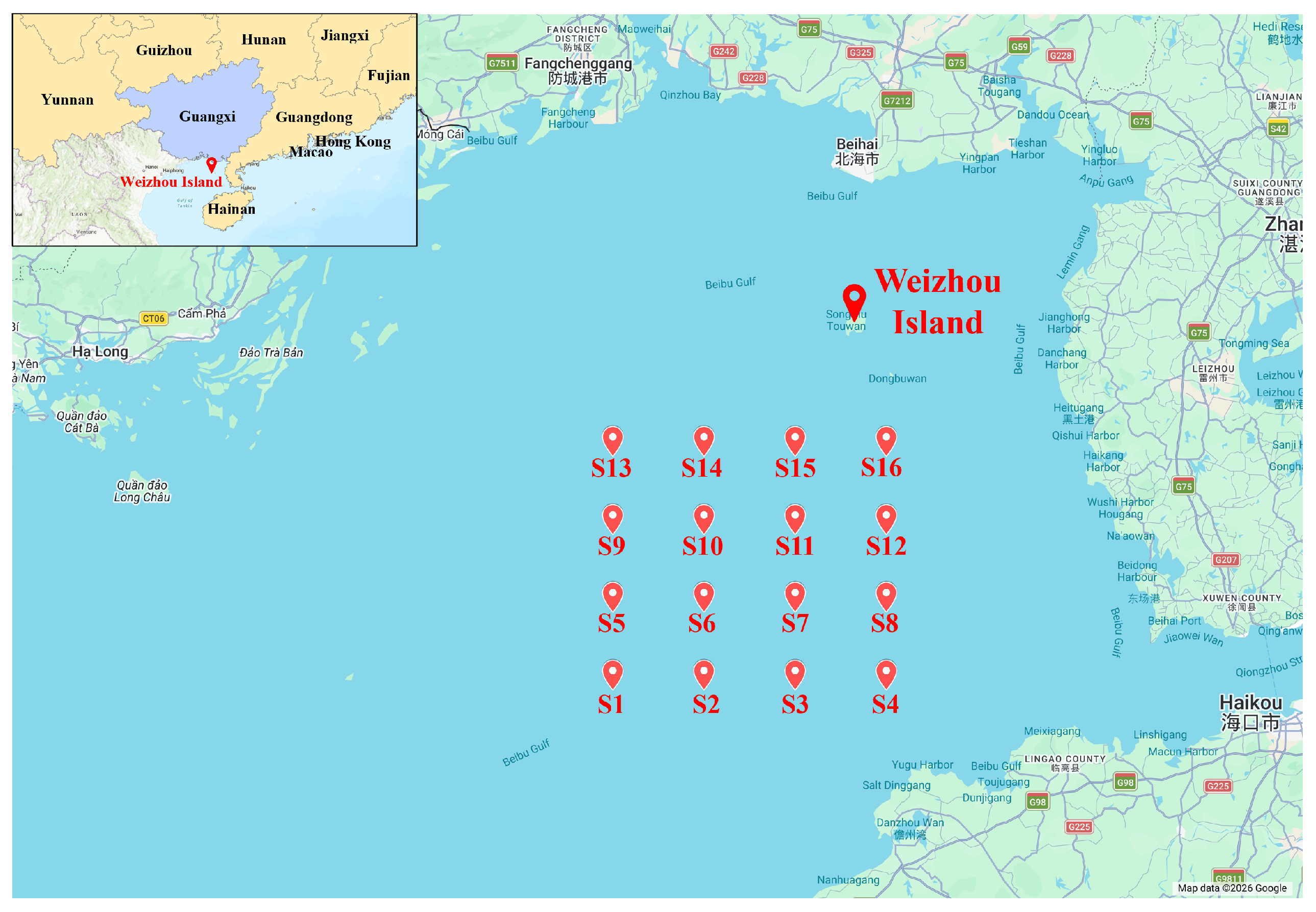
The study area is the Beibu Gulf, located in the northwestern part of the South China Sea. This region has strong potential for offshore renewable energy development. To support the analysis, we established a spatial grid consisting of 16 deep-sea locations.

These grid locations are labeled from S1 to S16 and are distributed along the offshore boundary facing the open sea. As shown in Figure 1, these locations were selected to represent typical offshore conditions and to capture the long-term variation of wind and solar resources in deep-water areas.

3.2. Raw Weather Data Acquisition and Processing

To construct the weather dataset, raw meteorological data were obtained from the NASA Prediction of Worldwide Energy Resources (POWER) database (https://power.larc.nasa.gov, accessed on 25 March 2026). This platform was selected due to its provision of reliable, satellite-derived hourly weather data with global coverage and long-term temporal consistency. In addition, it allows direct access to point-based time series in structured formats, making it particularly suitable for site-specific offshore resource assessment. The key variables, including 10 m wind speed, 10 m wind direction, solar irradiance, and 2 m air temperature, were collected for a 10-year period from 2016 to 2025.

A common issue in raw data extraction is that occasional satellite transmission errors lead to missing values, which are originally recorded as −999. In this marine dataset, such missing data are particularly challenging because they often span several consecutive days rather than appearing as isolated hourly gaps.

Applying standard mathematical methods, such as linear interpolation, to fill these multi-day gaps is physically inappropriate. For instance, interpolation over a two-day gap may produce non-zero solar irradiance during nighttime, thereby distorting the inherent diurnal cycle. To address this issue and preserve physically consistent weather patterns, a 24 h periodic substitution algorithm is proposed. For clarity and reproducibility, the detailed procedure of this method is presented in Algorithm 1.

Algorithm 1 Parameters and procedure of the 24 h periodic substitution algorithm

1: Input: Hourly time series $X\left(t\right)$ with missing values (NaN)   2: Output: Repaired time series $\tilde{X}\left(t\right)$   3: Step 1: Data preprocessing   4: Convert invalid values (e.g., $-999$) in $X\left(t\right)$ to NaN   5: Step 2: Missing data repair   6: for each time step t do   7:     if $X\left(t\right)\ne \mathrm{NaN}$ then   8:           $\tilde{X}\left(t\right)\leftarrow X\left(t\right)$   9:     else 10:           $k\leftarrow 1$ 11:           while true do 12:              if $X(t-24k)\ne \mathrm{NaN}$ then 13:                    $\tilde{X}\left(t\right)\leftarrow X(t-24k)$ 14:                    break 15:              else if $X(t+24k)\ne \mathrm{NaN}$ then 16:                    $\tilde{X}\left(t\right)\leftarrow X(t+24k)$ 17:                    break 18:              else 19:                    $k\leftarrow k+1$ 20:              end if 21:           end while 22:     end if 23: end for 24: Step 3: Output 25: return$\tilde{X}\left(t\right)$

During preprocessing, all −999 values are first converted into NaN (Not a Number). The algorithm then scans the complete 87,672 h time series. When a missing value is encountered, the algorithm first retrieves the corresponding value from 24 h earlier. If this value is also unavailable, it searches forward in 24 h increments until a valid observation is found.

To ensure the reliability of the dataset, a quantitative assessment of missing data was performed before imputation. Across the entire dataset (16 sites × 87,672 h), the total missing rates were extremely low, with 0.003% for wind speed (48 missing hours), 0.014% for solar irradiance (192 missing hours), and 0.027% for air temperature (384 missing hours). Missing values were uniformly distributed across all 16 sites. All missing values appeared in 24 h continuous blocks, with a maximum continuous gap of 24 h. Given this specific missing pattern, linear interpolation would fail to fill a complete 24 h gap, resulting in unusable data for that period. In contrast, the proposed 24 h periodic substitution method directly uses observations from the same hour of the previous day to fill the gap, effectively recovering complete diurnal cycles while maintaining physical consistency. Therefore, the 24 h periodic substitution method is the optimal choice for the missing data pattern of this dataset.

This cycle-based approach effectively reconstructs extended data gaps while preserving the inherent diurnal characteristics of meteorological variables, such as midday solar peaks and nighttime temperature declines. By applying this method to all 16 spatial grid points, the final Historical Weather Dataset is obtained.

3.3. Wind Power Physical Model

While the weather dataset provides the environmental conditions, calculating the electrical power output requires specific physical equations. For the wind power generation, the actual wind speed values from the Historical Weather Dataset serve as the primary input.

Because wind speed is measured at a reference height ($h_{ref}$) of 10 m, but the wind turbine hub is located at a much higher elevation (h), height correction is necessary. The standard power-law wind profile model is applied for this vertical adjustment [24]:

$$v\left(t\right)=v_{ref}\left(t\right){\left({\displaystyle \frac{h_{WT}}{h_{ref}}}\right)}^{\alpha }$$

(1)

where $v\left(t\right)$ represents the corrected wind speed reaching the hub height at time t, and $v_{ref}\left(t\right)$ is the original measured wind speed.

Next, the raw power output ($P_{WT}^{max}$) is calculated based on the technical limits of the representative commercial wind turbine. The power generation dynamically adjusts depending on three different operational wind speed zones (cut-in, rated, and cut-out) [25]:

$$P_{WT}^{max}\left(t\right)=\left\{\begin{array}{cc}0,\hfill & v\left(t\right)<v_{in}\mathrm{or}v\left(t\right)>v_{off}\hfill \\ {\displaystyle \frac{1}{2}}{C}_p{\eta }_{WT}{\rho }_{WT}\pi {\left({\displaystyle \frac{D}{2}}\right)}^{2}v{\left(t\right)}^3,\hfill & v_{in}\le v\left(t\right)<v_n\hfill \\ P_{WT}^{rated},\hfill & v_n\le v\left(t\right)\le v_{off}\hfill \end{array}\right.$$

(2)

Finally, to make the data directly comparable across different wind turbines, the raw output is divided by the rated wind capacity ($P_{WT}^{rated}$). This step produces the normalized wind power generation in per-unit (p.u.) values:

$$P\_WIND\left(t\right)={\displaystyle \frac{P_{WT}^{max}\left(t\right)}{P_{WT}^{rated}}}$$

(3)

Table 3. Parameters of the representative wind turbine model (based on a typical 8.5 MW low-wind-speed architecture e.g., MySE 8.5-230).

Parameter	Meaning	Value	Unit
$C_p$	Equivalent Power coefficient	$2.52 \times {10}^{-4}$	–
${\eta }_{WT}$	Electromechanical conversion efficiency	0.92	–
${\rho }_{WT}$	Air density	1.225	kg/m3
D	Rotor diameter	230	m
A	Swept area	$4.1548 \times {10}^4$	m2
$P_{WT}^{rated}$	Rated power	8.5	MW
$v_{in}$	Cut-in wind speed	3	m/s
$v_n$	Rated wind speed	11.3	m/s
$v_{off}$	Cut-out wind speed	25	m/s
$h_{WT}$	Hub height	155	m
$h_{ref}$	Reference measurement height	10	m
$\alpha$	Wind shear exponent	0.12 [24]	–

summarizes the specific parameters used for this representative wind turbine model.

3.4. PV Thermal-Thermodynamic Model

Just as the wind model translates weather variables into mechanical energy, the solar power generation is calculated using solar irradiance (G), air temperature ($T_a$), and environmental wind speed ($v_{ref}$) extracted directly from the Historical Weather Dataset.

A critical environmental factor in marine settings is that offshore solar arrays are typically installed very close to the sea surface. Consequently, the local cooling wind speed $v_{PV}\left(t\right)$ at the PV panel height ($h_{PV}$) differs from the wind speed reaching the towering turbine hub. To accurately address this, the power-law correction must first be applied to determine the exact wind speed hitting the solar panels:

$$v_{PV}\left(t\right)=v_{ref}\left(t\right){\left({\displaystyle \frac{h_{PV}}{h_{ref}}}\right)}^{\alpha }$$

(4)

Using this corrected wind speed, the actual physical temperature of the solar PV cells ($T_c$) is determined. This specific thermodynamic model evaluates both the heating load from direct sunlight and the essential convection cooling effect from the crosswinds ($v_{PV}$) flowing across the panel surfaces [26]:

$$T_c\left(t\right)=T_a\left(t\right)+{\displaystyle \frac{G\left(t\right)}{800}}(NOCT-20){\displaystyle \frac{9.5}{5.7+3.8v_{PV}\left(t\right)}}$$

(5)

Once the cell temperature is established, the raw solar power output ($P_{PV}^{max}$) is computed. A key feature of this equation is its ability to precisely measure the power generation losses that naturally occur when panels overheat under intense irradiation [27]:

$$P_{PV}^{max}\left(t\right)=P_{PV}^{rated}{\displaystyle \frac{G\left(t\right)}{G_{STC}}}\left[1+\gamma \left(T_c\left(t\right)-T_{STC}\right)\right]$$

(6)

Finally, to align with the normalized format introduced in Section 2, the raw physical output is divided by the rated solar capacity ($P_{PV}^{rated}$). This final conversion produces the normalized solar power yield on a per-unit (p.u.) basis:

$$P\_PV\left(t\right)={\displaystyle \frac{P_{PV}^{max}\left(t\right)}{P_{PV}^{rated}}}$$

(7)

Table 4. Parameters of the representative solar PV model.

Parameter	Meaning	Value	Unit
$P_{PV}^{rated}$	Rated capacity of PV array	4.5	MW
$G_{STC}$	Solar irradiance at standard test conditions	1000 [27]	W/m2
$T_{STC}$	Cell temperature at standard test conditions	25 [27]	°C
$\gamma$	Power temperature coefficient	−0.0038 [28]	1/°C
$NOCT$	Nominal operating cell temperature	49 [29]	°C
$h_{ref}$	Reference measurement height	10	m
$h_{PV}$	Specific installation height of PV arrays	2	m

details all the required parameters for the representative commercial solar PV arrays.

By applying these sequential physical models for all hours across the decade, the complete Normalized Power Yield Dataset is constructed.

3.5. Assumptions, Limitations, and Sensitivity Analysis of the Representative Models

The representative wind turbine (based on an 8.5 MW low-wind-speed model, e.g., MySE 8.5-230) and PV model (based on standard crystalline silicon panels) rely on several key assumptions. For wind power, the power curve follows a simple three-zone (cut-in, rated, cut-out) formulation without considering yaw misalignment, wake effects, or blade wear; air density is fixed at 1.225 kg/m³; and the wind shear exponent $\alpha$ is taken as 0.12, representing neutral conditions over open water. For PV power, the NOCT-based cooling coefficient comes from on-land installations and may not fully apply to floating offshore systems; the temperature coefficient $\gamma$ is assumed constant; and soiling, spectral mismatch, and long-term degradation are not considered.

These assumptions mean the models are not universally applicable. Geographically, the models are calibrated for the Beibu Gulf’s subtropical marine climate; applying them to other regions (e.g., tropical cyclone areas or high-latitude waters) may cause bias. Technologically, the turbine (8.5 MW, 230 m rotor) and PV panel (crystalline silicon) represent mainstream equipment in China as of 2022; for very different designs (e.g., 15 MW+ turbines or thin-film PV), users should replace the core power curves or temperature-loss equations while keeping the weather data unchanged. Temporally, the 10-year period (2016–2025) captures year-to-year variations but does not cover long-term climate trends beyond this window.

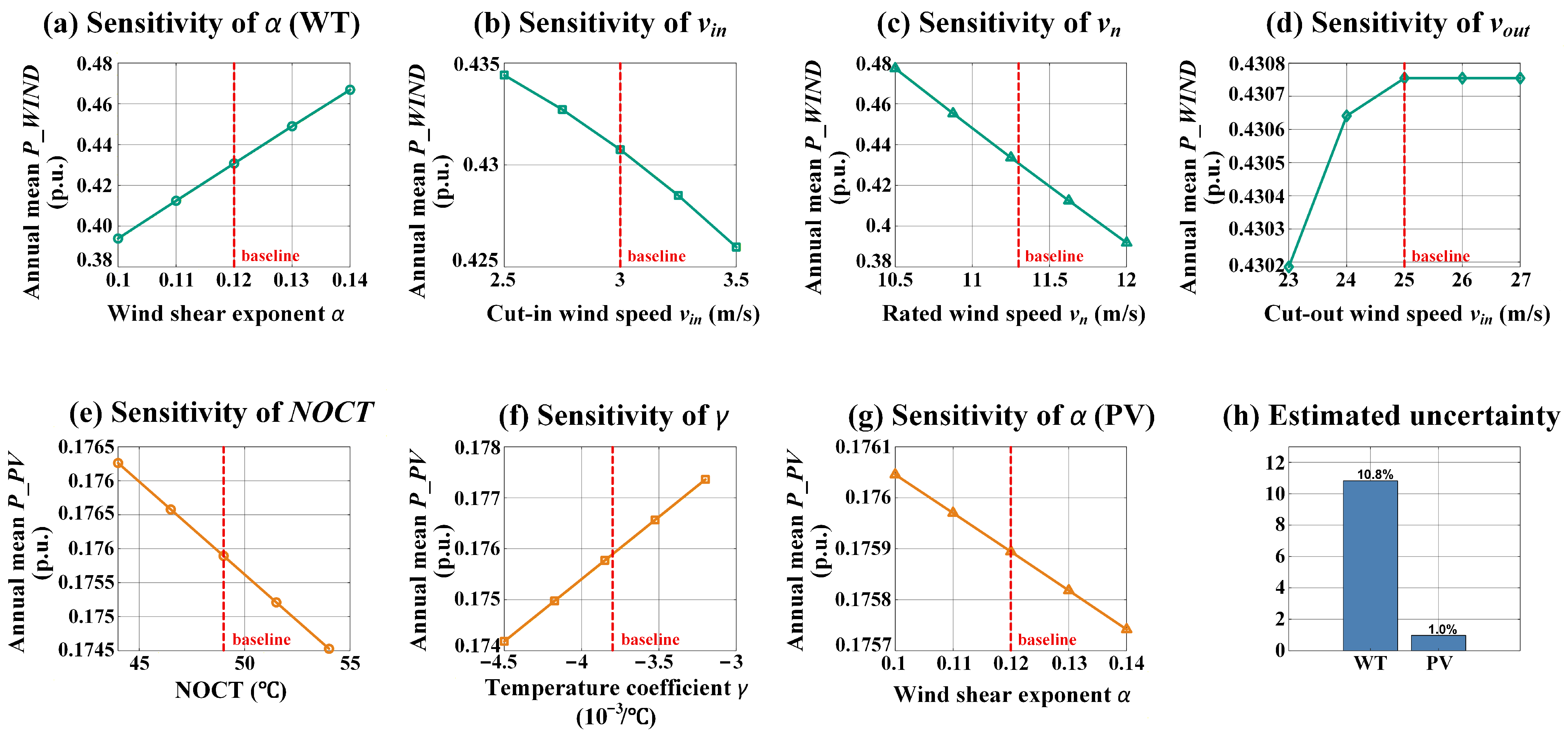
To measure the impact of uncertain parameters, a one-at-a-time sensitivity analysis was performed using hourly data from a representative site (S1) over one full year (2020). As shown in Figure 2, varying the wind shear exponent $\alpha$ from 0.10 to 0.14 changes $P_{\mathrm{WIND}}$ by approximately $\pm 0.036$ p.u.; varying the rated wind speed $v_n$ from 10.5 to 12.0 m/s changes $P_{\mathrm{WIND}}$ by −0.039 to +0.047 p.u.; while the cut-in and cut-out wind speeds have much smaller effects (<±0.005 p.u.). For the PV model, varying NOCT from 44 °C to 54 °C or varying the temperature coefficient $\gamma$ from −0.0045 to −0.0032 °C⁻¹ changes $P_{\mathrm{PV}}$ by less than $\pm 0.002$ p.u., and the wind shear exponent for PV panels (${\alpha }_{\mathrm{pv}}$) has a negligible effect ($\pm 0.0002$ p.u.).

Based on these results, the estimated relative uncertainty of the annual average normalized output is approximately $\pm 10.8\%$ for wind power, mainly driven by the rated wind speed $v_n$ and the wind shear exponent $\alpha$. In contrast, the PV output uncertainty is only about $\pm 1.0\%$, indicating that the PV model is highly robust to parameter variations within the tested ranges. For comparative studies such as site ranking or wind–solar ratio optimization, the ranking uncertainty is expected to be much lower than these absolute uncertainty estimates, because parameter variations affect all sites in similar ways. Therefore, the dataset remains well suited for relative comparisons and hybrid system design, while users seeking high absolute accuracy in wind power estimates should calibrate $\alpha$ and $v_n$ using local measurements. The detailed sensitivity analysis results are summarized in

Table 5. Sensitivity analysis of key model parameters.

Parameter	Symbol	Baseline	Range	$\mathbf{\Delta }$ Annual Mean (p.u.)
Wind power model
Wind shear exponent	$\alpha$	0.120	0.10–0.14	−0.0368 to +0.0362
Cut-in wind speed	$v_{\mathrm{in}}$	3.0 m/s	2.5–3.5 m/s	−0.0048 to +0.0037
Rated wind speed	$v_{\mathrm{n}}$	11.3 m/s	10.5–12.0 m/s	−0.0389 to +0.0466
Cut-out wind speed	$v_{\mathrm{out}}$	25.0 m/s	23.0–27.0 m/s	−0.0006 to +0.0000
PV power model
Nominal operating cell temperature	NOCT	49.0 °C	44–54 °C	−0.0014 to +0.0014
Temperature coefficient	$\gamma$	−0.0038 °C−1	−0.0045 to −0.0032 °C−1	−0.0017 to +0.0015
Wind shear exponent (PV)	$\alpha$	0.120	0.10–0.14	−0.0002 to +0.0002

.

4. Data Exploration and Evaluation

This dataset provides a foundation for analyzing offshore marine environments and renewable power generation. To better understand the data and confirm its quality, a technical evaluation was performed across the 16 deep-sea grids.

The evaluation process is organized into three main areas. First, Section 4.1 analyzes the overall distribution of the basic weather resources, such as wind speed and solar irradiance. Second, Section 4.2 explores extreme weather conditions, highlighting the actual equipment limits and the forced shutdown hours. Finally, Section 4.3 examines the calculated power yield, focusing on the expected energy generation and the daily fluctuation curves. The details of these three evaluation steps are presented below.

4.1. Overall Evaluation of Marine Renewable Resources

This section involves gaining an understanding of the environmental baseline by evaluating the statistical and temporal distributions of the weather variables. To ensure operational accuracy, all wind speed records in this section are adjusted to the 155-m turbine hub height using the standard power-law equation.

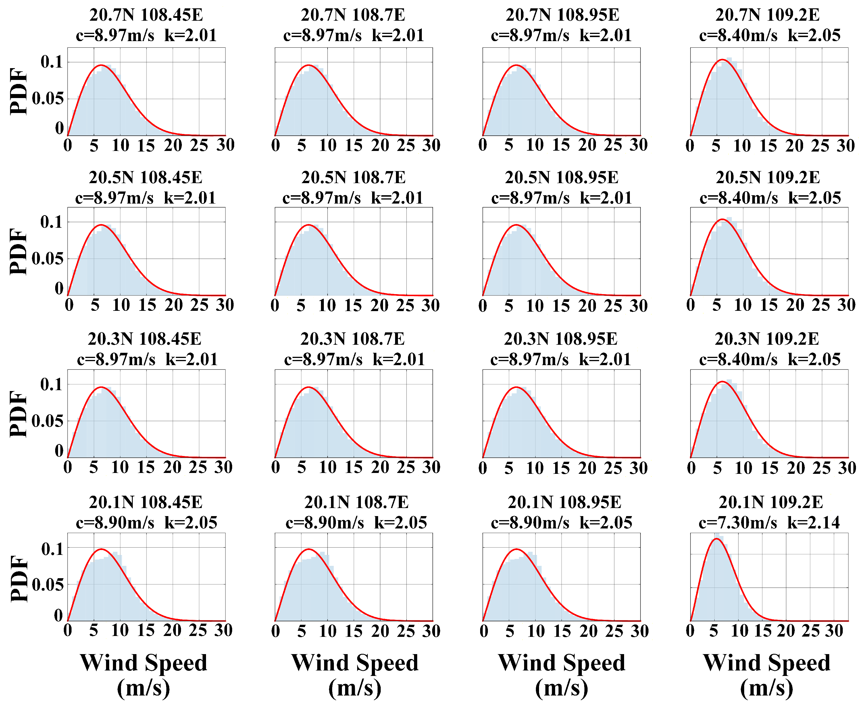
Initially, probability models were used to identify the basic wind characteristics across the 16 deep-sea grids. As presented in Figure 3, the Weibull distribution was applied to the hourly wind speed data for each site. The analysis reveals that wind speeds consistently follow common right-skewed distribution curves. This confirms the spatial reliability of the wind data across the entire Beibu Gulf array.

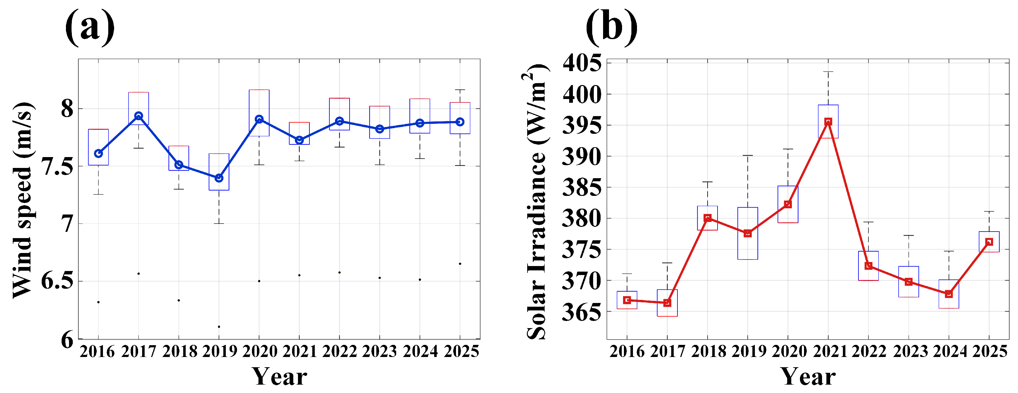
Furthermore, the 10-year continuous records allow for temporal evaluations across three specific scales: inter-annual, seasonal, and daily. To verify long-term data continuity, the inter-annual variation over the 10-year span (2016–2025) is evaluated in Figure 4. The results indicate that both wind speed and solar irradiance exhibit overall year-to-year stability, while showing moderate inter-annual fluctuations, such as higher wind speeds in 2017 and lower in 2019, and a peak in solar irradiance in 2021. These observations indicate that the annual mean values in the dataset are generally consistent, without any unusually large deviations over the 10-year period.

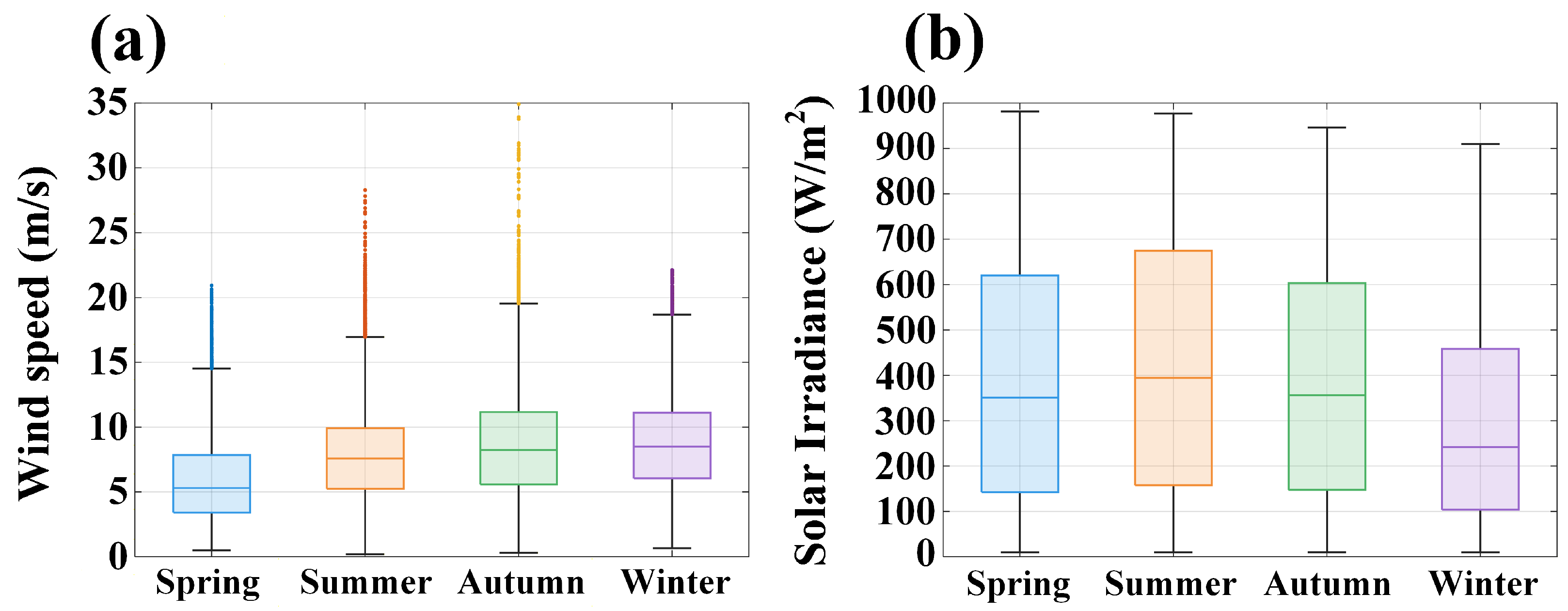
In addition to annual stability, distinct seasonal patterns are observed. Figure 5 highlights the contrast between the strong marine winds in winter and the intense solar irradiance in summer (evaluated exclusively during daylight hours, $G > 10$ W/m²).

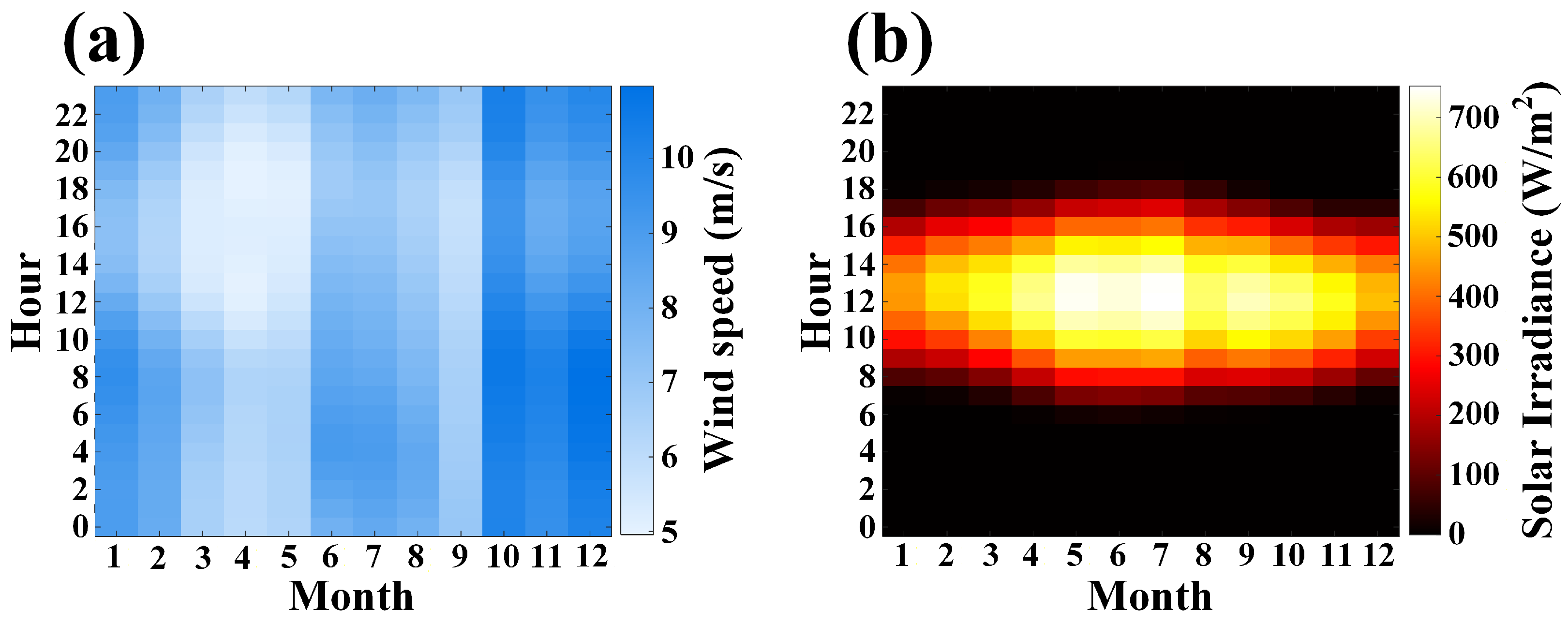
Finally, to analyze the monthly and daily patterns of the deep-sea resources in more detail, a month-hour heatmap is presented in Figure 6. To show the overall regional condition, this chart uses the average data of all 16 sites. It tracks the 24 h resource changes across different months, clearly showing the specific times when wind speeds peak and when solar energy is available. Together, these basic evaluations confirm that the dataset correctly records the complex weather patterns of the marine environment, making it a reliable base for future power modeling.

The observed spatial patterns can be explained by the geographical characteristics of the Beibu Gulf. Sites S1–S3, located further offshore, experience less land surface friction and more stable marine boundary layers, resulting in higher and more consistent wind speeds compared to nearshore sites such as S4 and S12. For solar irradiance, the high spatial uniformity across all 16 sites reflects the relatively small geographical span of the study area (0.75° in longitude and 0.6° in latitude), over which cloud cover and atmospheric attenuation exhibit minimal variation. The seasonal patterns shown in Figure 5 are primarily driven by the East Asian monsoon system: strong northeasterly winds prevail in winter, while summer brings weaker winds but higher solar altitude angles and longer daylight hours, creating a natural seasonal complementarity between wind and solar resources.

4.2. Extreme Weather Analysis Across Spatial Grids

This section evaluates the continuous 10-year dataset to quantify the extreme weather conditions across the 16 marine grids. The definitions for extreme high and low wind events are based directly on the operational limits of the representative wind turbine model. Specifically, a low-wind shutdown (calm period) is defined as any hour when the wind speed drops below the 3 m/s cut-in threshold. An extreme high-wind shutdown (typhoon lockdown) is recorded when the wind speed exceeds the 25 m/s cut-out limit, forcing the turbine’s safety protection system to stop power generation. For the solar arrays, extreme thermal conditions are tracked using the PV thermodynamic model to identify periods when the cell temperature ($T_c$) climbs above the 50 °C danger limit.

Table 6. The 10-Year extreme weather and equipment operational boundary summary for the 16 deep-sea grids.

Site	Max Wind	Typhoon	Max Cont.	Calm	Max Cont.	Max Cell	Hours	Max Eff.
	Speed (m/s)	Shutdown (h)	Typhoon (h)	Shutdown (h)	Calm (h)	Temp (°C)	${\mathit{T}}_{\mathit{c}} > \mathbf{50°}$C (h)	Loss (%)
S1	34.14	53	12	9937	53	78.7	1733	20.39
S2	34.14	53	12	9937	53	78.7	1733	20.39
S3	34.14	53	12	9937	53	78.7	1733	20.39
S4	34.36	36	11	11,094	48	89.2	3139	24.39
S5	36.46	61	13	9548	52	78.4	1497	20.29
S6	36.46	61	13	9548	52	78.4	1497	20.29
S7	36.46	61	13	9548	52	78.4	1497	20.29
S8	39.02	69	16	10,278	43	82.9	2249	22.00
S9	36.46	61	13	9548	52	78.4	1497	20.29
S10	36.46	61	13	9548	52	78.4	1497	20.29
S11	36.46	61	13	9548	52	78.4	1497	20.29
S12	39.02	69	16	10,278	43	82.9	2249	22.00
S13	36.46	61	13	9548	52	78.4	1497	20.29
S14	36.46	61	13	9548	52	78.4	1497	20.29
S15	36.46	61	13	9548	52	78.4	1497	20.29
S16	39.02	69	16	10,278	43	82.9	2249	22.00

summarizes these worst-case weather scenarios for each individual site. The table extracts the absolute maximum wind speeds and the longest continuous shutdown periods caused by both typhoons and dead winds. It also reports the maximum peak temperatures that the solar cells endured, along with the highest instantaneous efficiency loss recorded during the 10-year span.

4.3. Model-Based Power Yield and Output Fluctuation

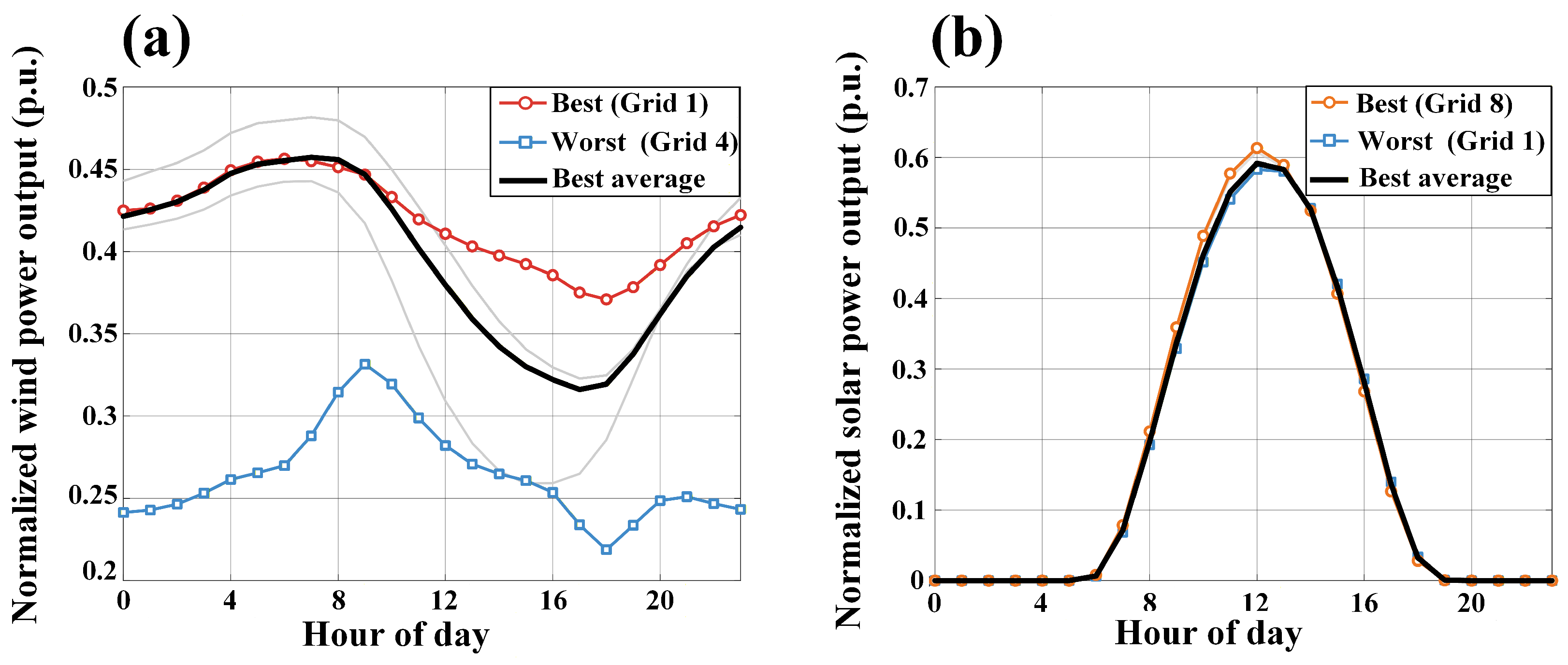
This section applies the wind and solar physical models from Section 3 to calculate the normalized power output for all 16 sites. All results are expressed on a 1.0 per-unit (p.u.) base relative to the rated capacity of each equipment type. To illustrate the typical daily generation behavior, the hourly normalized outputs are averaged across the full 10-year period. Figure 7 presents the resulting diurnal curves for all 16 sites.

For wind power, a clear daily pattern is observed: output rises to a morning peak near 08:00, then falls to a lower afternoon trough around 16:00–18:00 before partially recovering at night. A considerable spread exists between the best-performing site (Grid 1, ≈0.45 p.u.) and the worst (Grid 4, ≈0.25 p.u.), indicating notable spatial variability in wind resources across the region. This spatial variability is primarily attributed to differences in offshore distance. Grid 1, located further offshore with a longer fetch, experiences higher wind speeds than Grid 4, which is closer to the Leizhou Peninsula, where land friction reduces winds. The diurnal wind pattern (morning peak, afternoon trough) reflects typical land-sea thermal circulation. Daytime heating of the land creates onshore winds that are partially blocked by coastal terrain, while nighttime cooling allows more stable offshore flow.

For solar PV, the output is zero during nighttime, rises steadily from sunrise, reaches a single peak near solar noon, and returns to zero after sunset. In contrast to wind, the solar profiles of all 16 sites are nearly identical, which occurs because the study area’s small spatial span (approximately 0.75° in longitude and 0.6° in latitude) leads to minimal variations in cloud cover and atmospheric attenuation.

Overall, the wind and solar generation profiles exhibit a natural time-complementary relationship, where wind contributes during the night and early morning while solar dominates the midday period. This inverse diurnal pattern, combined with the seasonal complementarity shown in Figure 5 (strong winter winds vs. abundant summer solar), suggests strong potential for hybrid wind–solar development in this region, as the two resources naturally balance each other across both daily and seasonal cycles.

5. User Notes and Advanced Applications

All data files from both sub-datasets are stored in CSV format with UTF-8 encoding and are suitable for importing to virtually any data processing software. The Historical Weather Dataset consists of 16 individual CSV files, and the Normalized Power Yield Dataset consists of a further 16 CSV files, with each file corresponding to one specific deep-sea grid site. The complete dataset can be freely accessed without logging in at https://github.com/Lee-ziniu/10-Year-Hourly-Offshore-Weather-and-Wind-Solar-Power-Dataset-for-the-Beibu-Gulf.git (accessed on 1 April 2026). A wide range of analytical models and engineering frameworks can be implemented using this dataset. To demonstrate its practical value, two representative application cases are presented below, covering offshore array siting and capacity design, and physics-informed deep learning forecasting.

5.1. Array Siting and Capacity Design Examples

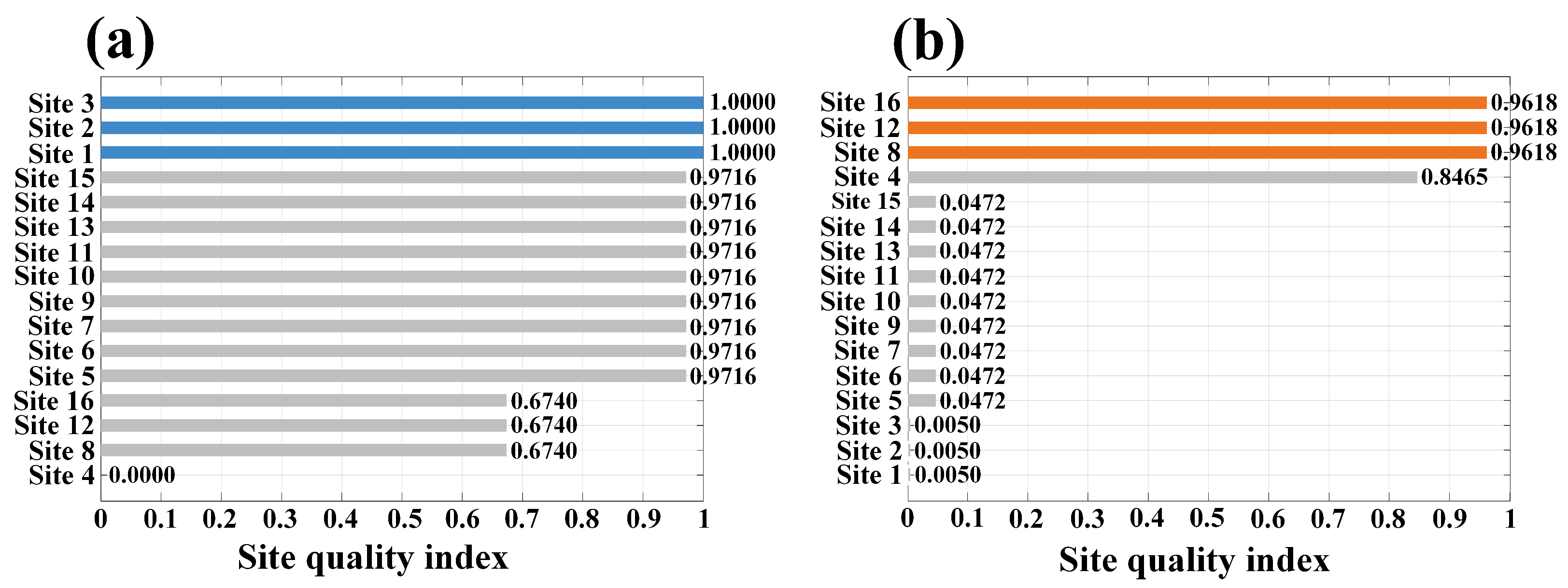
This case demonstrates how the Normalized Power Yield Dataset can be used to guide the spatial siting and capacity configuration of an offshore hybrid wind–solar power plant. For site selection, a composite Site Quality Index (SQI) is constructed for each of the 16 marine grids. The index assigns a 70% weight to the normalized annual Equivalent Full Load Hours (EFLH) and a 30% weight to the normalized generation stability, measured by the inverse of the coefficient of variation (CV). As shown in Figure 8, by ranking all sites using this index, sites S1, S2, and S3 receive the highest wind SQI scores (1.0) and are therefore selected for wind farm deployment. For solar PV, sites S8, S12, and S16 achieve the highest solar SQI scores (0.9618) and are selected for solar array deployment.

The selection of S1–S3 for wind deployment is explained by their offshore locations with longer fetches and minimal land interference, as discussed in Section 4.3. For solar deployment, S8, S12, and S16 achieve the highest scores not because of higher irradiance, which is nearly uniform across all sites, but because of slightly better cooling conditions including lower ambient temperatures and higher 2-m wind speeds that improve conversion efficiency. This demonstrates that even small spatial variations in wind speed can influence PV performance through the cooling effect, an insight that would be missed if only irradiance were considered.

For capacity sizing, the average normalized outputs of the three selected wind sites and the three selected solar sites are taken as the representative generation profiles. A systematic scan is then performed over the full wind-to-solar installed capacity ratio range (0–100%) in 1% increments. At each ratio, the CV of the combined hybrid output is calculated. The ratio that produces the lowest CV, corresponding to the smoothest overall power output, is identified as the optimal configuration. This search yields an optimal wind-to-solar ratio of approximately 49%:51%.

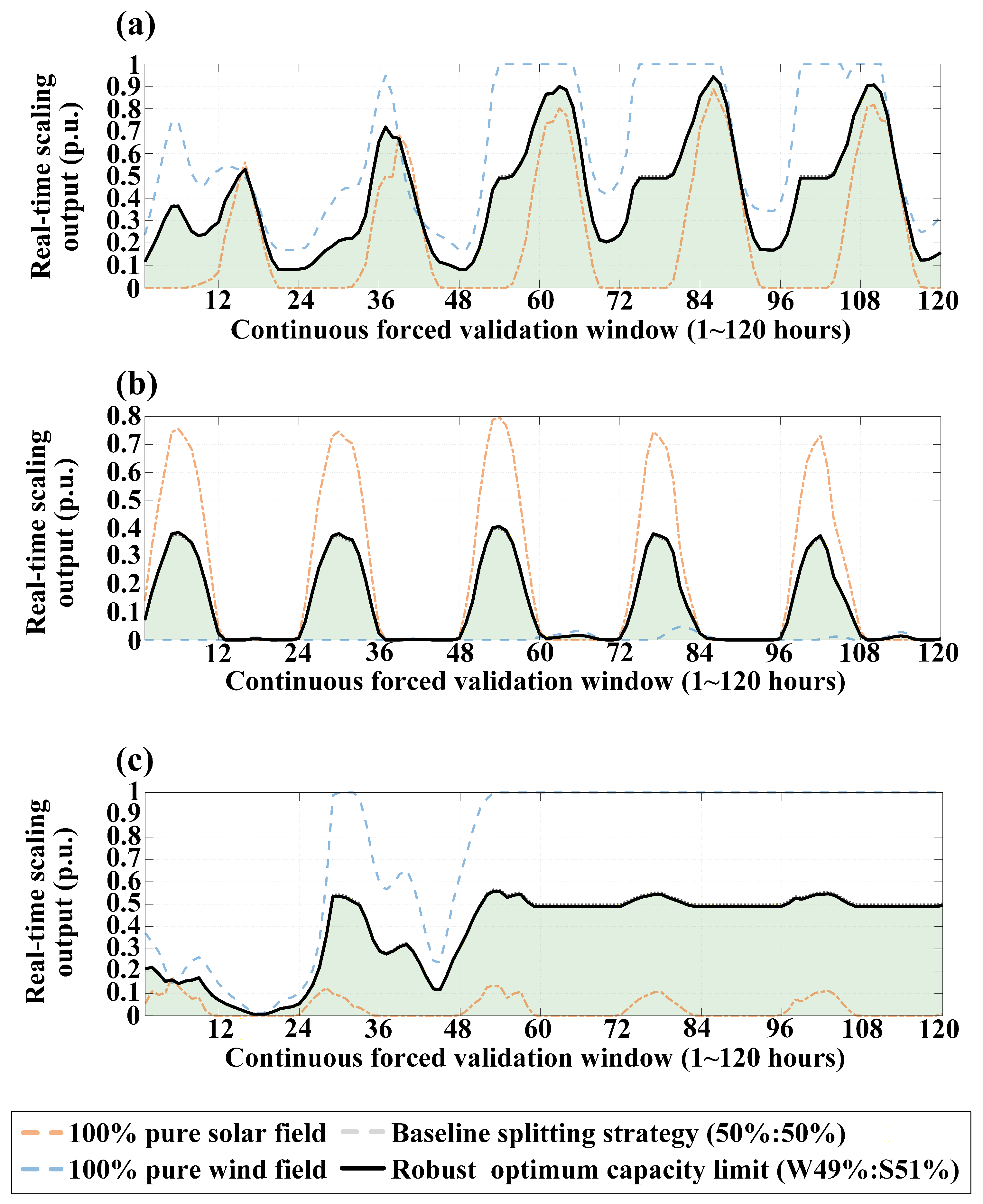
To validate this configuration under extreme real-world conditions, three independent 120-h (5-day) stress tests are conducted using historical data windows automatically extracted from the dataset. As shown in Figure 9, the three scenarios cover normal weather alternation, extreme wind drought combined with intense heat, and a dark overcast period with turbulent storms. Across all three scenarios, the optimized 49:51 configuration consistently achieves a lower output fluctuation (CV) compared to a pure wind array, a pure solar array, or a naive 50:50 split. In particular, under the extreme wind drought scenario (Scenario B), the pure wind array collapses to a near-zero mean output of 0.0051 p.u., while the optimized hybrid configuration maintains a mean output of 0.1163 p.u. with a significantly reduced peak-to-valley range.

5.2. Deep Learning and Physics-Driven Forecasting

This case demonstrates the compatibility of the dataset with physics-informed deep learning models for both long-term trend projection and short-term operational forecasting.

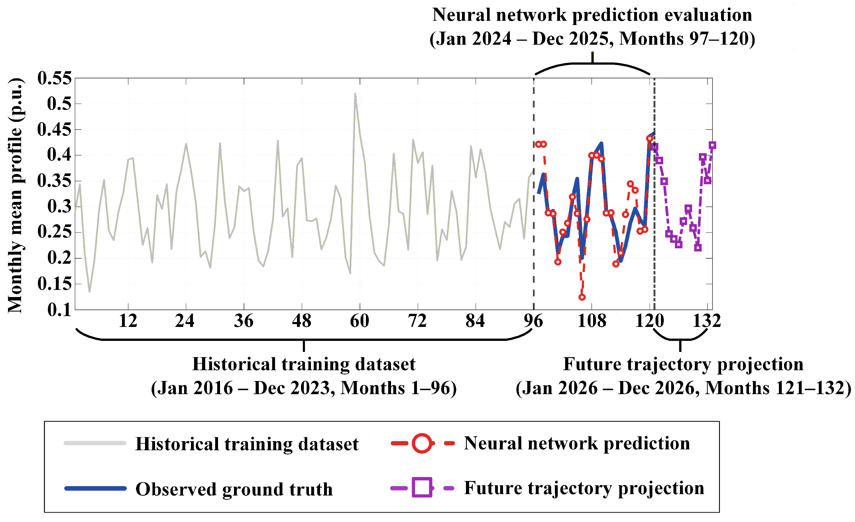
For macro-scale analysis, a Long Short-Term Memory (LSTM) network is trained to predict the monthly mean normalized hybrid power output (p.u.) of the optimized 49:51 configuration. LSTM is a type of recurrent neural network designed to capture long-range dependencies in sequential data. The input at each monthly step consists of three features: the previous month’s power output and a pair of sine–cosine encodings representing the calendar month, which allow the model to recognize seasonal cycles directly. The dataset is split into an 8-year training period (January 2016–November 2023) and a 2-year independent test period (November 2023–December 2025), followed by a 12-month forward projection for 2026. To prevent the model from losing its seasonal memory at the train-test boundary, a State Priming mechanism is applied, where the hidden state accumulated during the full training pass is carried over directly into the test phase rather than being reset. As shown in Figure 10, this allows the model to track the seasonal generation cycle continuously across the boundary without any visible discontinuity, accurately reproducing the peaks and troughs of the 2-year blind test period. Quantitatively, the reconstructed hybrid power output achieves an RMSE of 0.018 p.u. and an R² of 0.94 over the 72 h test period, confirming the forecasting capability supported by the dataset.

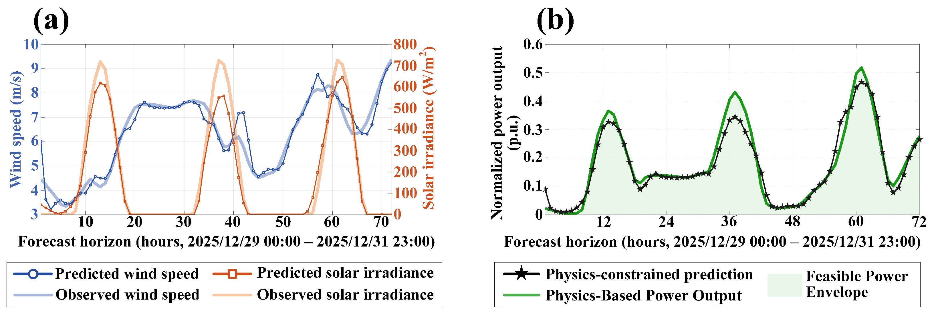
For micro-scale analysis, a second LSTM network is trained to simultaneously predict three hourly meteorological variables (wind speed, solar irradiance, and air temperature) using the last 1440 h (approximately 60 days) of the dataset. Rather than predicting power output directly, the model takes an 8-dimensional input at each time step: the previous hour’s meteorological values, the corresponding 24 h-lagged values capturing the diurnal periodicity, and a sine–cosine pair encoding the current hour of the day. This diurnal phase encoding gives the network explicit awareness of daylight hours, which forces the predicted solar irradiance to return correctly to zero at night. The final 72 h (29–31 December 2025) are held out as the test set. After prediction, the three forecast meteorological variables are passed through the complete physical model chain from Section 3, including height correction, PV cell temperature calculation, wind turbine power curve, and the optimized 49:51 capacity ratio, to reconstruct the final hybrid power output. As shown in Figure 11, the predicted meteorological profiles closely follow the measured values, and the physics-constrained power output remains within the correct operational boundaries throughout the 72 h test window.

Together, these two cases confirm that the 10-year continuous hourly records in this dataset provide sufficient temporal depth for sequential deep learning models, while the normalized physical outputs ensure that all reconstructed power predictions remain bounded within realistic engineering constraints.

6. Conclusions

The value of this dataset extends beyond its immediate engineering applications. It fills a clear gap in the current literature by providing a rare combination of long-term, high-resolution, and spatially distributed offshore weather and power generation records for a region that has rarely been covered by existing open-access databases. The 10-year continuous hourly records across 16 deep-sea sites in the Beibu Gulf offer a level of detail and temporal depth that is difficult to find in similar public datasets for the South China Sea region.

This wealth of structured data opens up a range of research opportunities. It enables researchers to study offshore climate variations, evaluate physical power generation models, and develop data-driven forecasting methods. The two application cases presented in this paper illustrate that the dataset can be effectively used with both engineering optimization workflows and modern deep learning models, suggesting that the data is well structured and suitable for model training and testing tasks.

The normalization of all power outputs to a 1.0 p.u. basis, combined with the open CSV format and UTF-8 encoding, ensures that the dataset is accessible to a broad range of users, from energy planners and power system engineers to machine learning researchers. By making this dataset freely available, this work aims to provide a reliable and practical foundation for advancing offshore renewable energy research, supporting studies across different marine environments, and facilitating progress in hybrid wind–solar system planning and intelligent energy forecasting.

Beyond the dataset description, several analytical insights emerge from our evaluation. The spatial variability of wind resources (CV ≈ 15%) is considerably higher than that of solar resources (CV < 2%), indicating that site selection is more critical for wind farms than for PV arrays. The observed seasonal complementarity between winter wind and summer solar suggests that hybrid systems may reduce storage requirements compared to single-source systems, though the exact reduction depends on specific system configurations and operational strategies. The sensitivity analysis shows that wind power estimates have an uncertainty of approximately ±10.8% (mainly from $v_n$ and $\alpha$), while PV estimates are more robust with an uncertainty of only ±1.0%. Therefore, users applying this dataset to other regions are encouraged to calibrate $\alpha$ and $v_n$ using local measurements, whereas the PV model can be used with higher confidence without site-specific calibration.

References

- Du, W.; Cai, G.; Zhang, J.; Li, Y.; Zhou, Z.; Chen, X.; Nie, S. An integrated spatiotemporal techno-economic assessment of offshore renewable energy complementarity: A case study in China’s maritime zones. Appl. Energy 2026, 410, 127513. [Google Scholar] [CrossRef] [Scilit]
- Kumar, S.; Panagant, N.; Arzaghi, E.; Baalisampang, T.; Garaniya, V.; Abbassi, R. A multi-objective optimisation framework for a standalone hybrid offshore renewable energy system with electrical and hydrogen loads. Energy 2025, 330, 136826. [Google Scholar] [CrossRef] [Scilit]
- Ma, Y.; Cui, L.; Zhou, H.; Bhattacharya, S. Hybrid offshore renewable energy harvest system: A review. Energy Convers. Manag. 2026, 348, 120654. [Google Scholar] [CrossRef] [Scilit]
- Liu, Y.; Liu, W.; Liu, J.; Zhang, H.; Li, Z.; Ban, M. Optimal operation strategy for multi-energy systems considering renewable energy fluctuation and carbon emission. Int. J. Electr. Power Energy Syst. 2025, 169, 110794. [Google Scholar] [CrossRef] [Scilit]
- Zhou, J.; Zhang, Z.; Zhang, R.; Zhang, W.; Xu, G.; Wang, H. Optimal capacity and multi-stable flexible operation strategy of green ammonia systems: Adapting to fluctuations in renewable energy. Energy Convers. Manag. 2024, 314, 118720. [Google Scholar] [CrossRef] [Scilit]
- Li, S.; Zhu, J.; Dong, H.; Zhu, H.; Fan, J. A novel rolling optimization strategy considering grid-connected power fluctuations smoothing for renewable energy microgrids. Appl. Energy 2021, 309, 118441. [Google Scholar] [CrossRef] [Scilit]
- Zhao, W.; Wang, J.; Huang, W.; Zhou, M.; Cao, J.; Li, Y. Revealing deep-far offshore wind potential through an integrated resource assessment and priority zoning framework: A case from China’s adjacent seas. Appl. Energy 2026, 413, 127790. [Google Scholar] [CrossRef] [Scilit]
- Gkeka-Serpetsidaki, P.; Dimitriou, I.C.; Poursanidis, D.; Xirouchakis, S.; Skiniti, G.; Tournaki, S.; Tsoutsos, T. Development of offshore wind farms from an environmental perspective. Renew. Energy 2026, 266, 125649. [Google Scholar] [CrossRef] [Scilit]
- Djalab, A.; Djalab, Z.; El Hammoumi, A.; Marco Tina, G.; Motahhir, S.; Laouid, A.A. A comprehensive review of floating photovoltaic systems: Tech advances, marine environmental influences on offshore PV systems, and economic feasibility analysis. Sol. Energy 2024, 277, 112711. [Google Scholar] [CrossRef] [Scilit]
- Vasuki, S.S.; Levell, J.; Simanjuntak, T.; Santbergen, R.; Isabella, O. Wave-induced losses in offshore floating PV: Physics-based modelling, sensitivity-driven quantification, surrogate-model prediction, and design-guided mitigation strategies. Energy Convers. Manag. X 2026, 30, 101723. [Google Scholar] [CrossRef] [Scilit]
- Ghosh, A. A comprehensive review of water based PV: Flotavoltaics, under water, offshore & canal top. Ocean Eng. 2023, 281, 115044. [Google Scholar] [CrossRef] [Scilit]
- Huang, J.; Iglesias, G. Hybrid offshore wind–solar energy farms: A novel approach through retrofitting. Energy Convers. Manag. 2024, 319, 118903. [Google Scholar] [CrossRef] [Scilit]
- Ali, F.; Stewart, R.A.; Sanjari, M.J.; Hayward, J.A.; Nicholson, R.C.; Etemad-Shahidi, A. A GIS-based framework for hybrid offshore wind and floating solar power plants in Australia. Ocean Coast. Manag. 2026, 277, 108199. [Google Scholar] [CrossRef] [Scilit]
- Frías-Paredes, L.; Gastón-Romeo, M. A new methodology to easy integrate complementarity criteria in the resource assessment process for hybrid power plants: Offshore wind and floating PV. Energy Convers. Manag. X 2025, 26, 100938. [Google Scholar] [CrossRef] [Scilit]
- Wang, J.; Zhang, Z.; Xu, W.; Li, Y.; Niu, G. Short-Term Photovoltaic Power Forecasting Using a Bi-LSTM Neural Network Optimized by Hybrid Algorithms. Sustainability 2025, 17, 5277. [Google Scholar] [CrossRef] [Scilit]
- Li, X.; Zhang, Y.; Wang, Z.; Song, Z. Short-Term Wind Power Prediction Based on Optimized VMD and LSTM. Energy Eng. 2025, 122, 4603–4619. [Google Scholar] [CrossRef] [Scilit]
- Solbrekke, I.M.; Sorteberg, A. NORA3-WP: A high-resolution offshore wind power dataset for the Baltic, North, Norwegian, and Barents Seas. Sci. Data 2022, 9, 362. [Google Scholar] [CrossRef] [Scilit]
- An, K.; Cai, W.; Lu, X.; Wang, C. High-resolution gridded dataset of China’s offshore wind potential and costs under technical change. Sci. Data 2025, 12, 69. [Google Scholar] [CrossRef] [Scilit] [PubMed]
- Xu, Y.; Lin, Y.; Li, S.; Gao, X. Prediction Model of Offshore Wind Power Based on Multi-Level Attention Mechanism and Multi-Source Data Fusion. Electronics 2025, 14, 3183. [Google Scholar] [CrossRef] [Scilit]
- Verdone, A.; Panella, M.; De Santis, E.; Rizzi, A. A review of solar and wind energy forecasting: From single-site to multi-site paradigm. Appl. Energy 2025, 392, 126016. [Google Scholar] [CrossRef] [Scilit]
- Parsa, S.M. Physics-informed machine learning meets renewable energy systems: A review of advances, challenges, guidelines, and future outlooks. Appl. Energy 2025, 402, 126925. [Google Scholar] [CrossRef] [Scilit]
- Gijón, A.; Eiraudo, S.; Manjavacas, A.; Schiera, D.S.; Molina-Solana, M.; Gómez-Romero, J. Integrating physics and data-driven approaches: An explainable and uncertainty-aware hybrid model for wind turbine power prediction. Comput. Phys. Commun. 2025, 316, 109761. [Google Scholar] [CrossRef] [Scilit]
- Meng, C.; Griesemer, S.; Cao, D.; Seo, S.; Liu, Y. When physics meets machine learning: A survey of physics-informed machine learning. Mach. Learn. Comput. Sci. Eng. 2025, 1, 20. [Google Scholar] [CrossRef] [Scilit]
- Yang, X.; Jiang, X.; Liang, S.; Qin, Y.; Ye, F.; Ye, B.; Xu, J.; He, X.; Wu, J.; Dong, T.; et al. Spatiotemporal variation of power law exponent on the use of wind energy. Appl. Energy 2024, 356, 122441. [Google Scholar] [CrossRef] [Scilit]
- Ouyang, T.; Kusiak, A.; He, Y. Modeling wind-turbine power curve: A data partitioning and mining approach. Renew. Energy 2017, 102, 1–8. [Google Scholar] [CrossRef] [Scilit]
- NREL. NOCT cell temperature model for PV performance modeling. In System Advisor Model (SAM) Technical Manual. Available online: https://sam.nrel.gov/ (accessed on 25 March 2026).
- Su, D.; Li, K.; Shi, N. Research on renewable energy planning considering the flexible region of the microgrid. Appl. Sci. 2020, 10, 7544. [Google Scholar] [CrossRef] [Scilit]
- Paudyal, B.R.; Imenes, A.G. Investigation of temperature coefficients of PV modules through field measured data. Sol. Energy 2021, 224, 425–439. [Google Scholar] [CrossRef] [Scilit]
- PVsyst, S.A. NOCT definition. In PVsyst Documentation; PVsyst SA: Geneva, Switzerland; Available online: https://www.pvsyst.com/help/project-design/array-and-system-losses/array-thermal-losses/noct-definition.html (accessed on 25 March 2026).
Figure 1.
Geographical distribution of the 16 selected deep-sea grid sites (S1 to S16) in the Beibu Gulf, China.
Figure 2.
One-at-a-time sensitivity analysis of key model parameters using hourly data from site S1 (2020). (a) Sensitivity of wind shear exponent (WT); (b) Sensitivity of cut-in wind speed ; (c) Sensitivity of rated wind speed ; (d) Sensitivity of cut-out wind speed ; (e) Sensitivity of NOCT; (f) Sensitivity of temperature coefficient ; (g) Sensitivity of wind shear exponent for PV panels (PV); (h) Estimated relative uncertainty comparison between wind and PV models.
Figure 3.
Weibull distribution matrices for wind speed at the 16 deep-sea grid sites (S1–S16) in the Beibu Gulf. Each subplot corresponds to one site. Blue histograms show the probability density function (PDF) of measured wind speeds. Red curves represent the fitted Weibull distributions, with scale parameter c (m/s) and shape parameter k shown in each subplot title.
Figure 4.
Inter-annual trends of wind and solar resources across 2016–2025. Annual mean wind speed (a); Annual mean solar irradiance (b).
Figure 5.
Seasonal distribution of wind and solar resources. Seasonal wind distribution (a); Seasonal solar distribution (b).
Figure 6.
Monthly diurnal heatmaps of wind and solar resources. Monthly diurnal wind speed (a); Monthly diurnal solar irradiance (b).
Figure 7.
Typical diurnal normalized power output curves (p.u.) for all 16 deep-sea grid sites. Wind power profiles (a); Solar PV profiles (b). Grey lines indicate individual site curves. Highlighted lines show the best site, worst site, and best average.
Figure 8.
Site Quality Index (SQI) rankings across the 16 deep-sea grids. Wind farm siting profile (a); Solar PV array siting profile (b).
Figure 9.
The 120 h (5-day) multi-scenario stress tests under three extreme weather conditions based on the optimized siting and capacity configuration. Normal climatic weather period (8–13 June 2016) (a); Extreme wind drought and high-heat period (28 August–2 September 2020) (b); Dark overcast and turbulent storm period (20–25 January 2016) (c). The light green filled area represents the power output of the optimally configured wind–solar hybrid system (black curve), with the area size indicating total energy yield under stress.
Figure 10.
Decadal macro-scale power output projection using a State Priming LSTM model. Grey: 8-year training period; Blue: physical ground truth; Red dashed: blind test prediction; Purple: 2026 forward projection.
Figure 11.
Micro-scale meteorological forecasting and physics-constrained power output reconstruction over 72 h (29–31 December 2025). Hourly wind speed and solar irradiance tracking (a); Physics-informed hybrid power output reconstruction compared with the physical ground truth (b).