Methodology and Toolset for an Electric Vehicle Trajectory Dataset Creation: DEVRT

Abstract

This paper presents the toolset, methodology and procedure followed to create a dataset from battery electric vehicle trajectories, called DEVRT—Dataset of Electric Vehicle Real Trips. Understanding the behaviour of electric vehicles and their battery consumption under real-life conditions and journeys is required in the shift towards the electrification of transport of people and goods. This paper aims to contribute with the provision of real measurements in different types of routes and environmental contexts at the time of driving to support data analytics and modelling techniques, essential for extracting actionable insights from electric vehicle battery consumption. The preparation, on-route and post-processing steps of the followed methodology are depicted. The outcome dataset consists of probe data collected over 4 days following heterogeneous routes performed by four different drivers using two electric vehicles (one more suitable to city usage and the other one more suitable for longer trips). This probe data is complemented with associated road network characterisation information, traffic flow measurements and weather extracted from auxiliary data sources. The paper presents a comprehensive description of the geographical characteristics of the trajectories, qualitative and quantitative characterisation of planned routes to create these trajectories, and criteria used to select them.

Dataset: https://figshare.com/s/e3e2641be231fc0cc109, reference DEVRT (Dataset of Electric Vehicle Real Trips).

Dataset License: CC BY 4.0

1. Summary

During the last decade, the amount of data collected from vehicles has been increasing. This has unlocked an unprecedented variety of research lines focused on understanding facts, predicting future situations and building data-driven models applied to solve multiple problems. Data-driven movement data analysis and studies extracting knowledge from transportation space-time patterns over diverse road networks and vehicle types (e.g., bikes, [1]) is a hot research topic. For cars, the Connected Vehicle paradigm has enriched the capabilities of OEMs to record and collect very detailed data anonymously, and many of these companies are monetising it through heterogeneous data products. However, access to these data products is limited for most researchers and practitioners due to their high acquisition costs.

More concretely, in the shift towards increasing the electrification of transport, there is a wide area of research focused on understanding the behaviour of electric vehicles and their battery consumption under real-life conditions and journeys. Considering and studying the space–time perspective of the battery consumption and its reasons across different types of routes and environmental context at the time of driving are relevant. Leveraging data analytics and modelling techniques is essential for extracting actionable insights from electric vehicle movement data [2]. Electric vehicle data allows multifaceted opportunities for research, innovation, and policy development in the field of electric transportation. Some examples of the diverse range of studies that can be conducted include (a) range and charging behaviour, (b) impact of infrastructure on EV adoption, (c) environmental impact assessment, (d) vehicle performance and efficiency analysis, (e) behavioural studies and user preferences, (f) grid integration and smart charging strategies, (g) urban planning and transportation policy, and (h) predictive maintenance and diagnostics. Techniques such as spatial analysis, machine learning, and simulation modelling enable researchers and policymakers to predict future trends, optimise infrastructure investments, and design effective policies to support the transition to electric mobility. This research area helps tackling problems for individual vehicle owners, fleet owners, mobility service providers, or regional and local authorities.

A large number of studies and datasets in EV research focus on modelling EV load and demand. EV load deals with understanding how much electricity charging stations require to serve multiple simultaneous vehicle charging processes, as well as the actual power being consumed by EV chargers on the grid. Demand refers to the maximum amount of power required at a specific point in time. However, they are often used interchangeably. A detailed compilation of open data sources suitable for modelling EV load can be found in the literature [3]. Charging and daily travel patterns were covered by [4] through simulation approaches. Recently, significant EV charging demand datasets have been published. For instance, the CHARGED dataset includes hourly records of charging demand data of 12,000 charging chargers across six cities, providing standardized data with spatiotemporal features aligned and multi-source information [5], and the UrbanEV dataset compiles information on 1682 public charging stations, providing three charging data (i.e., occupancy, duration, and volume), four dynamic factors (i.e., electricity price, service price, weather conditions, and time of day), three spatial attributes (i.e., adjacency, distance, and coordinates), and four static coefficients (i.e., point of interest, area, pile number, and station number) [6]. High-granularity information (hourly records) has also been analysed, distinguishing between the number of electric vehicles and the kilometres travelled by passenger cars [7]. However, these studies and datasets refer to charging points and are not valid for modelling the EV energy consumption of vehicles.

The existing literature classifies EV energy consumption estimation models into three main categories: analytical, statistical, and computational models [8]. Statistical and computational models rely heavily on data. In this context, high-quality datasets are needed. In the following paragraphs, some examples of datasets described in the literature are collated.

Pozzato published a work consisting of a typical electric vehicle discharge, periodically characterised through diagnostic tests, over a period of 28 months [9]. Diagnostic tests such as the EPA Urban Dynamometer Driving Schedule (UDDS) represents city driving conditions.

To the authors’ knowledge, the largest dataset of fuel and energy data was published in 2022 by Oh [10]. This work included data collected from 383 personal cars, capturing GPS trajectories with their time-series data of fuel, energy, speed, and auxiliary power usage, including 264 gasoline vehicles, 92 HEVs, and 27 PHEV/EVs driven in real-world conditions over one year. Only three fully electric vehicles were used in the study, however, and the models are a little bit outdated in the current EV market. GPS trajectories from conventional vehicles have been used in some works for EV research. These studies generally assumed that the EV users would not change their travel behaviours when they switched from CVs to EVs. With the rising EV market penetration rate, more trajectory datasets including GPS time, location, vehicle speed and state of charge (SoC) have emerged, enabling the analysis of performance and driver behaviours of EVs [11]. For instance, Akhavan et al. analysed 536 GPS-equipped taxi vehicle driving traces and combined them with the features of four different plug-in hybrid electric vehicle (PHEV) brands [12]. The objective of the developed dataset, which included SoC, charging load and charging deadline records at identified stations, among others, was to enable smart grid research related to PHEV vehicles. However, the provided link is no longer valid.

The statistical significance of the effect of variables such as tire type, road type, activity of auxiliary systems such as heating and air conditioning, driving style, and speed, among others, in the battery consumption of 3345 electric vehicles was studied based on a publicly available dataset [13]. This dataset, however, did not include probe geolocated records. In this regard, Calearo proposed a definition of ideal datasets for conducting EV studies [14]. Aspects such as traffic have been analysed by other researchers, such as [15] or [16]. The impact of the surrounding traffic is related to the energy recuperation capabilities of vehicles, particularly in recovering energy from braking. Moreover, conducting tests with only one driver reduced the breadth of understanding, as different driver types may yield varied outcomes. These works considered that the categorisation of low traffic versus rush hour traffic is feasible and useful. The relation between the energy consumption and traffic levels were covered as well [17]. Finally, Varga concluded that very few studies include a complex integration of the influence of all factors that determine an EV’s range (driver behaviour and environment) within a single mathematical model [18]. Their publication emphasizes the need to consider all the factors involved according to the momentary conditions of EV use/operation, when designing and developing complex range prediction tools. The work presented in this paper aims at contributing towards this direction. A brief schematic summary of peer works is given in

Table 1. Summary of the EV Literature.

Category	Key Features	Identified Limitations
Load and Demand Modelling [3,4,5,6]	Focus on charging station requirements, occupancy, and spatiotemporal demand (CHARGED and UrbanEV datasets).	Data refers to charging points/piles; not valid for modelling individual vehicle consumption.
Vehicle Consumption Models [8]	Classification into analytical, statistical, and computational models.	High dependency on data quality and availability.
Real-world Trajectories [10,11,12]	Large-scale GPS trajectories, fuel, energy, and SoC data for mixed fleets.	Outdated EV models; small EV sample sizes; broken links/invalid data sources.
Environmental and Behavioural Factors [13,14,15,17]	Impact of tires, road type, HVAC, traffic levels, and energy recuperation.	Often lacks geolocated records; single-driver tests reduce breadth of understanding.
Holistic Integration [18]	Integration of all factors (driver, environment, and vehicle) into range prediction.	Very few studies include complex integration of all factors in a single model.

.

The DEVRT dataset presented in this paper is already being used in diverse research areas. Its main envisioned application is to build realistic vehicle battery consumption estimation models to complement models created from simulations [19] and apply them in advanced data-driven EV planning [20]. Moreover, it has also been applied beyond the initial purpose of the EV consumption modelling, such as evaluating potential side-channel attacks from this kind of data (e.g., driver identification [21]).

The objective of the paper is to describe the procedure and toolsets used to collect geolocated records of two fully electric vehicles as they cover heterogeneous routes. The paper is structured as follows.

Section 2 describes the structure and contents of the published dataset. Section 3 then depicts the data collection procedure including the hardware and software tools that were used to properly collect and process multi-sensor data from two rented vehicles and auxiliary data sources. Then, the main considerations taken when defining and selecting the routes to be performed are given. Afterwards, the procedure carried out to design the data collection campaign and collect the data from the driving tasks is disclosed. Finally Section 4 continues with some usage notes, some identified limitations of the dataset, the main conclusions, and the outlook.

2. Data Description

The DEVRT dataset is openly available, and it consists of 1568 km driven in 29 journeys (including urban, interurban and hilly settings) recorded over four days, from 18 to 21 April 2023, by two different cars simultaneously, making a total of 58 tracks. Each one is represented by a CSV file, so the dataset consists of 58 CSV files.

Table 2. Data Dictionary for the DEVRT Dataset. Text in italics with grey background divides the dictionary in categories.

Column Name	Type	Description
Trip Identification & Timing
timestamp_data_utc	Object	UTC Date and time of the telemetry record (DD/MM/YYYY HH:MM).
timestamp_gps_utc	Object	High-precision timestamp from the GPS device (MM:SS.s).
start_timestamp	Object	Journey start timestamp (MM:SS.s).
end_timestamp	Object	Journey end timestamp (MM:SS.s).
time_diff	Float	Diff. between vehicle and GPS timestamps (ms).
route_id	Int	Unique numerical identifier for a specific route.
route_code	String	Route code.
route_description	String	Route description.
driver	String	Anonymous identifier for the driver (e.g., d1, d2).
car_id	Int	Vehicle identifier.
car_description	String	Brand and model of the EV (e.g., Nissan Leaf e+ 62 kW).
capacity	Int	Vehicle battery capacity (Wh).
ref_consumption	Int	Vehicle theoretical reference consumption (Wh/Km).
Vehicle Telemetry (OBD2)
speed	Float	Instantaneous vehicle speed in (Km/h) [LeafSpyPro].
Veh_deg	Float	Vehicle bearing (°C).
soc	Int	State of Charge (Battery percentage remaining, 0–100%).
soh	Float	State of Health (0–100%).
amb_temp	Float	Ambient temperature (°C) [LeafSpyPro].
regenw	Int	Energy regenerated by vehicle (Wh) [LeafSpyPro].
Motor Pwr(w)	Int	Engine power (W) [LeafSpyPro].
Aux Pwr(100w)	Int	Power used by auxiliary systems (HVAC, lights) (W) [LeafSpyPro].
Motor Temp	Int	Operating temperature of the electric motor (°C) [LeafSpyPro].
Torque Nm	Float	Motor torque in Newton-meters (Nm) [LeafSpyPro].
rpm	Int	Revolutions per minute (rpm) [LeafSpyPro].
Geospatial & Environment
latitude/longitude	Float	WGS84 GPS coordinates. EPSG:4326.
altitude	Float	Height above sea level in meters (m).
point_geom	String	Vehicle position geometry.
elv_spy	Int	Elevation (m) [LeafSpyPro].
cumul_dist	Float	Cumulative distance traveled during the current trip (km).
Auxiliary Data (Weather & Traffic)
timestamp_weather_utc	Object	Weather data timestamp (MM:SS.s).
wind_kph	Float	Wind speed extracted from weather services (km/h).
wind_mph	Float	Wind speed extracted from weather services (mph).
wind_dir	String	Wind direction (cardinal coordinates).
wind_degree	Int	Wind direction in degrees.
Frontal_Wind	Float	Calculated wind component relative to the vehicle’s heading (km/h).
totalVehicles	Float	Estimated traffic volume provided by nearest counter.
speedAvg	Float	Av. speed of vehicles provided by nearest counter.
max_speed	Int	Legal speed limit of the current road segment.
radius	Int	Distance to nearest traffic counter (km).
cars_by_speed_interval_0_80	Int	Nr. of vehicles travelling below 80 km/h
cars_by_speed_interval_80_100	Int	Nr. of vehicles travelling between 80 and 100 km/h.
cars_by_speed_interval_100_120	Int	Nr. of vehicles travelling between 100 and 120 km/h.
cars_by_speed_interval_0_50	Int	Nr. of vehicles travelling below 50 km/h.
cars_by_speed_interval_50_80	Int	Nr. of vehicles travelling between 50 and 80 km/h.
cars_by_speed_interval_80_120	Int	Nr. of vehicles travelling between 80 and 120 km/h.
cars_by_speed_interval_120_inf	Int	Nr. of vehicles travelling above 120 km/h.
cars_by_length_interval_0_7	Int	Nr. of vehicles shorter than 7 m.
cars_by_length_interval_7_inf	Int	Nr. of vehicles longer than 7 m.

describes the contents of the files, including the data type of each column and categorised into groups. Files are structured in one folder by vehicle, where the routes associated with each are included. The naming convention for each data file is as follows: DATE_VEHICLE_ORIGIN _DESTINATION_UNIQUEID.csv (e.g., 20230420_NISSAN_EIBAR_DONOSTIA_054.csv). In

Table 3. Sample of the DEVRT dataset telemetry logs.

timestamp_gps_utc	Speed	soc	MotorPwr	amb_temp	Latitude	Longitude
18/04/2023 11:33:08.3	12.7	87	1520	17.5	43.2248	−2.0231
18/04/2023 11:33:17.3	32.1	87	6200	17.5	43.2250	−2.0238
18/04/2023 11:33:25.4	30.7	87	9480	17.5	43.2255	−2.0236
18/04/2023 11:33:34.4	34.4	87	1960	17.5	43.2260	−2.0237
18/04/2023 11:33:43.4	20.9	87	0	17.5	43.2259	−2.0241

, a brief sample of the type of data available in the dataset CSV files can be seen.

• DATE: YYYYMMDD format.
• VEHICLE: Brand of the vehicle DACIA or NISSAN.
• ORIGIN: Name of the town where the journey originated.
• DESTINATION: Name of the town where the journey ended.
• UNIQUEID: Unique numerical identifier.

Moreover, for each of the 16 routes, a geoJSON format file describing the originally planned trajectory linestring is included in folder route_plans, named ORIGIN_DESTINATION.csv (e.g., EIBAR_DONOSTIA.csv). Finally, a supplementary python script (usage_example_DEVRT.py) is included for reference on how to read, manipulate and visualize the dataset.

2.1. Descriptive Statistics

In the following paragraphs, some of the main statistics and value examples that are contained in the dataset are given. Vehicle V1 data consists of 5843 total data records, with a total of 50 columns (26 Float64, 13 Int64 and 11 other). For vehicle telemetry data, the SoC ranges from 58% to 97%, while the SoH remains around 99.2%. Vehicle V2 tracks are composed of 8423 data records in total, and internal vehicle telemetry such as Motor Power, RPM, Torque and instantaneous speed were not captured (see section about heterogeneity and completeness). Derived speed can be computed if needed by the use of the distance over time. Vehicle V2 recorded a wider battery discharge range in comparison to V1, reaching as low as 38% at some points.

Table 4. Comprehensive Descriptive Statistics (Nissan, V1).

Metric	Mean	Std Dev	25%	50%	75%	Max
SOC (%)	80.95	9.11	76.00	82.00	88.00	97.00
Altitude (m)	139.52	102.93	87.27	116.11	157.56	733.79
Frontal Wind	−0.26	6.75	−3.88	−0.35	3.61	22.00
Speed (km/h)	57.14	34.20	27.75	55.00	89.70	123.50
Total vehicles	295.28	162.08	164.00	264.00	428.00	630.00
Max Speed (km/h)	38.24	29.56	10.00	25.00	55.00	120.00

and

Table 5. Comprehensive Descriptive Statistics (Dacia, V2).

Metric	Mean	Std Dev	25%	50%	75%	Max
SOC (%)	74.81	12.90	68.00	78.00	84.00	97.00
Altitude (m)	135.10	91.94	86.31	113.70	154.34	743.11
Frontal Wind	−0.24	6.72	−3.73	−0.41	3.58	21.60
Speed [derived] (Km/h)	56.90	35.33	26.56	53.50	90.28	156.57
Total vehicles	294.53	163.65	162.00	264.00	428.00	630.00
Max Speed (km/h)	38.24	29.68	10.00	25.00	50.00	120.00

summarise some relevant attributes for both vehicles.

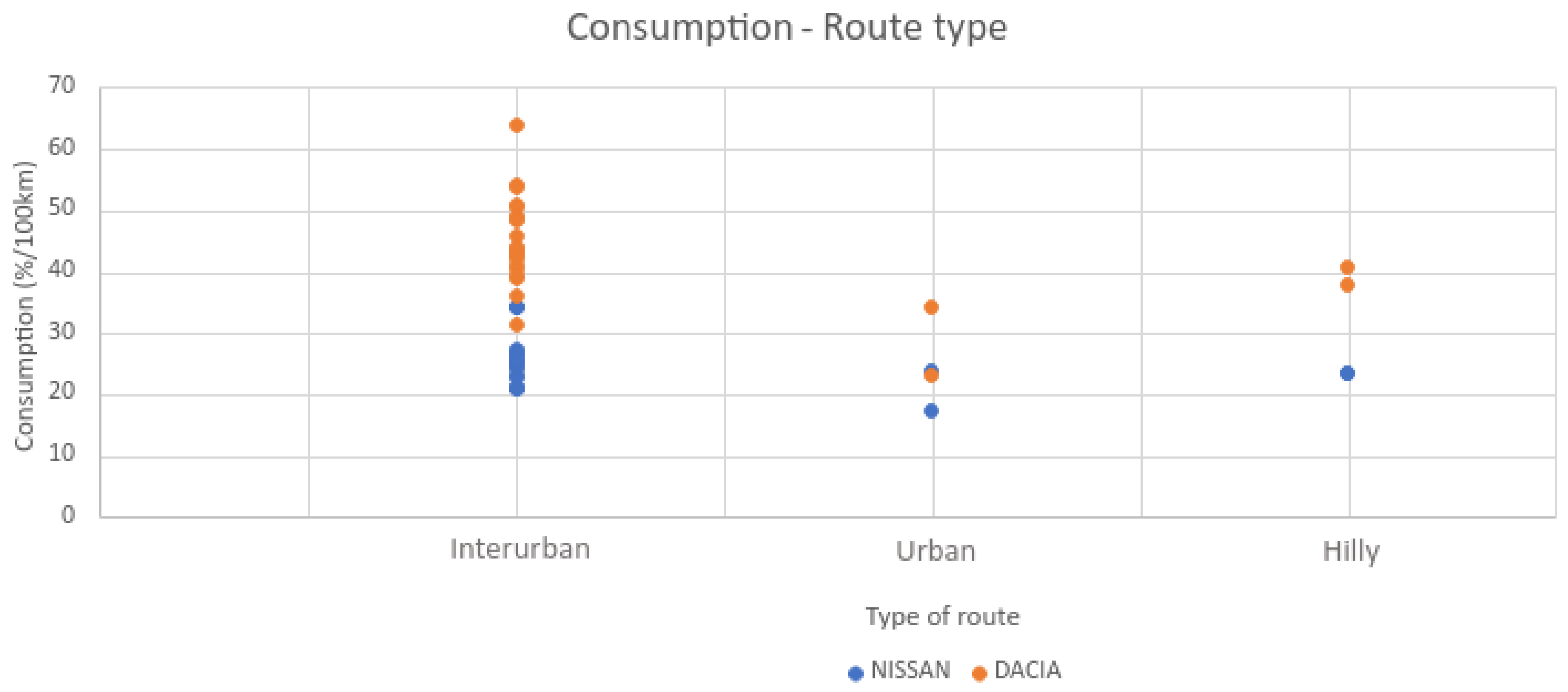
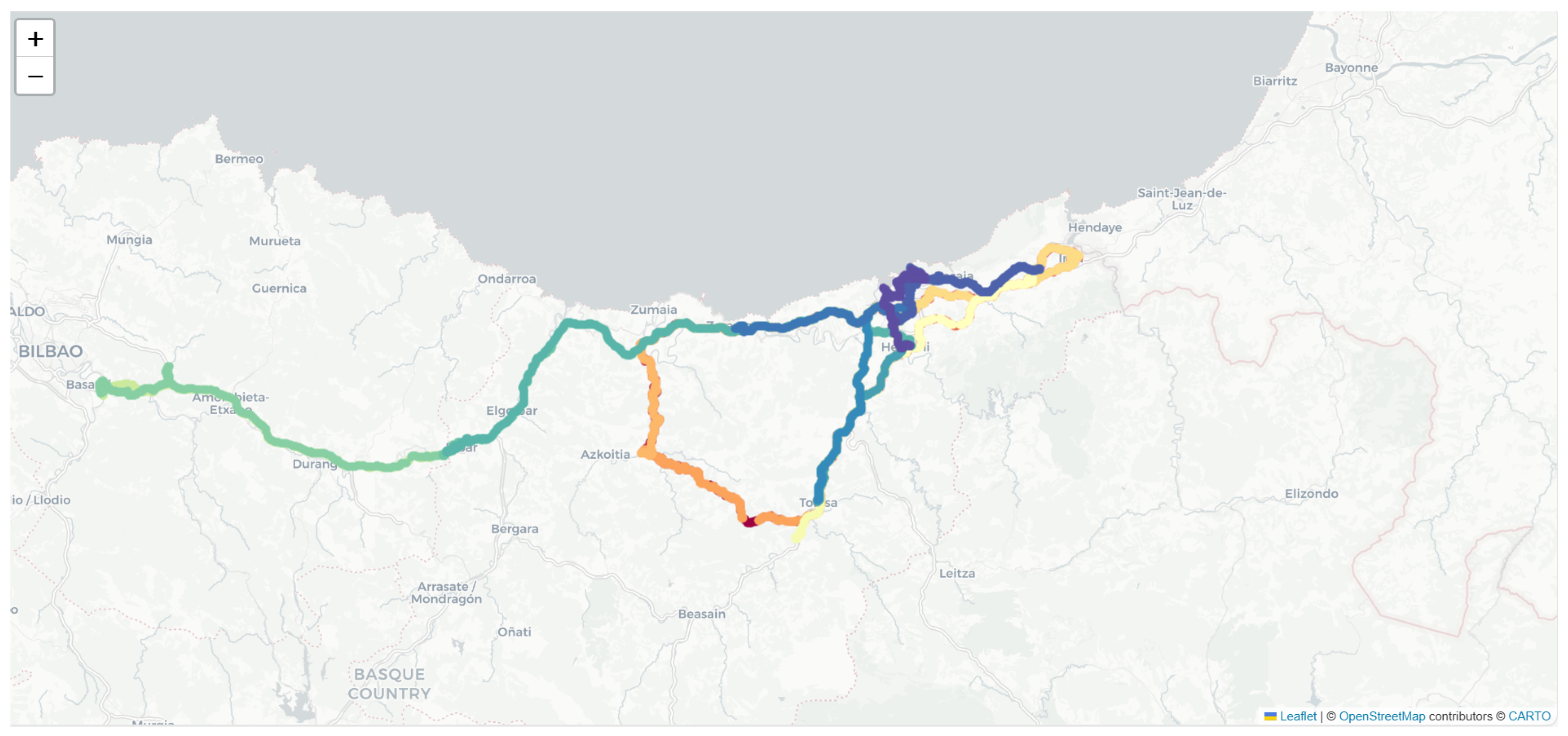
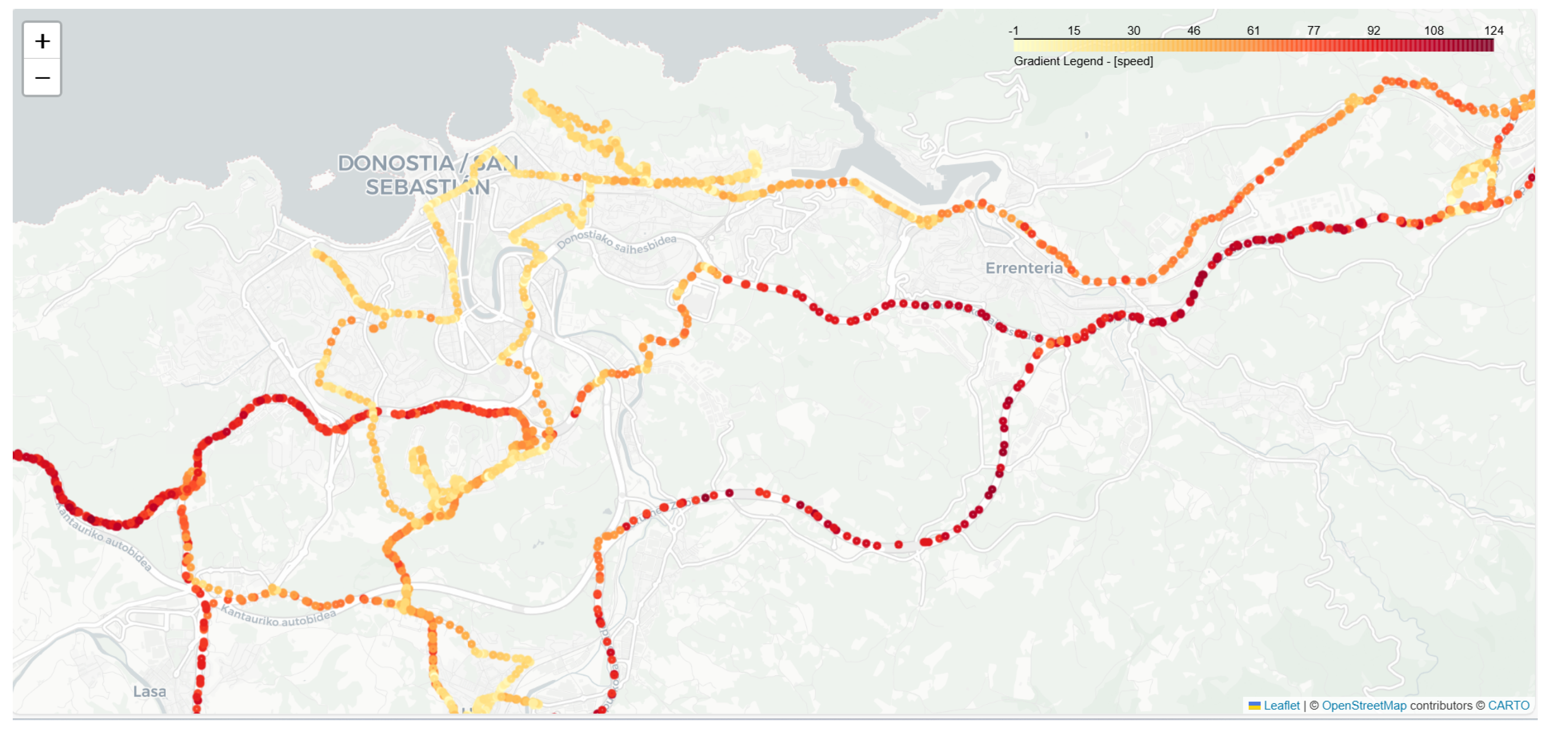
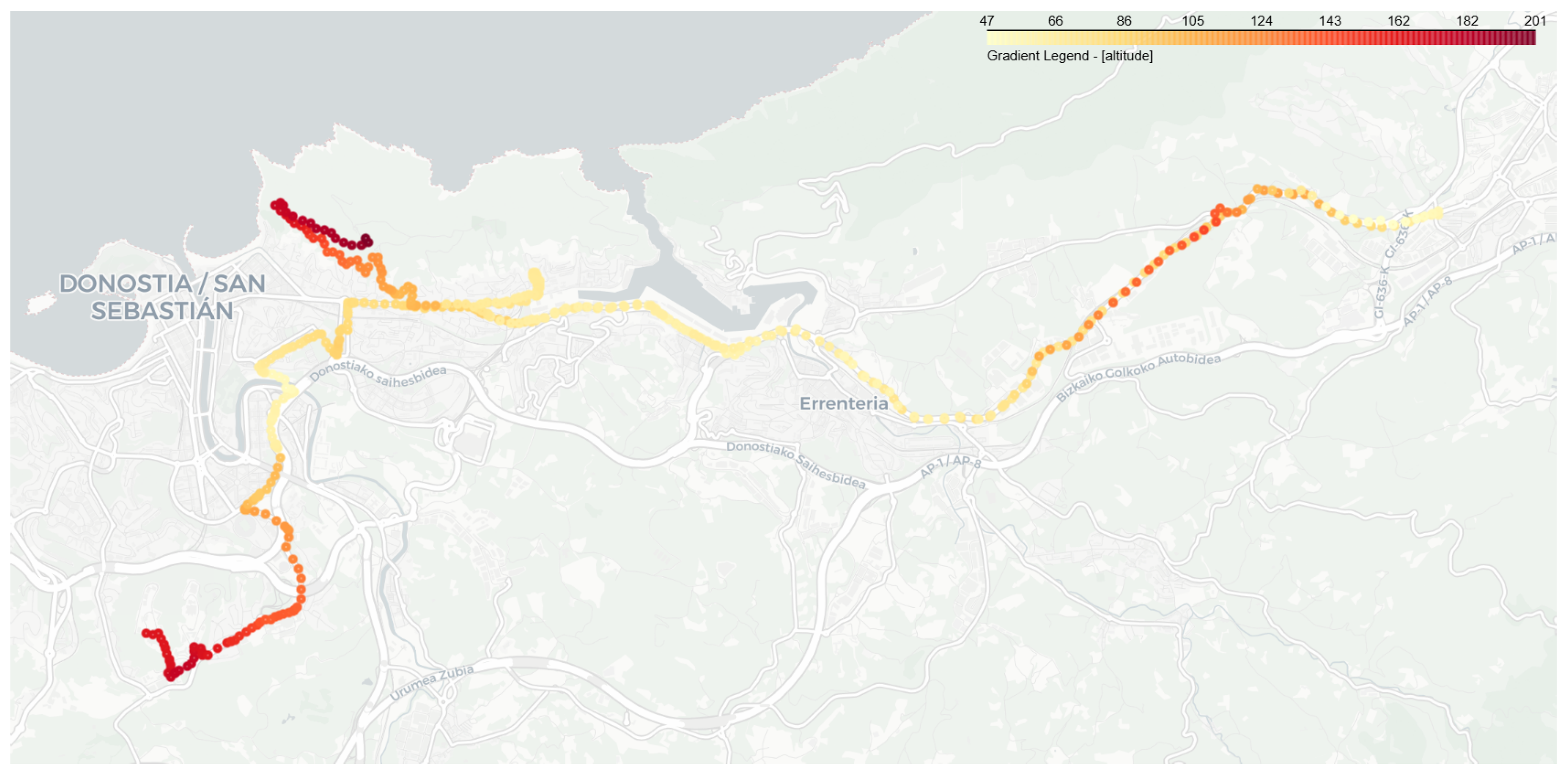
An overview of battery consumption values depending on the performed route type is depicted in Figure 1. The principal conclusion that can be obtained when analysing the data is that one of the vehicles performs better than the other on interurban and hilly roads, but on urban roads, the difference is not representative. It is shown, as well, that interurban routes are the most energy-demanding routes. The following maps represent the geographical distribution of the 58 tracks (Figure 2), the instantaneous vehicle speed measurements where different types of road categories can be distinguished from urban streets to highways (Figure 3), and how the elevation varies on one of the hilly routes (Figure 4). 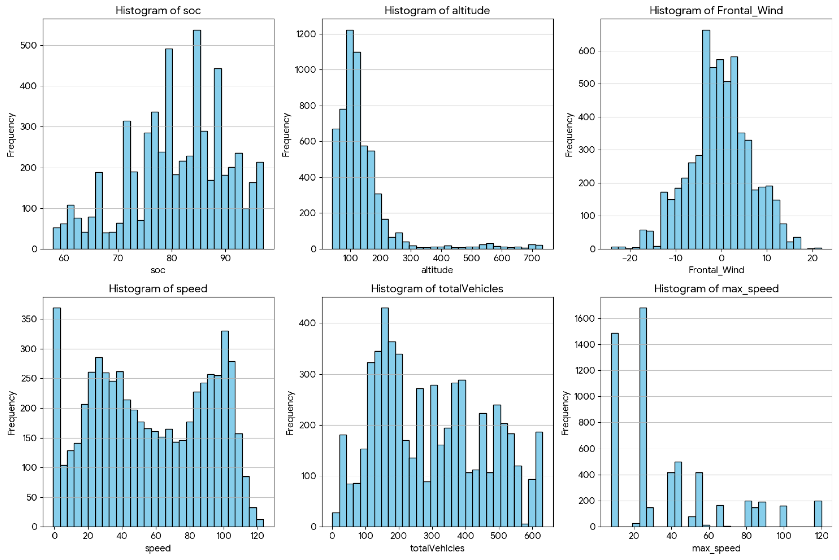Figure 5 depicts the statistical distributions of the SoC, altitude, frontal wind component, speed, traffic flow from the nearest counter and nominal maximum speed of the road network segments observed while performing different repetitions of the routes for Vehicles V1. A multi-modal distribution is observed for speed, with peaks representing urban driving (low speed) and highway segments (high speed), such that the maximum speed reached was 123.5 km/h. Traffic density shows a broad distribution, with a median of 264 vehicles, suggesting varying levels of traffic congestion during the data collection. The maximum speed reflects the legal speed limits of the roads travelled, with common thresholds at 10, 25, 55, and 120 km/h.

2.2. Heterogeneity and Completeness

The simultaneous use of two different vehicles raised some problems as well as opportunities. Since obtaining some OBD2 measurements from vehicles V1 was not possible during the data collection campaign, the use of a third party app was used. Speed measurements could not be extracted from vehicle V2, but aproximated data could be derived, as previously mentioned. Some differences were found, therefore, in the variables that are available in the dataset, depending on the vehicle. Nevertheless, since both vehicles were travelling together, but at a sufficient distance to avoid interference between them, variables such as ambient temperature or speed can be easily assumed. Both vehicles exhibit very similar mean maximum speeds, confirming that they were tested under comparable road conditions and speed limits. The mean altitude and maximum altitude are nearly identical across both datasets, ensuring that the impact of road gradient (slope) can be compared fairly between the two vehicle types. The traffic flow and frontal wind distributions are consistent between datasets, providing a controlled environmental baseline for cross-vehicle energy efficiency modelling.

The 5-day campaign was sufficient to observe heterogeneity of the traffic conditions in several routes, since they were repeated in multiple journeys including morning peaks vs. afternoon valleys.

3. Methods

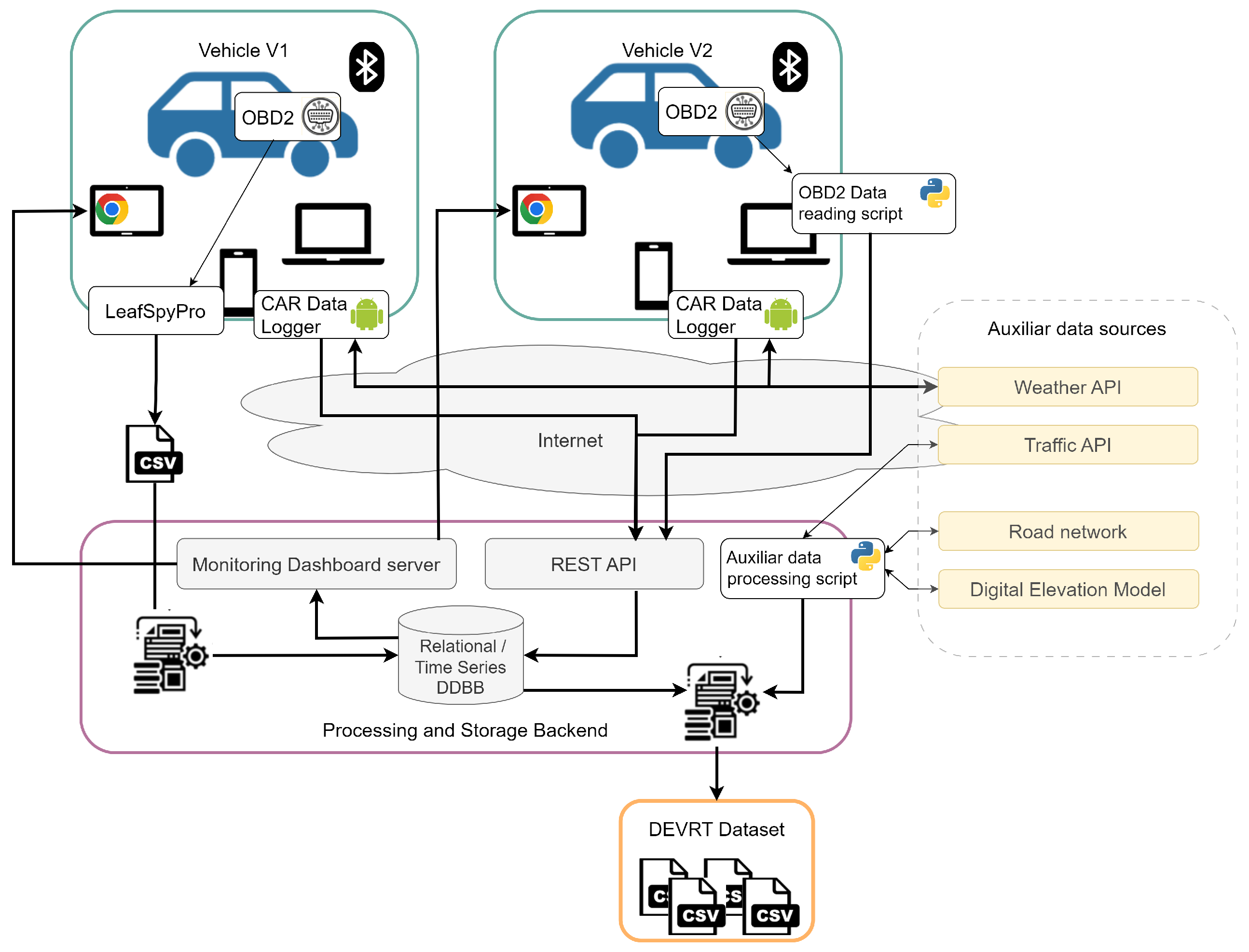
In this section, the devices and hardware/software toolsets and auxiliary datasets that were required in order to execute the multi-sensor data collection procedure and build the presented dataset are described. Then, the selected list of routes and the rationale behind this selection together with a detailed characterisation is given. Figure 6 represents a schematic description of all the tools and procedures flowchart.

3.1. Vehicles and Hardware

The following vehicles and hardware devices were used in the data-collection campaign.

3.1.1. Electric Vehicles

Two pure EVs were rented for a period of five consecutive working days, from Monday to Friday. The dates were scheduled two months in advance. The rental company provided some guidance about the category of vehicles that would be provided, but the final brand and models were known only one week before the start of the data collection, due to the varying availability of the vehicles.

Some electric vehicles in the market are more suitable for urban driving, while others are more suitable for highway settings and longer journeys. Each of the two vehicles provided by the rental company satisfied different purposes: a NISSAN LEAF™e+ 62 kWh (vehicle V1), intended for medium and long trips, and a DACIA SPRING™33 kW (vehicle V2), more oriented to urban usage. Therefore, two battery consumption variants were compared when performing different types of routes (urban, highway, big slopes, flat routes, etc.), not all of them for their intended use.

3.1.2. Electric Vehicle Chargers

Electric vehicles have different charger types. These differ in the charging technology and speed. The available types are Type 1, Type 2, Combo-type 2 (or CSS) and CHAdeMO. Type 1 supports single-phase AC charging up to 7.4 KW of power. Type 2 supports both single-phase and three-phase charging at higher power than type 1. CSS is an improved version of Type 2, compatible with AC and DC, up to 350 KW, and it is becoming mandatory in Europe. CHAdeMO supports DC charging up to 100 KW [23,24].

The supplied charging power and therefore the charging time required depend on the charging station, the connector type and the vehicle capacity. Both rented vehicle models worked with two connector types: vehicle V1 worked with Type 2 6.6 KW AC and CHAdeMO 46KW DC connectors, while vehicle V2 worked with Type 2 6.6 KW AC and CCS 34 KW DC [25].

3.1.3. OBD2 Devices

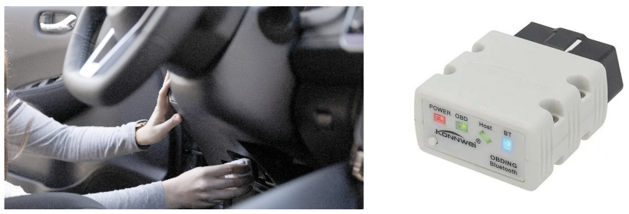
Vehicle telemetry was accessed via the On-Board Diagnostics (OBD2) interface using the Controller Area Network (CAN bus) protocol. Cars have multiple ECUs (Electronic Control Units), controlling one or more systems each. All the vehicle data go through the ECUs. Data retrieval was facilitated by two KONNWEI KW902 Mini Bluetooth adapters, manufactured by Shenzhen Jiawei Hengxin Technology Co., Ltd. from Shenzhen City, GD, China (Figure 7), which enable wireless connection, connect to Android and Windows PCs, and, according to the specifications and public online reviews, worked well for a variety of vehicle brands and models.

3.1.4. Laptops, Tablets and Smartphones

Each vehicle was equipped with a synchronized hardware suite comprising a smartphone, a laptop, and a tablet. Smartphones served as the primary gateway, capturing real-time GPS coordinates and atmospheric weather data while maintaining a Bluetooth link to the OBD2 adapter. They also acted as Wi-Fi hotspots for the onboard laptops. Laptops performed local data aggregation and facilitated transmission to the remote storage backend. Finally, tablets provided the drivers/researchers with a real-time monitoring dashboard to ensure data integrity during the trips.

All these hardware devices are presented in the general data collection architecture in Figure 6. In the next section, the data processing software installed in each hardware device is explained.

3.2. Software Tools

The hardware setup was very similar for both vehicles. Nevertheless, slight differences in the software setup were required due to specific particularities when extracting OBD2 measurements from each vehicle. Moreover, having several data sources added complexity to the data querying and post-processing. The complete architecture deployed to enable the data collection is depicted in Figure 6.

3.2.1. On-Board Data Processing Software

One of the main objectives of the software deployed on the hardware devices carried inside the vehicles is reading and processing meaningful data from the OBD2 ports, making use of codes known as electric vehicle Parameter IDs (PIDs).

Although some cars share some codes, especially those from the same manufacturer, every car model usually has its own specific codes. The biggest problem is that PIDs were not publicly available because manufacturers do not reveal them. The way to get to know them is to search in open repositories, specialised websites or forums in the Internet, namely collaborative work. Other alternatives are to discover the PIDs oneself using reverse engineering techniques or to use specific smartphone applications that connect to the OBD2 device and log car metrics. But this last option is limited to what parameters the application knows.

There are two types of PIDs, standard and non-standard or custom PIDs. Standard PIDs are parameters that are common and supported by almost every vehicle, for example, engine speed, throttle position, and fuel pressure. These are defined by the SAE J1979 standard [26].

Non-standard or custom PIDs are manufacturer-defined PIDs that are not defined in the OBD2 standard. For example, the SoC of an electric vehicle is one of these custom PIDs, but this information is very limited in the public domain. An example of the data needed for communicating with a Toyota Auris Hybrid can be seen in

Table 6. Data needed for communicating with the ECU of a vehicle.

Name	Mode and PID	Formula	Header
SoC	015B	A×20/51	7E2
MG1 Carrier Freq	217C	A/20	7E2
MG2 Carrier Freq	217C	B/20	7E2
…	…	…	…

.

The message to be sent to the ECU consists of the Header, the Mode, and the PID. Then, the ECU answers with another message that contains a value for the metric/metrics requested. Apart from knowing the query code, the response also has to be decoded with a specific formula. A standard response raw message from the ECU is depicted in Figure 8.

The processing pipeline starts with the OBD2 devices connected to the OBD2 ports and connecting to the OBD2 device via Bluetooth. Messages have to be sent to the ECUs to request for the specific vehicle parameters, but these messages vary from manufacturer to manufacturer and from vehicle model to vehicle model. Moreover, manufacturers do not reveal the specific codes of every parameter; therefore, it can be difficult to search and discover the needed PIDs (Parameter IDs) of any vehicle.

In this case, to query the data, different software has been used, depending on the vehicle. Although research on codes has been done over the internet and reverse-engineered with specialised software, the codes identified for vehicle V1 did not work, and a commercial alternative third-party software was used instead (the Leaf Spy Pro application). In the case of vehicle V2, the codes found were tested and worked properly. A python module was implemented based on the python-OBD library [27]. The laptop running this module queries vehicle data and sends it in real time to a developed API. The API stores all the data in a PostgreSQL database. The Leaf Spy Pro application, which could not send data to an external server, stored the collected information in CSV files in the memory, and they were processed afterwards.

An Android application was developed, Car DataLogger, and deployed in the smartphones in both vehicles to retrieve GPS positions, as well as weather data, and send them to the the remote server.

3.2.2. Remote Data Processing and Storage Backend

This remote data Processing and Storage Backend provides a REST API endpoint, a relational database, and a time-series database. It enables receiving information directly from the Android application in real time and allowing it to persist. Other modules developed for data querying and for processing the files extracted offline were a traffic information querying script and a wind effect calculation script. These two modules do not run in real time. They are used in post-processing once all the data files are received. Once every data source is stored and processed, a final round of data processing is executed to consolidate the different data sources and obtain the final dataset files. Details about the dataset are explained in Section 2.

3.2.3. Monitoring Dashboard

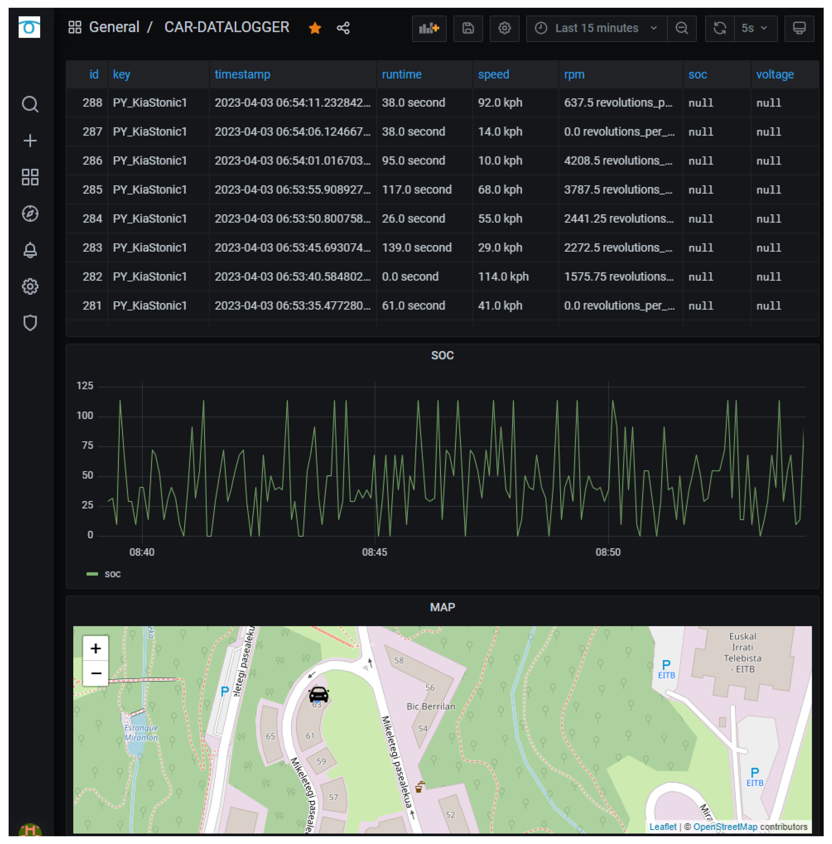
A dashboard was developed and deployed in the remote backend server in order to allow capabilities to monitor the metrics in real-time. This web-based dashboard was built with a visual charting framework and connected to the time-series database deployed in the remote back-end. The visualisation consisted of a map where vehicle position was represented, a table with weather information, a chart with SoC evolution, and another table with GPS data (Figure 9). During the driving tasks, the dashboard user interface was opened in the tablet web clients and supervised by the copilot, monitoring the situation in real time to ensure all data was being collected as planned.

3.3. Auxiliary Data Sources

Not every factor related to energy consumption can be extracted from the vehicle itself. There are other variables that affect the battery range, for example, the weather condition (ambient temperature, wind, rain, etc.), traffic situation, and road characteristics. This other data is also crucial but it must be obtained from external sources.

For the completion of this dataset, traffic and weather information have been obtained from external APIs and road network and elevation data sources.

3.3.1. Traffic Information

The trips were carried out within the Basque Country, Spain; therefore, traffic data provided by Basque Government Open Data Euskadi repository was exploited [28]. This API provides homogeneous count data from different roads, even if they are managed by different bodies: local, province or regional administrations. Data is aggregated in 30 min periods. Historical and real-time measurements are available, and both options are useful. However, for the sake of processing efficiency, traffic data was queried and added afterwards in post-processing, instead of during the driving tasks. The method selected was GET /v1.0/flows/byDate/year/month/day/byLocation/lat/lon/km, which provides categorised traffic counts aggregated every 30 min from the closest counter within a given radius, from a set of more than 12,000 counters across the region.

The output variables obtained from this dataset are the total number of vehicles, average speed, and number of vehicles categorised by speed and length. Some counters provide (0, 50, 80, 120, +) speed ranges, while others use (0, 80, 100, 120, +) and this depends on their configuration. Therefore, having consistent ranges across all locations was not possible.

3.3.2. Weather

Weather conditions affect battery performance, in particular, ambient temperature and wind. Although temperature affects battery range, this is a relevant factor only when considering extreme conditions, especially at low temperatures (below zero degrees Celsius). However, the resistance force a vehicle has to overcome often depends on the wind force and its direction, because the automobile’s drag is a force that acts parallel to and in the same direction as the airflow. Therefore, including wind-related measurements along with vehicle performance variables seems relevant to enable more exhaustive analysis of the EV battery consumption.

To collect wind data, a real-time weather data provider was selected: Weather API [29]. Data was requested from each vehicle using the smartphone, querying data every five minutes and referenced to its location at the moment. Among all the variables retrieved from this API, the ones added to the dataset were the ambient temperature, the wind speed (in miles per hour and in kilometres per hour), and the direction of the wind (reported in degrees and in cardinal or compass coordinates). It must be noted that the wind direction is reported as the orientation from which the wind is blowing.

The effect the wind has on each vehicle was simplified to its longitudinal effect. This frontal component of the wind is what most affects the vehicle’s battery consumption. A positive component means tailwind, which helpful to the vehicle’s travel, and a negative component means being against it.

3.3.3. Road Network and Elevation

The road network is represented as a graph, with nodes associated with approximate elevation values. OpenStreetmap [22] was the source selected to obtain the network and digital elevation models in HGT format [30] for the altitude information. The HGT file is map-matched to associate the nearest available elevation value from a data grid to each road network node. These auxiliary sources are of significant interest to characterise the type of road where the vehicles are driving, since OSM includes tags describing the category and speed limits of the road segments. Since not all road segments have this value included in the dataset (key = ‘max_speed’), when not available, theoretical speed limits have been assigned depending on the type of road indicated (key = ‘highway’). The elevation measurements enable further characterisation of the routes and their topology, as explained in Section 3.4.

3.4. Route Characterisation and Selection

Like internal combustion engine vehicles, the consumption of electric vehicles differs depending on the type of route. Speed and road slope are two factors that play an important role in electric battery consumption; therefore, significant differences can be found between urban, highway and mountain routes. The aim when selecting the routes was to diversify them as much as possible. This way, two vehicles intended for different purposes went on various types of routes, and specific analysis and conclusions can be extracted from this particularity.

3.4.1. Quantitative and Qualitative Characterisation of Routes

A route is defined as a sequence of route points that draw the journey from one origin to a destination. Being able to classify routes depending on their elevation profile helped the decision-making when developing a heterogeneous trip plan and ultimately analysing the impact on energy consumption of each type of route.

The reason is that EV battery consumption is affected by road gradient or slope. When driving on uphill gradients, the vehicle’s battery consumption tends to increase due to the extra power required to overcome gravity and maintain speed. Similarly, when driving downhill, the vehicle’s battery consumption may decrease or even become negative if regenerative braking is effectively utilised. On flat terrain, the energy consumption of an EV is typically more consistent and predictable compared to driving on varied gradients. However, factors such as speed, wind resistance, and traffic conditions still influence energy consumption.

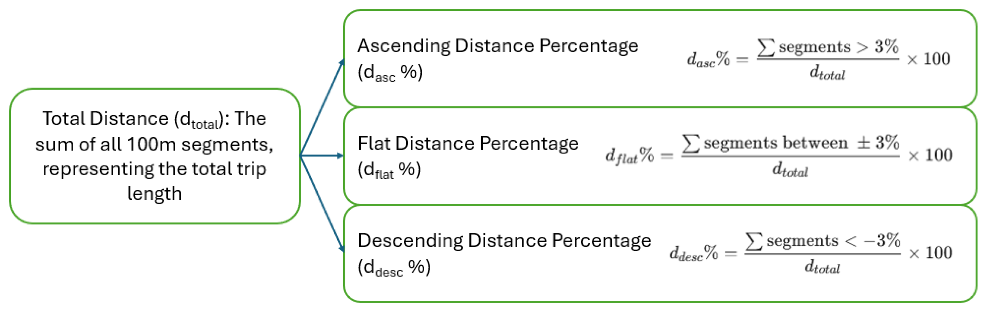
A method has been developed for route elevation profile characterisation, based on longitude, latitude and elevation data obtained from a trip. A trip is divided into segments of one hundred metres and the elevation difference is calculated in every segment of the route. If the slope is lower than −3%, the segment is classified as descending, if the slope is higher than 3% as ascending, and otherwise it is classified as flat. After multiple experiments were carried out, the segment distance and slope thresholds were the ones that best characterised different route elevation profiles. Figure 10 shows the technical description of the procedure. With this developed method, seven variables are created: distance, % of ascending distance, % of flat distance, % of descending distance, average ascending slope, average flat slope and average descending slope.

3.4.2. Features of Interest and Eligibility of Routes

The motivation for evaluating a set of distinct route types was that they affect electric vehicles in different ways.

In the case of urban routes, speeds are lower, which makes battery range larger, and there are many idling moments when waiting for traffic lights without an adverse effect [31]. These conditions are also present in traffic congestion situations. Furthermore, every EV has capabilities for regenerative braking, an action that is often found in urban driving.

The nature of highway driving is significantly different. Speeds are higher and have a major impact on battery performance. Usually, meaningful traffic congestion situations happen less often, and although regenerative braking is also used, its impact on the overall energy consumption is small. Some features that have a greater impact than in urban driving are weather conditions and driving style. For instance, as speeds are higher, wind can provoke a higher resistant force on the vehicle to keep the desired pace. This translates into a higher energy consumption. At the same time, aggressive or non-moderate driving with many acceleration changes or at very high speeds will shorten the battery range. Finally, mountain roads are known for having significant slopes and elevation changes. In the case of going upwards, the vehicle requires more energy, but in the case of going downwards, a significant part of the energy can be recovered due to regenerative braking.

The susceptibility of electric battery performance to such circumstances makes considering different route types important.

3.4.3. List of Final Routes

The list of performed routes and each one’s elevation characterisation is detailed in

Table 7. Slope characterisation of the routes taken.

O-D	Type	Length (km)	% Asc.	% Flat	% Desc.	Avg. Slope Asc.	Avg. Slope Flat.	Avg. Slope Desc.
R1: Andoain–Azpeitia	hilly	34.2	26.0	44.1	27.6	7.8	0.2	−7.6
R2: Azpeitia–Donostia	interurban	43.4	25.1	53.2	20.5	4.4	−0.1	−4.8
R3: Donostia–Hernani	urban	4.2	2.5	55.2	36.3	8.1	0.3	−6.2
R4: Donostia–Irun	interurban	28.6	17.2	63.1	17.3	4.6	−0.0	−5.2
R5: Hernani–Tolosa	interurban	18.6	13.5	74.2	10.2	5.0	0.1	−5.0
R6: Irun–Andoain	interurban	23.5	14.8	61.5	22.5	4.4	0.2	−3.8
R7: Tolosa–Zarautz	interurban	33.0	14.0	68.7	16.3	4.7	0.0	−5.0
R8: Zarautz–Donostia	interurban	20.3	32.3	47.3	19.4	5.2	−0.1	−6.0
R9: Donostia–Tolosa	interurban	21.8	6.9	78.4	12.6	5.5	0.3	−6.9
R10: Tolosa–Donostia	interurban	27.3	6.7	87.9	4.1	5.7	−0.1	−3.6
R11: Bilbao-Eibar	interurban	38.5	6.4	86.0	6.7	4.3	0.2	−5.0
R12: Eibar–Bilbao	interurban	41.0	9.7	77.7	11.1	6.8	−0.2	−5.3
R13: Eibar–Donostia	interurban	56.9	15.6	65.5	17.9	6.7	−0.1	−5.4
R14: Hernani–Eibar	interurban	58.7	19.6	61.9	17.0	4.7	0.3	−5.8
R15: Donostia–Ulia	urban	37.8	19.2	56.3	19.0	6.2	0.0	−6.1
R16: Ulia–Hernani	urban, hilly	17.3	26.3	34.1	33.6	8.4	0.2	−8.7

. Some differences and similarities can be extracted from the characterisation data. Hilly routes are those with a higher percentage of ascending/descending distance and higher slope values. Interurban routes are mostly flat, although there could be some road sections with a considerable slope. In the case of urban routes, there is a mix of values because of the specific orography of the municipality. One of the routes (R3) is shorter than the others. This route was the distance from the research team laboratory to the nearest public charging point, used as a reference point to many other routes.

3.5. Data Collection Procedure

Four researchers were involved in the data collection, and one additional researcher checked the proper functioning of the monitoring dashboards remotely. With two researchers in each vehicle, all the routes were driven simultaneously by the two vehicles. Each pair always drove the same vehicle, but driver and assistant roles were exchanged. Thus, the traffic and weather conditions were exactly the same.

The data collection procedure was a big challenge for many reasons. Although it was known that one vehicle would be more intended for long-distance routes and the other one for urban ones, the brand and model of the two rented vehicles were notified by the rental company only one week before the start of the renting period. This added uncertainty to whether the researched PIDs would work or not. In case they did not work, the preparation involved researching alternative PIDs, reverse-engineering software for parameter discovery, and third-party applications for ECU data listening. Another challenge was the limited amount of time available for travelling all the proposed routes, taking into account that some unexpected issues could arise, for example, the possibility of losing GPS and internet connection in mountain routes, or the immature level of charging infrastructure, with very few chargers in some areas. Regarding the charging infrastructure, it was decided to split the routes into shorter distances between charging stations and to always have a comfort battery level remaining to prevent the situation of arriving with low battery to a charger and realising that it was not operative, as happened once.

3.5.1. Daily Schedule

Taking into account the selected routes and the time needed to accomplish them, a plan was made for the five consecutive days.

On Day 1, the vehicles were picked up first thing in the morning. During the morning all the software connections were made, the PIDs and the retrieved data were tested. In the afternoon, some charging operations were done in different charging operators to test the charging applications, the connectors and the charging speed. This way, everything was prepared to start making the trips the next day. Days 2 and 3 were planned to drive some specific interurban routes more than once. The rationale behind repeating routes was that there could be different driving style, traffic and weather conditions. On Day 4, a round trip of a longer interurban route was driven. Finally, on Day 5, urban routes were carried out and the vehicles were returned to the rental company. The daily activities and charging activity are summarised in

Table 8. Summary of the daily schedule.

Day	Main Purpose	Charging History (min, kWh)	Incidents
Day 1	Pickup and familiarisation with vehicles. HW and SW connectivity and PID tests. Test chargers and charging applications	(1, 0.16); (25, 8.12)	Problems to read SoC (V1) and speed (V2)
Day 2	Interurban routes	(43, 17.46); (52, 24.91); (56, 6.30); (53, 5.68); (8, 5.99); (26, 9.26)	-
Day 3	Interurban routes	(28, 14.98); (40, 15.89); (48, 5.09); (48, 5.39); (7, 0); (3, 0.09); (53, 18.31)	Charger not working
Day 4	Round trip for a long interurban route	(5, 3.61); (34, 11.69); (26, 17.02); (26, 8.51); (31, 6.90); (107, 10.80); (7, 2.00); (29, 9.92)	-
Day 5	Urban routes and delivery of vehicles to the rental office	(22, 6.25)	-

. It must be noted that the charging speeds differed significantly due to the variations between the different charging stations.

3.5.2. Preparation

The hardware and software preparation procedures were similar for both vehicles. Before the beginning of the rental period, the scripts required for querying data were prepared. Once the two cars were brought from the rental office to our research facilities, connections with all the devices had to be made and tested. The first objective was to find the OBD2 port and connect the device, as seen in Figure 7. In some vehicle models, the OBD2 port is not visible or directly accessible and it requires removing a cover. In the Dacia Spring, a laptop was connected via Bluetooth to the OBD2 device, and a smartphone shared internet connection to the laptop at the same time that weather data was queried. In the Nissan Leaf, the same smartphone that queried weather data was the one connected via Bluetooth to the OBD2 device, and it retrieved metrics through the Leaf Spy Pro application.

In order to avoid auxiliary power consumption from the vehicles that would distort SoC measurements, preparation also involved fully charging the batteries of laptop, tablet and smartphones overnight to be ready in the morning.

3.5.3. On-Route

Each car was occupied by a primary driver and a technical assistant as already mentioned. The assistant was in charge of starting the whole data collection procedure and monitoring it in real time through the monitoring dashboard in a tablet. This continuous oversight enabled immediate detection and mitigation of potential data loss or connectivity interruptions. Given that certain EV interfaces provide only coarse SoC estimations (e.g., level bar or an estimation of remaining range in kilometres), the monitoring dashboard provided high-fidelity, granular SoC percentages retrieved directly from the vehicle’s internal metrics. This centralized interface allowed for inter-vehicle coordination, since both car assistants were in constant communication and monitoring both vehicles metrics through the same dashboard simultaneously. In addition, another person supervised the data collection remotely to ensure data integrity across the fleet.

3.5.4. Post-Processing

Upon completion of each day’s tracks, a preliminary validation of all collected data was performed, confirming their completeness, followed by the execution of a comprehensive database backup to ensure data persistence and redundancy. The final post-processing at the end of the data collection week involved adding extra information (traffic) and carrying out specific calculations (frontal wind effect).

Traffic data integration was performed using an iterative spatial query. For each vehicle coordinate, the API was queried within an initial radius of 1 km; this search radius was incremented in 1 km steps until a monitoring station was identified. Consequently, larger radius values indicate a lower spatial density of sensors relative to the vehicle’s trajectory, and the relevance of the traffic information may be lower, potentially representing traffic from other roads.

The methodology for integrating frontal wind effects is structured as follows: During post-processing, the vehicle’s heading is defined by a displacement vector calculated between consecutive GPS coordinates. These vehicle trajectories are then temporally aligned with the most proximal wind data points. Given that meteorological wind direction is conventionally reported in degrees clockwise from North (0 degrees), while the Cartesian system defines North at 90 degrees with counter-clockwise rotation, a coordinate transformation is required. This conversion is a prerequisite for decomposing the wind vector into its longitudinal component relative to the vehicle’s path. After transforming both vectors into a unified coordinate system, the longitudinal wind component is derived from the cosine of the relative angle between the vehicle and wind vectors. By convention, a negative result denotes a headwind (opposing motion), while a positive result indicates a tailwind (aligned with motion).

Finally, the data from both vehicles is standardized to ensure a consistent format.

4. Usage Notes

The dataset includes a supplementary python script usage_example_DEVRT.py, which includes functions and examples for loading, describing the CSV files and plotting the tracks in a map.

The described work presents some limitations that are worth noting.

• The differences in the data-collection procedure for the two vehicle models limited the homogeneity of the dataset. For instance, it lacks the instantaneous speed for one of the vehicles.
• The dataset covers a relatively limited temporal extension (5 working days) and mileage, given the availability of the two vehicles that were rented.
• Due to the difficulty of knowing the exact vehicle PIDs and the limited time to test the researched ones, although the SoC and SoH of V2 could be retrieved, the PID for the speed did not work, and the dataset lacks this metric. However, the dataset has timestamp and latitude/longitude data, so calculating an average speed between desired segments is possible.
• A simplification was made to calculate only the longitudinal wind effect on the vehicle. The authors consider this longitudinal component as the most important one, acknowledging that the transversal wind force also affects electric battery performance, but to a lesser extent. Moreover, vehicle direction is simplified to the vector that is formed from consecutive time steps. For the full wind effect in electric vehicle battery performance calculation, the vehicle should be equipped with additional sensors to register instantaneous vehicle direction and wind metrics.
• Regarding traffic data, road conditions can vary depending on events like accidents, roadwork, traffic light malfunctioning, etc. Even on the same road, there could be segments with different traffic conditions, and traffic counters may not be measuring those specific segments. Traffic data obtained for this dataset has been queried from the closest meter within the smallest radius available. This can lead to having data from a road that do not corresponds exactly with the road that the vehicle is in, but overall, it provides comparable traffic condition from the closest measured point.
• The type of charging station used to charge the vehicle each time was not annotated. This information would have helped to explain the variations in the charging speeds.
• The scope of the work was not able to include observing and understanding user behaviour and preferences relative to electric vehicle movement. These are crucial for predicting and shaping electric vehicle movement patterns. Factors such as trip purposes, travel patterns, charging habits, and vehicle preferences influence how EVs are utilised and integrated into daily transportation routines. The study has been limited to deliberately selected journeys with researchers participating as drivers during the data collection.

The dataset is to be complemented and improved in future data-collection campaigns, addressing most of the identified limitations. Future plans in this regard envision longer campaigns (2–3 weeks) to increase the variety in weather and traffic situations, maintaining the decision of using two simultaneously driven vehicles. In spite of these limitations, the methodology and toolset presented can be extrapolated and applied by researchers and practitioners into different vehicle fleets driven by diverse research subjects so that their data can be collated during longer data collection campaigns and, at the same time, their behaviour and preferences can be explored. The current published dataset consists of real-world data records of two vehicle models that are currently in the EV market, in a context where brands and models evolve very fast. Moreover, the lessons learnt open future work towards the collection of data from other kinds of vehicles such as electric motorbikes and bikes.