Article

Development of Artificial Neural Network Models to Assess Beer Acceptability Based on Sensory Properties Using a Robotic Pourer: A Comparative Model Approach to Achieve an Artificial Intelligence System

by
Claudia Gonzalez Viejo
*,
Damir D. Torrico
,
Frank R. Dunshea
and
Sigfredo Fuentes
School of Agriculture and Food, Faculty of Veterinary and Agricultural Sciences, University of Melbourne, Parkville, VIC 3010, Australia
*
Author to whom correspondence should be addressed.
Beverages 2019, 5(2), 33; https://doi.org/10.3390/beverages5020033
Submission received: 6 March 2019 / Revised: 29 March 2019 / Accepted: 9 April 2019 / Published: 1 May 2019
(This article belongs to the Special Issue Brewing and Craft Beer)

Abstract

:
Artificial neural networks (ANN) have become popular for optimization and prediction of parameters in foods, beverages, agriculture and medicine. For brewing, they have been explored to develop rapid methods to assess product quality and acceptability. Different beers (N = 17) were analyzed in triplicates using a robotic pourer, RoboBEER (University of Melbourne, Melbourne, Australia), to assess 15 color and foam-related parameters using computer-vision. Those samples were tested using sensory analysis for acceptability of carbonation mouthfeel, bitterness, flavor and overall liking with 30 consumers using a 9-point hedonic scale. ANN models were developed using 17 different training algorithms with 15 color and foam-related parameters as inputs and liking of four descriptors obtained from consumers as targets. Each algorithm was tested using five, seven and ten neurons and compared to select the best model based on correlation coefficients, slope and performance (mean squared error (MSE). Bayesian Regularization algorithm with seven neurons presented the best correlation (R = 0.98) and highest performance (MSE = 0.03) with no overfitting. These models may be used as a cost-effective method for fast-screening of beers during processing to assess acceptability more efficiently. The use of RoboBEER, computer-vision algorithms and ANN will allow the implementation of an artificial intelligence system for the brewing industry to assess its effectiveness.

1. Introduction

Machine learning is defined as the computer-based system that is able to learn and find patterns among the data to predict specific outputs [1,2]. There are different types of machine learning from which two main categories are derived: (i) pattern recognition or classification and (ii) fitting or regression [3]. The first is mainly used for decision making as it classifies samples into two or more categories, the most publicized applications can be found in medical diagnosis [4,5], food and beverages to classify into types of brewages [6,7,8] and level of liking of brewages [8,9], in agriculture for identification of grapevine cultivars [10], and to estimate plant water status [11], among others. Fitting or regression is used to predict specific values of certain variables such as chemical compounds [7,12], sensory descriptors [13], and microbial spoilage [14] among others.
There are different types of regression algorithms, which can be classified within categories such as linear regression, regression trees, support vector machines, Gaussian process, ensemble of trees and artificial neural networks (ANN) [15]. The latter has been widely used due to its non-linearity and ability to find patterns from inputs in a similar way to the functioning of neurons in the human brain. These algorithms are able to learn from data by testing and modifying weights and biases until they find the best correlation [7,16]. Furthermore, it has the advantage that the derived ideal relationship, which links the inputs and outputs, is obtained during the training stage [17,18]. There are several ANN training algorithms that may be used, which can be classified into four main categories: (i) backpropagation with Jacobian derivatives, (ii) backpropagation with gradient derivatives [3], (iii) supervised weight and bias, and (iv) unsupervised weight and bias training functions [19]. In this paper, only the first three categories will be used.
The use of machine learning algorithms, especially ANN, in food and brewages has become more popular in recent years as they aid in the increase in accuracy, time and cost reduction in analytical and sensory methods to assess quality and acceptability of beverages [20]. Specifically, in beer, it has been used in the prediction of chemical compounds using near-infrared spectroscopy [7,21,22], and prediction of the intensity of sensory descriptors [13,23].
This paper aimed to find the best machine learning regression model by comparing 17 different ANN training algorithms to predict the liking of four sensory attributes of beer using 15 color and foam-related parameters measured using a robotic pourer (RoboBEER), and computer vision algorithms [6]. For this purpose, 17 beer samples from different styles and from the three types of fermentation (top, bottom and spontaneous) were analyzed in triplicates to develop the models. The targets considered for the models were obtained conducting a sensory session with 30 consumers which rated the liking of four attributes (carbonation mouthfeel, bitter taste, flavor and overall liking). After comparing the models developed using the 17 training algorithms, the best model was selected on the basis of best performance. The best models found may potentially be used for fast-screening of beer samples in product development and/or at the end of the production line to assess beer acceptability without the need of recruiting consumers, which is more cost-effective and less time-consuming.

2. Materials and Methods

2.1. Beer Samples Description

Triplicates of 17 different beer samples (N = 51) from different countries, styles and type of fermentation (Table 1) were used to assess their color and foam-related parameters. However, only one replicate was used to assess consumer acceptability as the replicates were obtained from bottles belonging to the same production batch.

2.2. Color and Foam-Related Parameters

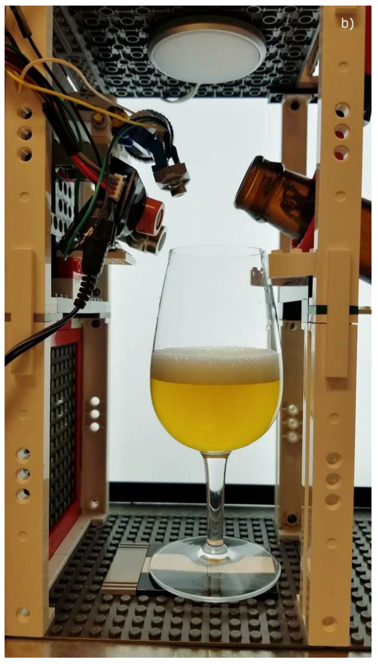
Color and foam-related parameters were obtained using a robotic pourer, RoboBEER (University of Melbourne, Melbourne, Australia), to ensure uniform pouring. RoboBEER works with two Lego® servo motors and has three sensors attached that work with Arduino® (Arduino, Ivrea, Italy): (i) temperature, (ii) alcohol and (iii) carbon dioxide (CO2) gas release and is coupled with an iPhone 5S to record 5 min videos of the pouring (Figure 1). These videos were then analyzed with Matlab® R2018b (Mathworks Inc., Matick, MA, USA) using customized computer vision algorithms. The first algorithm worked in a semi-automatic way, which consisted of standardizing and scaling the glass size by selecting the height and glass rim in the first frame of the video, followed by the manual selection of the foam height every 30 frames for the algorithm to automatically calculate the foam and beer volume. These results were then used to develop the foam volume versus time curve and to calculate the following parameters: (i) maximum volume of foam (MVol), (ii) total lifetime of foam (TLTF), (iii) lifetime of foam (LTF), and (iv) foam drainage (FDrain). Furthermore, a single frame of the video (highest in foam) was processed using other algorithms in Matlab® to assess color in two scales CIELab [(v) L, (vi) a, (vii) b] and RGB [(viii) R, (ix) G, (x) B] as well as bubble size distribution divided in (xi) small (SmB), (xii) medium (MedB), and (xiii) large bubbles (LgB), the latter were analyzed based on the “Hough Transformation” from the middle section of the foam and classifying bubble size based on the diameter measured in pixels. Additionally, the parameters (xiv) alcohol (OH) and (xv) CO2 gas release from the sensors were obtained. More details about the robotic pourer and computer vision analysis can be found in the paper from Gonzalez Viejo et al. [6]. All data were analyzed using customized codes in Matlab® and a Titan Xp GPU (NVIDIA Corporation, Santa Clara, CA, USA).

2.3. Sensory Session

A double-blind sensory session to assess beer acceptability was conducted with 30 consumers using a 9-point hedonic scale. According to the Power analysis, this sample size of consumers is enough to compare samples in a sensory test (1–β > 0.99). The session was conducted in individual booths with uniform lighting located in the sensory laboratory of the Faculty of Veterinary and Agricultural Sciences of The University of Melbourne. Before the sensory session, participants were asked to sign a consent form in accordance with the ethics approval 1545786.2 by the Human Ethics Advisory Group (HEAG) of the Faculty of Veterinary and Agricultural Science at The University of Melbourne. The beer samples were semi-randomized in two blocks of eight and nine samples at refrigeration temperature (4 °C) and participants were provided with crackers and water to cleanse the palate and to allow them to rest between samples to avoid fatigue. The sensory attributes evaluated and used as targets for the model construction consisted of (i) carbonation mouthfeel (MCarb), (ii) bitter taste (TBitt), (iii) flavor, and (iv) overall liking (overall).

2.4. Machine Learning Modelling

Seventeen training algorithms (Table 2) were used to develop artificial neural network models using a customized Matlab® code capable of testing all the algorithms in a loop. The models were developed using as inputs the normalized values (from −1 to 1) of the 15 color and foam-related parameters measured with the RoboBEER: (i) MVol, (ii) TLTF, (iii) LTF, (iv) FDrain, (v) L, (vi) a, (vii) b, (viii) R, (ix) G, (x) B, (xi) SmB, (xii) MedB, (xiii) LgB, (xiv) OH and (xv) CO2, and the four sensory attributes as targets/outputs: (i) MCarb, (ii) TBitt, (iii) flavor, and (iv) overall.
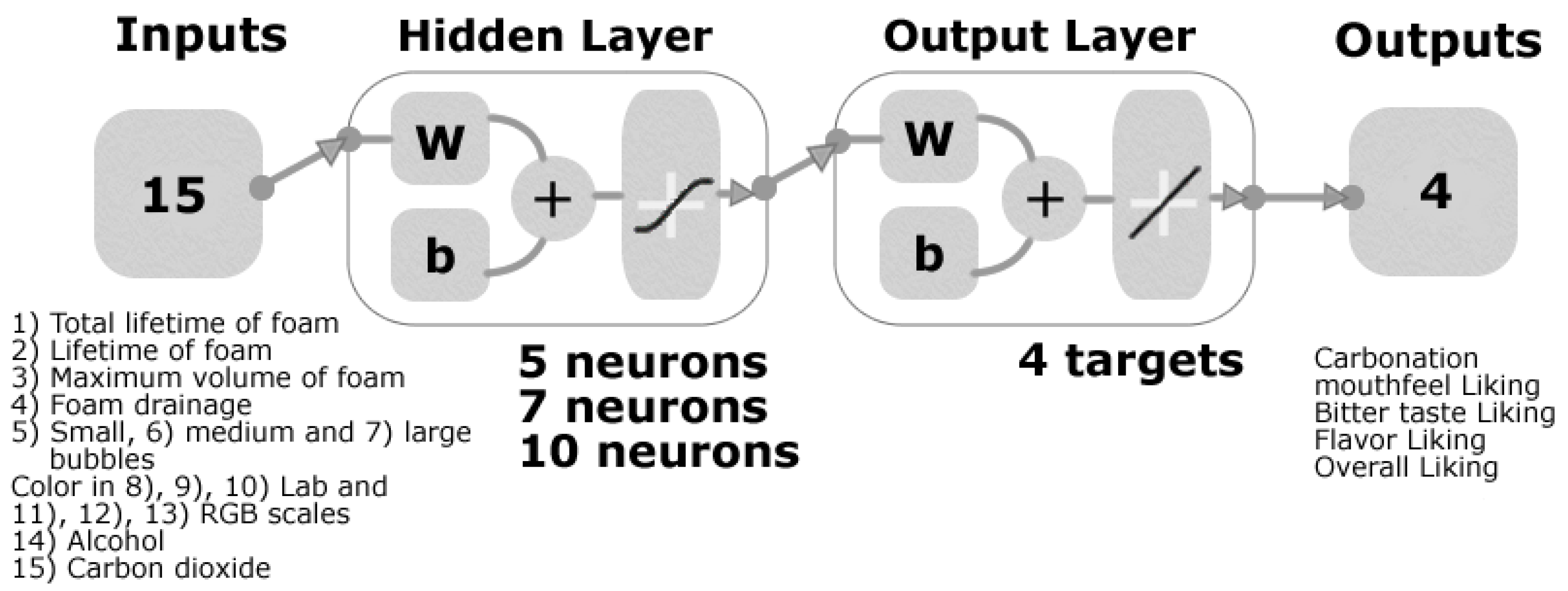
A neuron trimming exercise (5, 7 and 10 neurons) was performed for each algorithm. Ten was the largest number of neurons tested as using fewer neurons and obtaining good models without overfitting is the best practice. Using a larger number of neurons would most likely lead to overfitting. All models were developed using a random data division considering 70% (n = 35) of samples used for training, 15% (n = 8) for validation using a mean squared error performance algorithm, and 15% (n = 8) for the testing stage with a default derivative function. The models were constructed based on a two-layer feedforward network with a tan-sigmoid function in the hidden layer and a linear transfer function in the output layer (Figure 2).
The statistical analysis to evaluate and compare the accuracy of the models developed consisted of the correlation coefficient (R), determination coefficient (R2), mean squared error (MSE) to assess performance and slope (b) for each stage (i) training, (ii) validation, (iii) testing, and (iv) overall model as well as the p-value for the overall model. For the three best models, the percentage of outliers using 95% confidence bounds were obtained.

3. Results

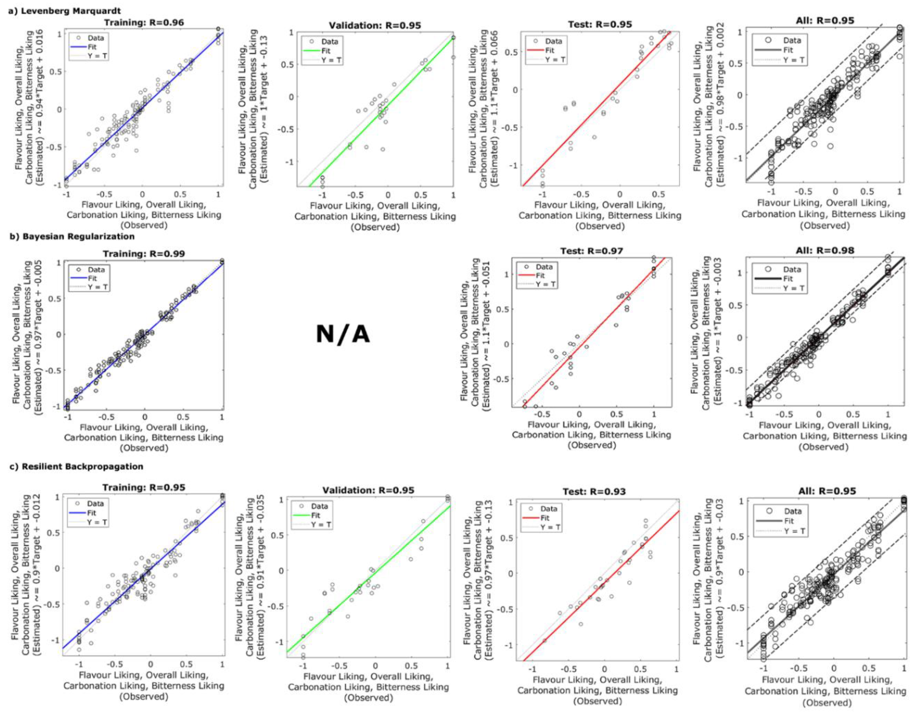
Table 3 shows the statistical data of the best and worse models developed from each group of training algorithms. For the backpropagation with Jacobian derivatives algorithm, there was no worse model as those from both algorithms within the group produced two of the best models. Tables S1–S3 in Supplementary Material show the statistical data of the models developed using the 17 training algorithms. Correlations from all models were significant with a p-value < 0.0001. It can be observed that the algorithms with the lowest R and R2 were from the gradient descent backpropagation with five and seven neurons (Table 3; Table S1), the batch training with weight and bias learning rate with seven neurons (Table 3) and the sequential order weight and bias with five neurons (Table S3). On the other hand, the models with the highest R and R2 were with those developed using seven neurons from both algorithms belonging to the backpropagation with Jacobian derivatives function (LM and BR) and the RPROP with R values consistently over 0.90 for all stages (Table 3). Furthermore, the slope from these three best models was close to unity (b ~ 1) for all stages, with the RPROP having the lowest slope values with a b = 0.90 for the overall model (Table 3; Figure 3). On the other hand, the three models had low MSE values (≤0.06) for the three stages and overall model. Table 3 also shows the best model from the supervised weight and bias algorithms; however, this still had some signs of overfitting as the validation and testing performances were not as close (MSE = 0.10 and 0.06, respectively) and the R values were lower than the three best models.
Figure 3 shows the training, validation, testing and overall models of the three best algorithms developed using 7 neurons. Model 1 (Figure 3a), which was developed with the Levenberg-Marquardt algorithm, had a training R = 0.96, and validation, testing and overall R = 0.95, furthermore, the overall model had 6.86% of outliers according to the 95% confidence bounds. Figure 3b shows Model 2 with the Bayesian regularization algorithm with R = 0.99 for the training stage, R = 0.98 for testing and overall model with R = 0.98 and 5.88% outliers, this algorithm does not use a validation stage. On the other hand, Figure 3c depicts Model 3 developed using the RPROP algorithm, which also had a high R = 0.95 for training and validation stages, R = 0.93 for testing and an overall model with R = 0.95 and a low percentage of outliers (4.90%). It can be observed that in the overall models, some predicted values are >1 or < −1, this is because the targets were normalized based on the range of data obtained in the study (3–7); however, the liking hedonic scale is within the 1–9 range, therefore, a value <−1 or >1, will still fit within the 1–9 scale when reversing the normalization.

4. Discussion

According to Beale, et al. [24], an indicator of a good model with no overfitting is when the validation correlation coefficient is close to the value from the training stage, which was met by the three best models found in this paper (Table 3 and Figure 3). The Bayesian regularization model (Model 2) does not have a validation stage; however, the R values of the other three stages are high and similar. Furthermore, an indication of a model with no overfitting is that the training performance (MSE) must be lower than the other stages, and the gap between the validation and testing MSE must be small [3,24]. This was also met by the best models found in this paper (Table 3).
The Levenberg-Marquardt algorithm (Model 1) is a backpropagation function, which works by calculating the second derivatives of a cost function. The advantages of this algorithm are: (i) that it is capable of giving a solution even though its start-point is far from the final minimum, (ii) its processing time is one of the lowest compared to other algorithms, (iii) the training algorithm stops when it finds the maximum epoch and (iv) the best performance value is achieved, or when it finds that the gradient value is lower than its minimum [25]. However, some disadvantages include: (i) it may not always secure a global optimum for an unrestrained optimization issue and ii) it may require higher memory usage [26]. On the other hand, the Bayesian regularization algorithm (Model 2) works using the same principles of Levenberg Marquardt but updating the weights and biases according to the optimization. The main advantages of this algorithm include: (i) lower memory usage, (ii) it has a good generalization for noisy or small datasets, (iii) it avoids overfitting effectively and (iv) it does not require a validation stage [17,25,27]. The RPROP (Model 3) works through an adaptation of the weight values according to the information of the local gradient, based only on the sign of the derivative. Its purpose is to avoid the negative effects of the small magnitude of partial derivatives which often result in small or null changes in weights and biases. The training stops when it reaches the maximum number of epochs or time, or when the best performance has been reached [28,29]. Some of the advantages of RPROP are: (i) the performance is better than other techniques used for adaptation [30] and (ii) it has fast convergence and low memory usage [31].
Based on the results from the three best models found to assess beer liking and acceptability by consumers, and considering the advantages and disadvantages of the algorithms, it can be said that Model 2 is the most appropriate for the prediction of beer liking using beer color and foam-related parameters. This is based on the highest correlation coefficient (R = 0.98), best performance, good fit within the confidence bounds with a low number of outliers, overall slope b = 1 and, therefore, no signs of overfitting. Furthermore, the dataset used met the small database requirements (N = 51), which is appropriate for the Bayesian Regularization.
The implementation of the models presented in this paper would allow a reduction in time and costs for the brewers when developing new products. It may also be used to do a fast-screening of any new developments without the need to conduct large sensory tests with consumers, which requires time for preparation, data gathering and analysis as well as financial resources for sampling and recruiting of consumers. This model allows accurate prediction of the liking of carbonation mouthfeel, flavor, bitterness, and overall liking using the physical parameters related to color and foam, this being possible because consumers are able to judge beer quality and acceptability based only on the visual attributes which give the first impression [8,9,32]. Furthermore, there is a relationship between the foam and color-related parameters, and bitterness as the iso-α-acids derived from hops are responsible for bitterness, but also contribute to foamability and foam stability due to their tensio-active properties. Furthermore, hops contribute to the development of aromas and flavors in beer, and foam aids in the release of aromas and flavors when bubbles burst [8,13,33,34].
Since the models are based on an automated data gathering process by using the RoboBEER and video analysis of pouring using computer vision algorithms, an artificial intelligence (AI) application may be implemented. This will offer to the beer industry a completely automated process to predict liking and acceptability of different beers by consumers.

5. Conclusions

The comparison of different artificial neural network algorithms aids in the selection of the best model making sure that it has no overfitting and it has the best performance. However, it is also important to consider the advantages and disadvantages of the algorithms in accordance with the dataset details and intended application to make the best choice. The best algorithm for the specific model presented in this paper was the Bayesian Regularization with very high accuracy (R = 0.98), and it would aid in the optimization of costs and time for breweries to assess beer acceptability without the need of recruiting consumers and running sensory sessions, being able to get the results within minutes. This is important, especially when having a large number of prototypes when developing new beer products. The use of the RoboBEER, computer vision algorithms and the ANN algorithms found in this research will allow the implementation of an AI system for the brewing industry to assess the effectiveness of beer making in terms of quality and acceptability of consumers.

Supplementary Materials

The following are available online at https://www.mdpi.com/2306-5710/5/2/33/s1, Table S1: Statistical results of the models developed using the backpropagation with Jacobian derivatives algorithm. Numbers in green and bold represent the models with the highest correlation and determination coefficients. Table S2: Statistical results of the models developed using the backpropagation with gradient derivative algorithms. Numbers in red and italics represent the models with the lowest correlation and determination coefficients, while those in green and bold represent the highest values. Table S3: Statistical results of the models developed using the supervised weight and bias algorithms. Numbers in red and italics represent the models with the lowest correlation and determination coefficients.

Author Contributions

Conceptualization, C.G.V., D.D.T. and S.F.; Formal analysis, C.G.V. and S.F.; Methodology, C.G.V. and S.F.; Supervision, D.D.T., F.R.D. and S.F.; Validation, C.G.V. and S.F.; Writing—original draft, C.G.V.; Writing—review & editing, D.D.T., F.R.D. and S.F.

Funding

This research received no external funding.

Acknowledgments

We gratefully acknowledge the support of NVIDIA Corporation with the donation of the Titan Xp GPU used for this research. This research was supported by the Australian Government through the Australian Research Council [Grant number IH120100053] “Unlocking the Food Value Chain: Australian industry transformation for ASEAN markets”. C.G.V. is supported by the Melbourne Research Scholarship from the University of Melbourne.

Conflicts of Interest

The authors declare no conflict of interest.

References

  1. Michalski, R.S.; Carbonell, J.G.; Mitchell, T.M. Machine Learning: An Artificial Intelligence Approach; Elsevier Science: Amsterdam, The Netherlands, 2014. [Google Scholar]
  2. Bell, J. Machine Learning: Hands-On for Developers and Technical Professionals; Wiley: Hoboken, NJ, USA, 2014. [Google Scholar]
  3. Goodfellow, I.; Bengio, Y.; Courville, A. Deep Learning; MIT Press: Cambridge, MA, USA, 2016. [Google Scholar]
  4. Guyon, I.; Weston, J.; Barnhill, S.; Vapnik, V. Gene selection for cancer classification using support vector machines. Mach. Learn. 2002, 46, 389–422. [Google Scholar] [CrossRef]
  5. Polat, K.; Güneş, S. Breast cancer diagnosis using least square support vector machine. Digit. Signal Process. 2007, 17, 694–701. [Google Scholar] [CrossRef]
  6. Gonzalez Viejo, C.; Fuentes, S.; Li, G.; Collmann, R.; Condé, B.; Torrico, D. Development of a robotic pourer constructed with ubiquitous materials, open hardware and sensors to assess beer foam quality using computer vision and pattern recognition algorithms: RoboBEER. Food Res. Int. 2016, 89, 504–513. [Google Scholar] [CrossRef]
  7. Gonzalez Viejo, C.; Fuentes, S.; Torrico, D.; Howell, K.; Dunshea, F.R. Assessment of beer quality based on foamability and chemical composition using computer vision algorithms, near infrared spectroscopy and machine learning algorithms. J. Sci. Food Agric. 2018, 98, 618–627. [Google Scholar] [CrossRef] [PubMed]
  8. Gonzalez Viejo, C.; Fuentes, S.; Howell, K.; Torrico, D.D.; Dunshea, F.R. Integration of non-invasive biometrics with sensory analysis techniques to assess acceptability of beer by consumers. Physiol. Behav. 2019, 200, 139–147. [Google Scholar] [CrossRef]
  9. Gonzalez Viejo, C.; Fuentes, S.; Howell, K.; Torrico, D.; Dunshea, F.R. Robotics and computer vision techniques combined with non-invasive consumer biometrics to assess quality traits from beer foamability using machine learning: A potential for artificial intelligence applications. Food Control 2018, 92, 72–79. [Google Scholar] [CrossRef]
  10. Fuentes, S.; Hernández-Montes, E.; Escalona, J.; Bota, J.; Gonzalez Viejo, C.; Poblete-Echeverría, C.; Tongson, E.; Medrano, H. Automated grapevine cultivar classification based on machine learning using leaf morpho-colorimetry, fractal dimension and near-infrared spectroscopy parameters. Comput. Electron. Agric. 2018, 151, 311–318. [Google Scholar] [CrossRef]
  11. Romero, M.; Luo, Y.; Su, B.; Fuentes, S. Vineyard water status estimation using multispectral imagery from an UAV platform and machine learning algorithms for irrigation scheduling management. Comput. Electron. Agric. 2018, 147, 109–117. [Google Scholar] [CrossRef]
  12. Yu, H.Y.; Niu, X.Y.; Lin, H.J.; Ying, Y.B.; Li, B.B.; Pan, X.X. A feasibility study on on-line determination of rice wine composition by Vis–NIR spectroscopy and least-squares support vector machines. Food Chem. 2009, 113, 291–296. [Google Scholar] [CrossRef]
  13. Gonzalez Viejo, C.; Fuentes, S.; Torrico, D.D.; Howell, K.; Dunshea, F.R. Assessment of Beer Quality Based on a Robotic Pourer, Computer Vision, and Machine Learning Algorithms Using Commercial Beers. J. Food Sci. 2018, 83, 1381–1388. [Google Scholar] [CrossRef] [PubMed]
  14. Ellis, D.I.; Broadhurst, D.; Kell, D.B.; Rowland, J.J.; Goodacre, R. Rapid and quantitative detection of the microbial spoilage of meat by Fourier transform infrared spectroscopy and machine learning. Appl. Environ. Microbiol. 2002, 68, 2822–2828. [Google Scholar] [CrossRef]
  15. Mathworks Inc. Mastering Machine Learning: A Step-by-Step Guide with MATLAB; Mathworks Inc.: Sherborn, MA, USA, 2018. [Google Scholar]
  16. Lin, M.-I.B.; Groves, W.A.; Freivalds, A.; Lee, E.G.; Harper, M. Comparison of artificial neural network (ANN) and partial least squares (PLS) regression models for predicting respiratory ventilation: An exploratory study. Eur. J. Appl. Physiol. 2012, 112, 1603–1611. [Google Scholar] [CrossRef] [PubMed]
  17. Amini, M.; Abbaspour, K.C.; Khademi, H.; Fathianpour, N.; Afyuni, M.; Schulin, R. Neural network models to predict cation exchange capacity in arid regions of Iran. Eur. J. Soil Sci. 2005, 56, 551–559. [Google Scholar] [CrossRef]
  18. Schaap, M.G.; Leij, F.J.; Van Genuchten, M.T. Neural network analysis for hierarchical prediction of soil hydraulic properties. Soil Sci. Soc. Am. J. 1998, 62, 847–855. [Google Scholar] [CrossRef]
  19. Ogunoiki, A.; Olatunbosun, O. Artificial Road Load Generation Using Artificial Neural Networks; 0148-7191; SAE Technical Paper; SAE: Warrendale, PA, USA, 2015. [Google Scholar]
  20. Buss, D. Food Companies Get Smart About Artificial Intelligence. Food Technol. 2018, 72, 26–41. [Google Scholar]
  21. Cajka, T.; Riddellova, K.; Tomaniova, M.; Hajslova, J. Recognition of beer brand based on multivariate analysis of volatile fingerprint. J. Chromatogr. A 2010, 1217, 4195–4203. [Google Scholar] [CrossRef]
  22. Iñón, F.A.; Garrigues, S.; de la Guardia, M. Combination of mid-and near-infrared spectroscopy for the determination of the quality properties of beers. Anal. Chim. Acta 2006, 571, 167–174. [Google Scholar] [CrossRef]
  23. Gonzalez Viejo, C.; Fuentes, S.; Torrico, D.; Lee, M.; Hu, Y.; Chakraborty, S.; Dunshea, F. The Effect of Soundwaves on Foamability Properties and Sensory of Beers with a Machine Learning Modeling Approach. Beverages 2018, 4, 53. [Google Scholar] [CrossRef]
  24. Beale, M.H.; Hagan, M.T.; Demuth, H.B. Deep Learning Toolbox User’s Guide; Mathworks Inc.: Sherborn, MA, USA, 2018. [Google Scholar]
  25. Markopoulos, A.P.; Georgiopoulos, S.; Manolakos, D.E. On the use of back propagation and radial basis function neural networks in surface roughness prediction. J. Ind. Eng. Int. 2016, 12, 389–400. [Google Scholar] [CrossRef]
  26. Saduf, M.A.W. Comparative study of back propagation learning algorithms for neural networks. Int. J. Adv. Res. Comput. Sci. Softw. Eng. 2013, 3, 1151–1156. [Google Scholar]
  27. Kayri, M. Predictive abilities of bayesian regularization and Levenberg–Marquardt algorithms in artificial neural networks: A comparative empirical study on social data. Math. Comput. Appl. 2016, 21, 20. [Google Scholar] [CrossRef]
  28. Riedmiller, M.; Braun, H. A Direct Adaptive Method for Faster Backpropagation Learning: The RPROP Algorithm. In Proceedings of the IEEE International Conference on Neural Networks, San Francisco, CA, USA, 28 March–1 April 1993; pp. 586–591. [Google Scholar]
  29. Mathworks Inc. Resilient Backpropagation. Available online: https://au.mathworks.com/help/deeplearning/ref/trainrp.html (accessed on 1 October 2018).
  30. Patnaik, L.M.; Rajan, K. Target detection through image processing and resilient propagation algorithms. Neurocomputing 2000, 35, 123–135. [Google Scholar] [CrossRef]
  31. Pajchrowski, T.; Zawirski, K.; Nowopolski, K. Neural speed controller trained online by means of modified RPROP algorithm. IEEE Trans. Ind. Inform. 2015, 11, 560–568. [Google Scholar] [CrossRef]
  32. Bamforth, C. Perceptions of beer foam. J. Inst. Brew. 2000, 106, 229–238. [Google Scholar] [CrossRef]
  33. De Keukeleire, D. Fundamentals of beer and hop chemistry. Quim. Nova 2000, 23, 108–112. [Google Scholar] [CrossRef]
  34. Liger-Belair, G.; Cilindre, C.; Gougeon, R.D.; Lucio, M.; Gebefügi, I.; Jeandet, P.; Schmitt-Kopplin, P. Unraveling different chemical fingerprints between a champagne wine and its aerosols. Proc. Natl. Acad. Sci. USA 2009, 106, 16545–16549. [Google Scholar] [CrossRef]
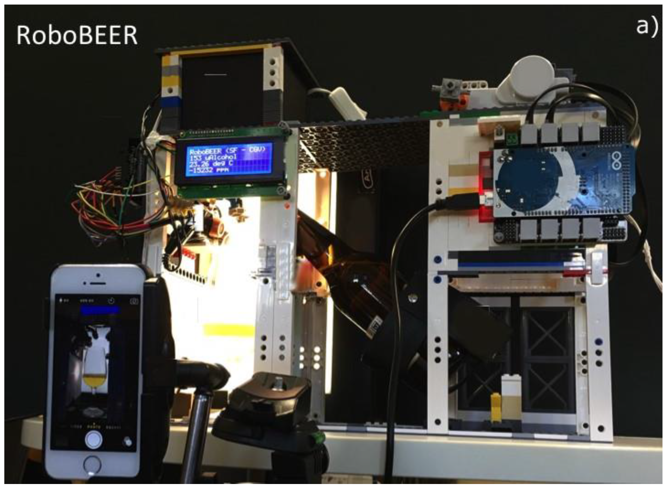
Figure 1. Equipment used to assess beers physical measurements; (a) robotic pourer, RoboBEER, which was used to assess the color and foam-related parameters and (b) a frame of a video taken to analyze the beer using computer vision algorithms.
Beverages 05 00033 g001aBeverages 05 00033 g001b
Figure 2. A two-layer feedforward model diagram showing the 15 inputs, number of neurons tested in the hidden layer, and targets/outputs used to create the model.
Beverages 05 00033 g002
Figure 3. Models showing the three stages (training, validation and testing) as well as overall model of the three best algorithms found to assess liking of beer from morpho-colorimetric parameters from beer and beer foam: (a) Levenberg Marquardt, (b) Bayesian Regularization and (c) Resilient Backpropagation, showing the correlation coefficient (R) and 95% confidence bounds. In all graphs, the x-axis represents the observed data and y-axis the predicted or estimated values. N/A = not applicable.
Beverages 05 00033 g003
Table 1. List of samples used for the study, indicating their style, country of origin and type of fermentation.
Beer StyleCountry of OriginType of Fermentation
KolschAustraliaTop
PorterPolandTop
Steam AleAustraliaTop
Sparkling AleAustraliaTop
Blonde AleBelgiumTop
Red AleUSATop
American LagerMexicoBottom
LagerThe NetherlandsBottom
PilsnerCzech RepublicBottom
American LagerUSABottom
PilsnerCzech RepublicBottom
Lambic GueuzeBelgiumSpontaneous
Lambic CassisBelgiumSpontaneous
Lambic KriekBelgiumSpontaneous
Lambic FramboiseBelgiumSpontaneous
Table 2. Algorithms used and description of the main function type and abbreviations, which were used to develop the artificial neural network models.
Main Function TypeAlgorithmAbbreviation
Backpropagation with Jacobian derivativesLevenberg MarquardtLM
Bayesian RegularizationBR
Backpropagation with gradient derivativesBroyden, Fletcher, Goldfarb, and Shanno quasi-NewtonBFGS
Conjugate gradient with Powell-Beale restartsPB
Conjugate gradient with Fletcher-Reeves updatesFR
Conjugate gradient with Polak-Ribiere updatesPR
Gradient descent backpropagationGD
Gradient descent with adaptive learning rateGDLR
Gradient descent with momentumGDM
Gradient descent with momentum and adaptive learning rateGDMLR
One step secantOSS
Resilient backpropagationRPROP
Scaled conjugate gradientSCG
Supervised weight and bias training functionsBatch training with weight and bias learning rateBLR
Cyclical order weight and biasCO
Random order weight and biasRO
Sequential order weight and biasSO
Table 3. Statistical results of the best and worse models developed using the algorithms from the three different groups. Numbers in bold represent the models with the highest correlation and determination coefficients from each group of algorithms.
AlgorithmNeuronsStageRR2bMSE
Backpropagation with Jacobian derivatives algorithm
Levenberg Marquardt7Training0.960.920.940.02
Validation0.950.901.000.06
Testing0.950.901.100.05
Overall0.950.900.980.03
Bayesian Regularization7Training0.990.980.970.01
Validation----
Testing0.970.941.10.03
Overall0.980.961.00.01
Backpropagation with gradient derivative algorithms
Gradient descent backpropagation5Training0.830.690.600.04
Validation0.670.450.390.07
Testing0.650.420.570.11
Overall0.770.590.560.06
Resilient backpropagation7Training0.950.900.900.02
Validation0.950.900.910.04
Testing0.930.860.970.04
Overall0.950.900.900.03
Supervised weight and bias algorithms
Batch training with weight and bias learning rate7Training0.800.640.590.10
Validation0.670.450.490.13
Testing0.760.580.570.11
Overall0.760.580.570.06
Random order weight and bias10Training0.890.790.820.06
Validation0.840.710.740.10
Testing0.880.771.100.06
Overall0.870.760.830.06