Article

Determination of Total Anthocyanin Concentration in Barbera Red Wines by Raman Spectroscopy and Multivariate Statistical Methods

1
Istituto Nazionale di Ricerca Metrologica (INRiM), Strada delle Cacce 91, 10135 Turin, Italy
2
Physics Department, University of Turin, Via P. Giuria 1, 10125 Turin, Italy
3
Department of Agricultural, Forest and Food Sciences, University of Turin, Corso Enotria 2/C, 12051 Alba, Italy
4
Consiglio per la Ricerca in Agricoltura e l’Analisi dell’Economia Agraria (CREA), Via Pietro Micca 35, 14100 Asti, Italy
*
Author to whom correspondence should be addressed.
Beverages 2025, 11(6), 161; https://doi.org/10.3390/beverages11060161
Submission received: 11 September 2025 / Revised: 5 November 2025 / Accepted: 12 November 2025 / Published: 17 November 2025

Abstract

The quantity of anthocyanins plays a crucial role in wine quality, since these phenolic compounds significantly influence the color, mouthfeel and organoleptic properties of red wines. It is therefore important to define accurate and precise methodologies to monitor the concentration of total anthocyanins in wine. Currently, this analysis is carried out using Ultraviolet-Visible (UV–visible) spectrophotometry. This work aims to determine an alternative methodology that is equally fast, accurate and allows in situ measurements while opening the measurement of the concentrations of other molecules of interest. The method presented consists of Raman analysis of Barbera wine samples using a portable Raman spectroscopy system. Subsequently, the collected spectra were processed using an algorithm that applies partial least squares (PLS) regression, making it possible to determine the concentration of total anthocyanins for each sample. This approach is characterized by an accuracy and precision comparable to the methodology currently in use, i.e., UV–visible spectrophotometry. It is indeed characterized by an RMSE (root mean square error) and R 2 (the coefficient of determination) on the validation set of 0.010 g/L and 0.88 and on the test data of 0.007 g/L and 0.93, respectively.

Graphical Abstract

1. Introduction

Anthocyanins are flavonoid compounds characterized by a structure consisting of two benzene rings and an oxygen-containing heterocycle. They are the glycosylated forms of anthocyanidins, pigments responsible for red coloration in acidic media, which are commonly used for anthocyanin identification and analysis. Grape anthocyanins are derived from five anthocyanidins: cyanidin, peonidin, delphinidin, petunidin, and malvidin, and contribute significantly to the sensory characteristics of red wine. They influence several sensory attributes, particularly color, which is critical as it is the first characteristic perceived by consumers and is closely linked to wine quality [1,2]. Intramolecular interactions among anthocyanins, as well as intermolecular interactions with other organic compounds, particularly phenolics, such as self-association and copigmentation, can further enhance their color expression.
During wine aging, anthocyanin concentrations decrease, which can lead to significant changes in color, mouthfeel, and overall organoleptic properties [3]. It is therefore crucial to determine accurate and precise methodologies to monitor the concentration of anthocyanins during the processes the wine undergoes before being bottled.
Traditionally, ultraviolet–visible (UV–visible) spectrophotometric methods are used to effectively quantify anthocyanins (and phenolic compounds more generally), as these compounds absorb UV and visible light at specific wavelengths [4]. The intensity of the UV–visible spectrum is attributed to the electronic transition of π-type orbitals, which depends on the number and position of the OH, O C H 3 and glycosidic groups of the different classes of polyphenols [5]. Furthermore, intermolecular interactions and the conditions of the medium (pH, metals, S O 2 ) define the UV–visible absorption of these compounds [6]. Spectrophotometric analyses of phenolic compounds are performed using consolidated protocols [7] and generally provide an estimate of the overall content of a specific subclass of phenolic compounds. The procedures commonly used to measure the amount of anthocyanins are as follows: hydrochloric acid method, bisulfite bleaching method, pH differential method, modified Somers assay and copigmentation assay [7,8]. Furthermore, by inserting a separative step by high-performance liquid chromatography (HPLC) prior to the spectrophotometric measurement, it is possible to determine the main compounds of the anthocyanin fraction in the sample [9] as expressed in the document stipulated by the International Organization of Vine and Wine (OIV) to define the official method for determining the relative composition of anthocyanins in red and rosé wines.
Because traditional methods require reagents and cannot provide real-time measurements, there is a growing need for alternative approaches to determine total anthocyanin concentrations directly and in real time. In this context, infrared and Raman spectroscopy techniques emerge as a valid and convenient methodology to measure total anthocyanin concentration in fruit, juices and wines [10,11]. In fact, they allow for rapid, non-destructive and reagent-free analysis. These methods are highly specific and sensitive and allow for on-site measurements using portable instruments [12,13].
Raman spectroscopy offers a key advantage over infrared (IR) for analyzing aqueous samples: water, which strongly absorbs in the IR range, produces a relatively weak Raman signal, particularly when high-wavelength lasers (e.g., 785 nm) are used. This makes Raman particularly suitable for the direct analysis of liquid samples, including those with a high water content. To date, phenolic analysis on grape juice and wine samples is not widely performed using Raman spectroscopy, probably because these chemical compounds do not exhibit obvious characteristics in the Raman spectra of the sample [14,15]. A work carried out on grape juice [11] led to the determination of a method using Raman spectroscopy combined with univariate linear regression, which, however, was found to be inadequate for measuring anthocyanin content. More promising, however, is the combination of Raman spectroscopy and multivariate regression, such as partial least squares (PLS) regression, which made it possible to quantitatively analyze anthocyanins in wine by means of a model characterized by an R 2 and RMSE on the validation data of 0.84 and 0.04 g/L, respectively [10]. It is important to note that the common feature of research work in this field is the application of multivariate analysis [16] and machine learning (ML) techniques. They can be combined with spectroscopy [17] to overcome the low detectability of compounds in complex matrices and are increasingly used in analytical sciences, including the analysis of wine phenolics [18,19]. Applying multivariate and machine learning techniques to spectroscopic data enables the extraction of both qualitative and quantitative information about the chemical composition of the samples [20]. Furthermore, using these methods, the model describing a training dataset can be determined to perform predictions on new, unknown datasets and greatly speed up the analysis of experimental data. Consequently, integrating traditional instrumental techniques with multivariate and ML approaches is increasingly popular for optimizing and automating sample analysis, tracking compositional changes during processes, and identifying underlying data patterns [21,22]. In this study, these techniques were used to analyze Raman spectra to identify characteristic patterns that follow the dataset and make predictions on new data.
In particular, the objective of this study is to combine Raman analysis with multivariate techniques for determining the concentration of total anthocyanins in Barbera wine samples [23]. The obtained results were then confronted with the currently most widespread technique: UV–visible spectrophotometry [24]. Raman spectroscopy may offer a promising advancement in enology by enabling faster, real-time and reagent-free predictions of anthocyanin content in wine compared to traditional methods. In addition, unlike UV–visible spectrophotometry, it allows specific compounds to be determined, such as specific anthocyanins and other molecules present in the sample (e.g., ethanol, malic acid and lactic acid) [25]. This rapid analysis could provide winemakers with critical insights into anthocyanin richness, allowing for more precise adjustments (such as preservation-stabilization techniques) during production to enhance wine quality. This new methodology was developed in the QualShelL ‘Wine Quality and Shelf-Life’ project [26], which involves the implementation of new methods for assessing the quality of grapes and monitoring winemaking processes in order to obtain high standards of wine quality.

2. Materials and Methods

2.1. Experimental Design

To evaluate the performance of Raman spectroscopy on wines with different characteristics, the Barbera wine samples (Asti, Italy) analyzed in the present study were obtained from a single batch. This was then modified to create different experimental units by introducing variations that simulate conditions present in the cellar and different levels of oxidation. Samples were analyzed over 8 months to assess the impact of aging time on wine characteristics. In total, the anthocyanin concentration of 96 samples of Barbera wine was analyzed through spectrophotometric and Raman spectroscopy.
The Raman spectra of the samples were acquired using a self-built portable instrument (Turin, Italy). The Raman spectra acquired were analyzed using multivariate analysis techniques to build a predictive model based on the concentration of total anthocyanins determined by spectrophotometry in the visible range. The final step is to determine the total anthocyanin concentration of 10 unknown Barbera wine samples by applying the newly built model.

2.2. Materials

In this experiment, the samples were obtained from 20 L of wine produced by the winemaking of grapes Vitis vinifera L. cv. Barbera, grown in Piemonte region (Italy) in the 2022 vintage. To introduce variation among the samples, the bulk wine was divided and oxygenated with increasing doses of oxygen: 7, 14, 21, and 28 mg/L, simulating conditions found in wineries and progressively higher levels of oxidation [27]. Moreover, the wine pH was either lowered to pH 3.3 using 1 mol/L HCl or raised to pH 3.6 by addition of 1 mol/L NaOH, to simulate different winemaking scenarios [28]. The eight experimental conditions, resulting from the combination of oxygenation and pH levels, were monitored at 2, 4, 6 and 8 months. For each treatment/time combination, three independent samples were prepared and analyzed, for a total of 96 experimental units (8 conditions × 4 times × 3 independent replicates). The experimental design is shown in Figure 1.

2.3. Spectrophotometric Acquisition of Barbera Wine Sample

The total anthocyanin content was measured using spectrophotometry, following a well-established method [29]. Spectrophotometric measurements were conducted using a UV–vis JASCO V-630 spectrophotometer (JASCO, Tokyo, Japan). Wine samples were diluted 50-fold in a solution of water, ethanol, and hydrochloric acid 37% in a 70:30:1 volume ratio (v/v). Samples were then transferred into an optical glass 10 mm cuvette. The absorbance was measured at 535–540 nm wavelength, and this value was used to determine anthocyanin concentration based on an external calibration curve prepared with malvidin-3-O-glucoside chloride as the standard.

2.4. Raman Spectrum Acquisition of Barbera Wine Sample

A Raman spectrum was acquired for each of the 96 experimental units, for a total of 96 spectra collected. Each sample was placed in a quartz cuvette and the Raman spectrum was acquired by directing the laser through the side wall of the cuvette, with the focal point positioned within the liquid to avoid the glass interface. The Raman spectrum of each experimental unit was obtained using a customized portable Raman device, whose specifications are described as follows:
  • Spectrometer: Exemplar Pro (B&W Tek, Plainsboro, NJ, USA) featuring a highly sensitive deep cooled (−25 °C) with a wavelength range of 190–1100 nm and a spectral resolution of 0.6 nm. Also equipped with a CCD back-illuminated (BT) detector that is highly sensitive and cooled (−25 °C);
  • Optical fiber coupled to a BAC102 Raman Trigger probe (B&W Tek, Plainsboro, NJ, USA): the latter has a working distance of 5.5 mm, while the fiber is characterized by a numerical aperture of 0.22;
  • Laser: BRM-785E (B&W Tek, Plainsboro, NJ, USA) with a wavelength of 785 nm and an output power of 300 mW;
  • Raman shift range for acquisition: [50, 3400] c m 1 ;
  • Raman spectral resolution average: 11 c m 1 ;
  • Number of scans: 3;
  • Acquisition time for each scan: 10 s.

2.5. Data Preprocessing

Before analyzing the data, it was necessary to preprocess the acquired spectra to correct and transform them for suitability in statistical analysis. The preprocessing techniques were selected empirically during the preliminary optimization phase and are described in detail below.
  • Removal of the Rayleigh peak tail (the spectral region with the lowest Raman shift) that does not contain information on the samples under examination
  • Removal of the Raman shift window from 1700 to 3400 c m 1 since it contains no relevant information on anthocyanins [30,31];
  • Noise reduction by applying the Savitzky–Golay algorithm from the SciPy library [32] (9 points window and second-order polynomial);
  • Baseline removal using asymmetric least squares (AsLS) fitting ( λ = 10 4 , p = 10 3 ). A function of the Python (version 3.12) library “pybaselines.whittaker” that provides several Whittaker-smoothing-based algorithms for fitting the baseline [33];
  • l2 normalization of the spectral intensities, in order to have spectra with the same scale (the “preprocessing.normalize” function of the scikit-learn package was used).

2.6. Application of PLS Regression

Once the data had been processed, the next step was to create the dataset. This consisted of an X-matrix containing the intensity of every Raman spectrum and a Y-vector whose elements were the total concentrations of anthocyanins (g/L) measured using the spectrophotometric method. The X matrix had dimensions M × N, in which M is equal to the total number of acquired spectra (96) and N corresponds to the number of pixels (564) associated with Raman shifts in the spectral band. Y was a column vector with dimensions M × 1 (where M is again equal to the total number of acquired spectra and 1 is the number of types of target variables). For example, the intensities of the first Raman spectrum acquired are reported in the first row of X, and the total anthocyanin concentration (determined by spectrophotometry) relative to the first sample is reported in the first element of Y.
Among the various multivariate analysis techniques, PLS (Partial Least Squares Regression) was chosen and applied, implemented using Python’s scikit-learn library [34]). PLS is particularly suited to managing datasets characterized by high collinearity between independent variables and allows for reducing dimensionality while maximizing the covariance between the X and Y matrices, thus providing greater predictive accuracy. In contrast to principal component regression (PCR), which reduces dimensionality with an unsupervised approach using principal component analysis (PCA) before applying regression, PLS integrates latent component selection directly into the supervised modeling process. For this reason, PCA analysis, which is exploratory and unsupervised in nature, was not considered, as it is primarily aimed at analyzing the internal structure of the independent variables rather than modeling the predictive relationship with the response variable [35].
Using this approach, a linear regression model can be constructed from the input data provided, after projecting them into a new space using an appropriate transformation [36]. In this new space, the data is represented by newly constructed variables called latent variables (LVs), allowing dimensionality reduction to be applied and hidden properties in the data to be highlighted.
Before determining the model (by applying PLS regression), the dataset was divided into three sets: for the training phase, for the training, validation, and testing phases, in order to perform all three phases and build a robust model. In this work, first ten samples (representing about 10% of the total dataset) were excluded from the dataset by means of a random extraction, to be employed in the test phase. Subsequently, the k-fold cross-validation (CV) technique was used to implement the training and validation phase, dividing the remaining dataset as follows: 80% for the training set and 20% for the validation set [37].

2.7. Best PLS Regression Model and Evaluation of Performance

To determine the model that best describes the data and to evaluate its accuracy, the RMSE parameter is used (in the optimal case, RMSE = 0). It is defined as the square root of the mean square error (MSE). It provides a measure of the difference between the values predicted by the model and the expected values and is defined as follows [38]:
R M S E = j = 1 n y j y j ^ 2 n
where y j are the measurements for each sample in the set, y j ^ are the expected value for each sample under examination, n is equal to the number of measurements.
The accuracy of the model can also be assessed using the coefficient of determination R 2 . This measures the proportion of variance in the dependent variable that is explained by the regression model, and in the optimal case is equal to 1.
R 2 is defined using the mean square error (MSE) and the mean total square (MST) by the following equation:
R 2 = 1 M S E M S T
The optimal model and number of latent variables were determined from the RMSE curve as a function of the number of latent variables for both the training set and the validation set. In fact, the best number of LVs corresponds to the value of the x-axis associated with the minimum RMSE on the validation set (considering a value of R 2 that is sufficiently high) [39,40].
In addition, to estimate the robustness of the model, the relative predictive determinant (RPD) was used, which follows the following criteria: RPD > 3 represents excellent prediction; 2 < RPD < 3 has limited predictive ability; RPD < 2 has no predictive ability [41]. It is given by the equation below:
R P D = σ R M S E
where σ is the standard deviation.
The selected model was then applied to the test samples, which were not used in training or validation. These will be the input for the newly constructed model, which will provide the total anthocyanin concentration as output. Finally, these measured values will be compared with the corresponding known values determined using the traditional methodology.

3. Results and Discussion

3.1. Raman Spectrum Analysis of Barbera Wine and Preprocessing

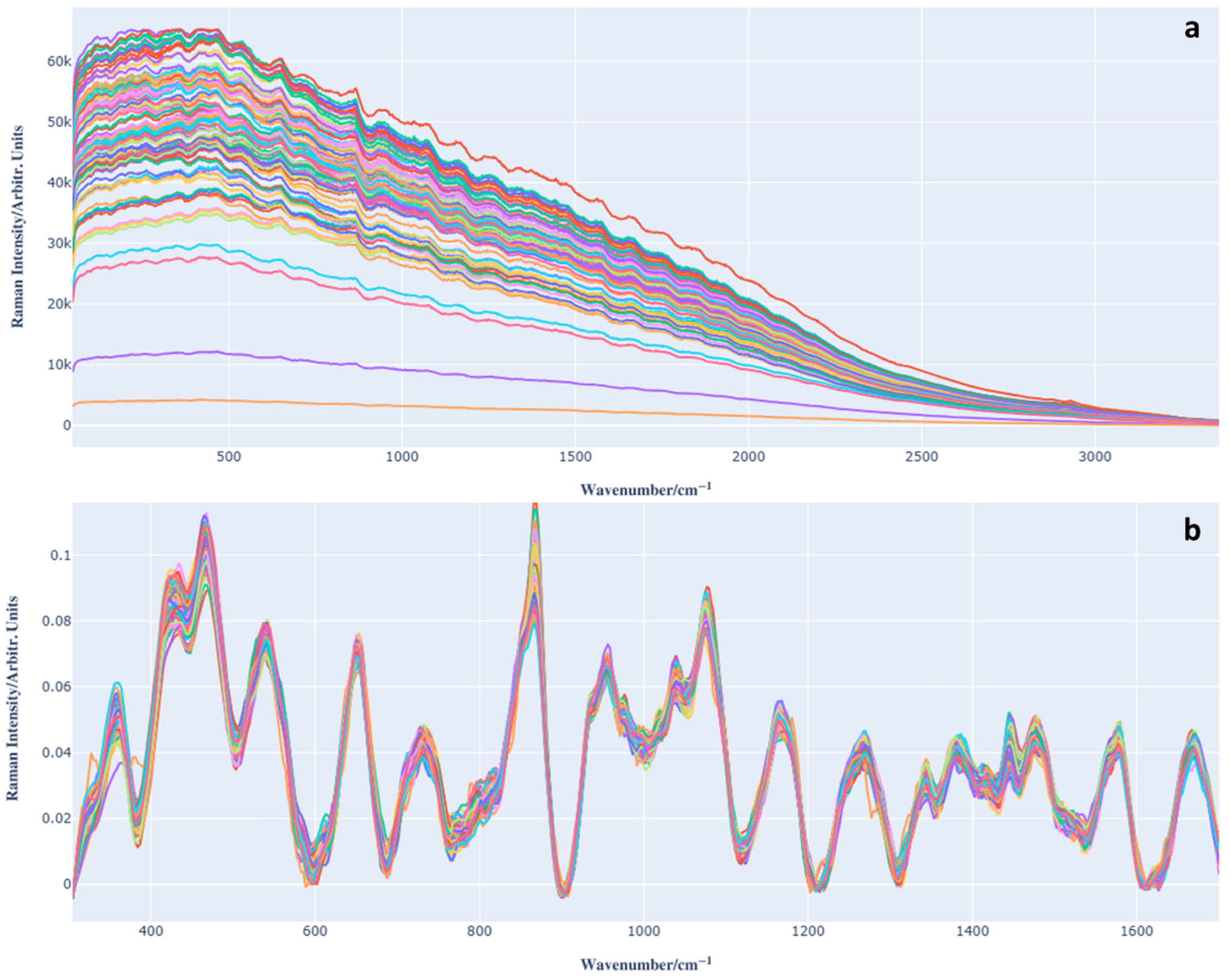
Figure 2a shows the raw acquired Raman spectra, which exhibit a baseline (caused by fluorescence) that requires correction. After acquiring the spectra and before applying PLS regression, we applied spectral preprocessing in order to minimize unwanted variability (e.g., baseline shifts, noise, and dispersion effects) and emphasize spectral features associated with the presence of anthocyanins.
This step was essential to improve both the interpretability and predictive performance of the chemometric model. The steps required for this phase are described in the subsection ‘Data preprocessing’. The spectra after preprocessing are shown in Figure 2b.
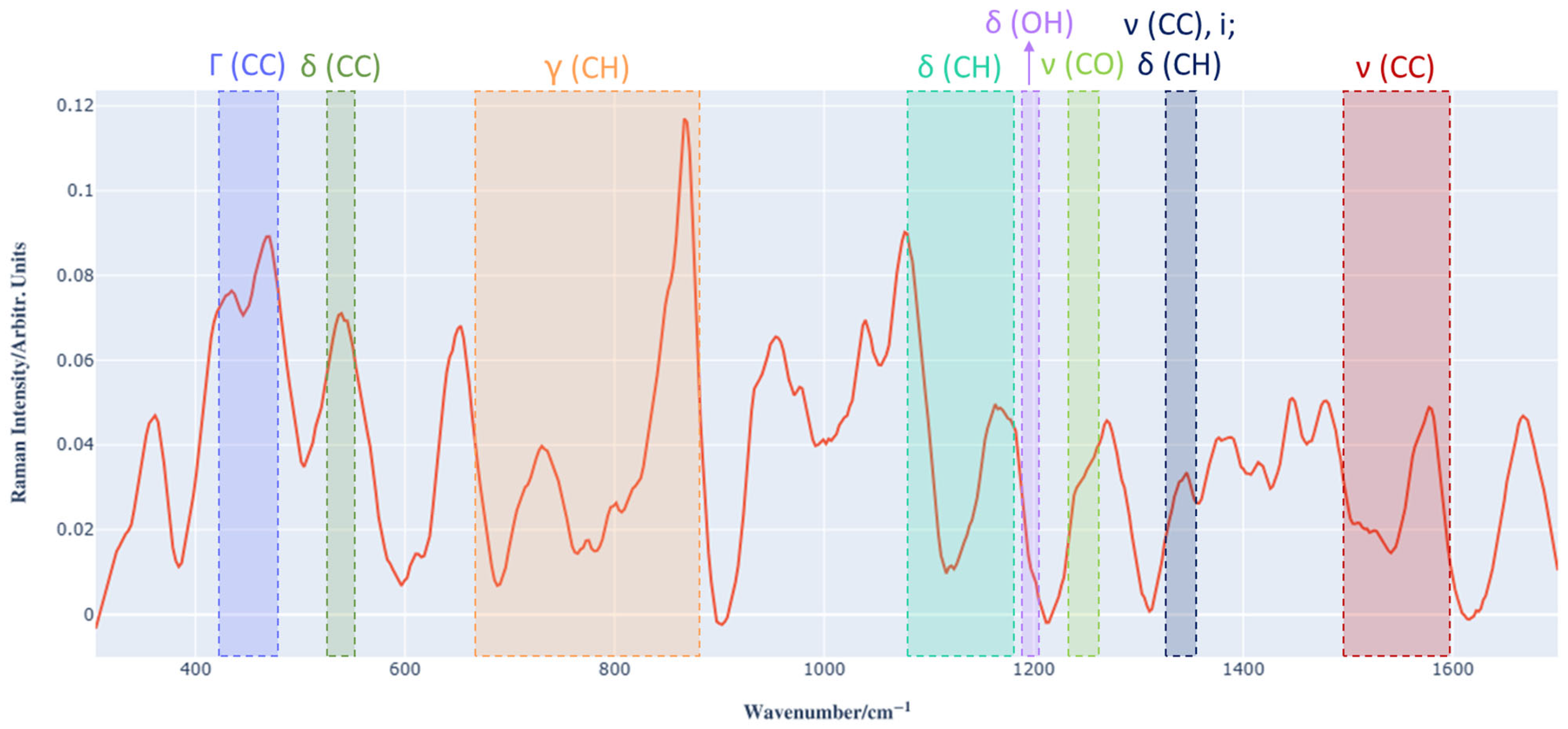
It is important to note that the Raman spectrum of the Barbera wine sample is characterized by numerous overlapping peaks due to the complex chemical composition of the sample. Figure 3 shows an example of a preprocessed Raman spectrum of Barbera wine in the dataset, in which the regions of peaks characteristic of anthocyanins are highlighted [11,31]; these are obscured or distorted by the signals of the several chemical compounds in the matrix of the wine being examined. For this reason, multivariate analysis methods are necessary to establish the correlation between the Raman spectra of wine and the concentration of total anthocyanins determined by spectrophotometry.
Table 1 shows the peak regions characteristic of anthocyanins and the main corresponding vibrational mode assigned to them [31].

3.2. PLS Regression Model

After completing the data preprocessing phase, a PLS (Partial Least Squares) regression was performed on the training set to capture the underlying structure of the data. One of the initial results of this multivariate approach is the generation of a new data representation through the use of latent variables (LVs), which allow for dimensionality reduction.
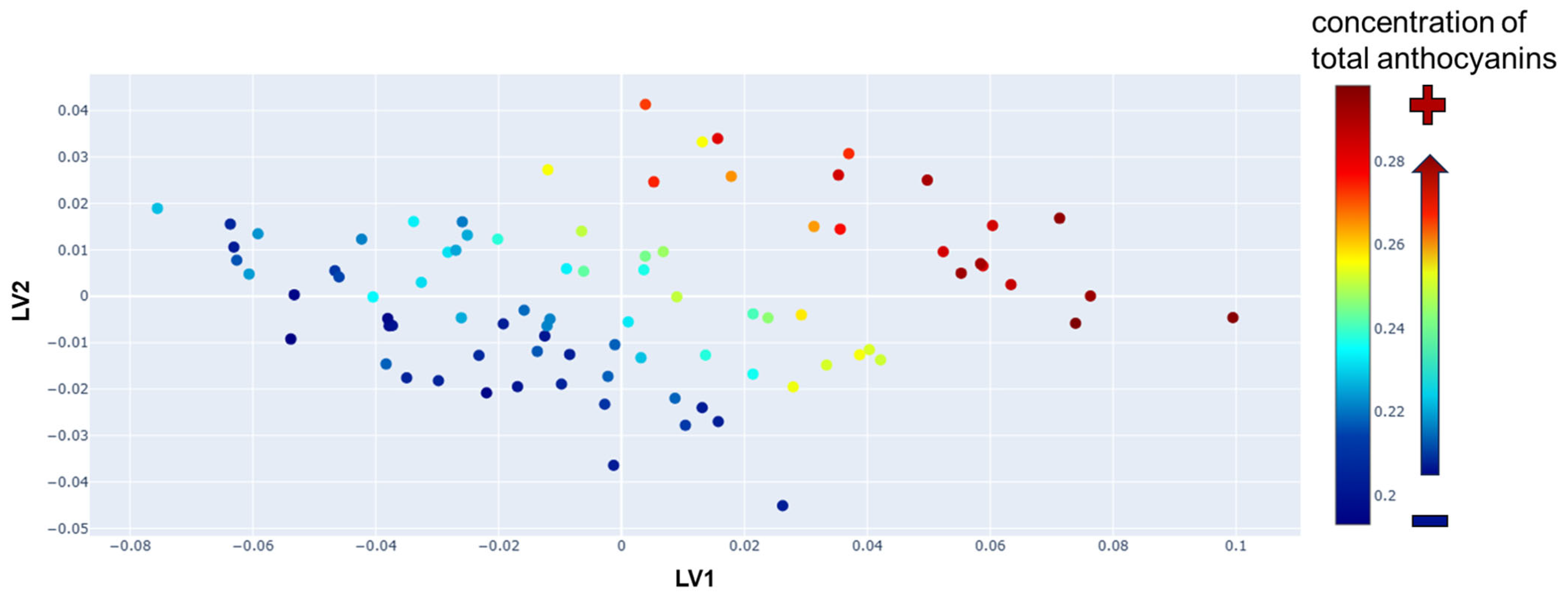
The impact of the PLS transformation is illustrated in Figure 4, where each of the 96 Raman spectra is projected onto a two-dimensional space defined by the first two latent variables, those that capture the greatest variance within the dataset. In this reduced space, each spectrum is represented as a single point characterized by its LV1 and LV2 values. Prior to this transformation, each spectrum was described by a complete row in the X matrix, consisting of 564 variables. This graphical representation reveals the intrinsic structure of the dataset, highlighting the similar and different characteristics between samples. By applying a color gradation based on the total anthocyanin concentration for each sample, a clear trend becomes evident: anthocyanin content increases progressively along the directions defined by LV1 and LV2.
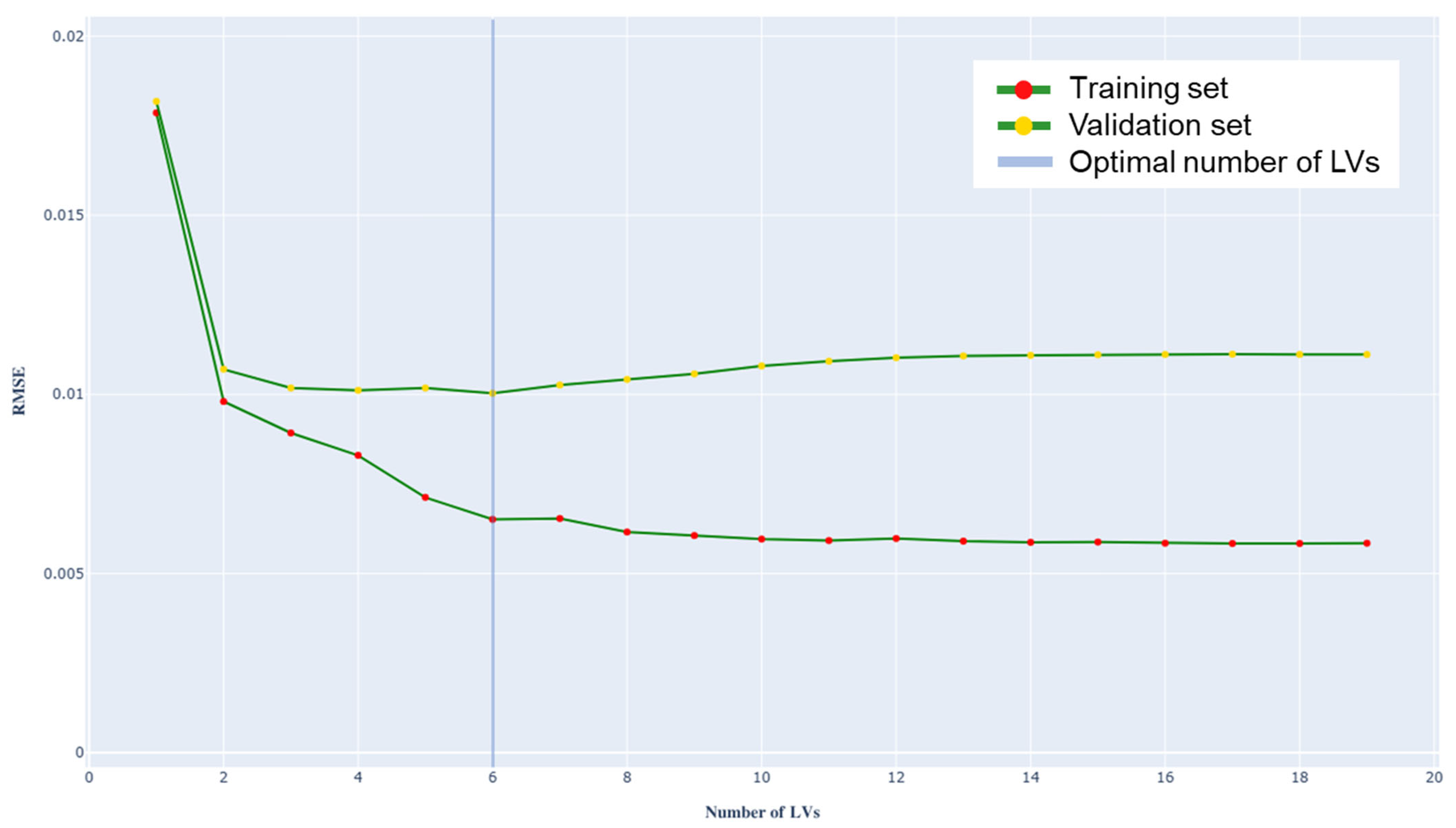
To select the most appropriate number of latent variables, the variation in RMSE was analyzed as the number of LVs increased, both for the training set and for the validation set (Figure 5). The minimum RMSE value obtained on the validation set allows the ideal number of LVs to be identified, which corresponds to the PLS model best suited to describe the data. Any further increase in LVs would lead to overfitting.
In this study, the optimal parameters obtained are:
  • RMSE = 0.010 g/L,
  • Optimal number of LVs = 6.
Figure 5 presents the plot of RMSE as a function of the number of LVs.
It was also possible to assess goodness and robustness of the model using the R 2 and RPD, respectively, which on the validation set are 0.88 and 2.94.
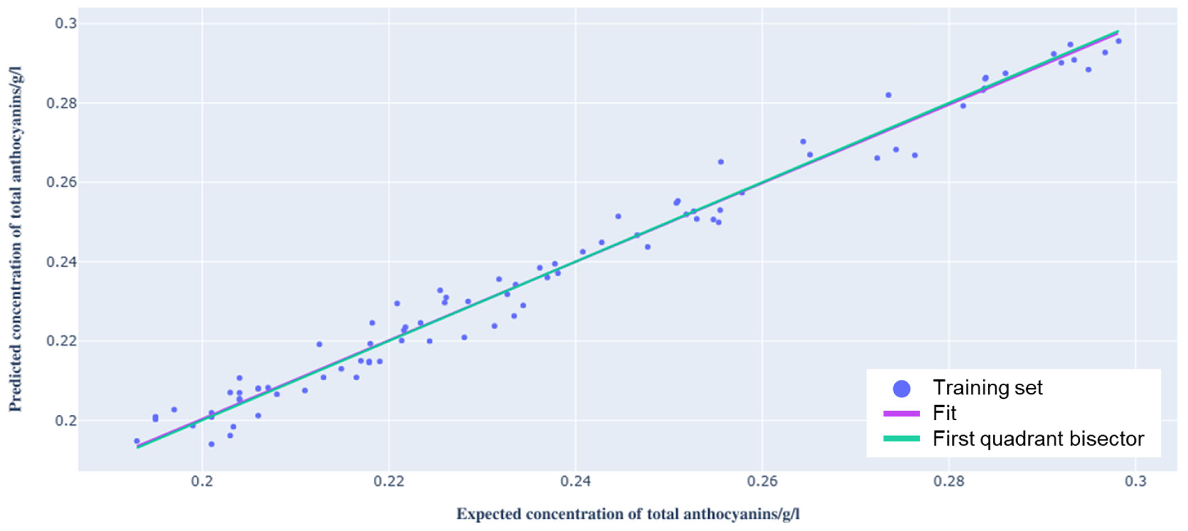
In order to assess the validity of the model’s performance, a graph of the total anthocyanin concentration measured by spectrophotometry can be plotted as a function of that predicted by the model (Figure 6). The training set spectra are represented by blue points, and their linear fit is defined by the purple curve. Finally, the green curve represents the expected theoretical trend, i.e., the condition in which the total anthocyanin concentrations obtained with the two methods coincide. This is effectively the bisector of the first quadrant. The linear fit of the training set data points was calculated by applying the ordinary least squares (OLS) regression on these data.
The fit parameters (the slope m and the intercept q), Z-test, and p-value are shown in Table 2.
It is also possible to analyze the loadings as a function of RS in order to identify the most significant spectral regions for model construction. The most relevant Raman shifts correspond to the values with the highest absolute ordinates. RS regions most influential in determining the model for the first latent variables (LVs) correspond to the skeleton out-of-plane bending (Γ) of the CC bond and the out-of-plane bending (γ) of the CH bond. Figure S1 (Supporting Information) shows the graph of the loadings referring to the first latent variable. For the second LV, the most important RS windows are: out-of-plane bending (γ) of the CH bond, in-plane bending (δ) of the CC and CH bonds, and stretching (ν) of the CC bond (as can be seen in Figure S2 of the Supporting Information).
The sum of the variance explained by the six latent variables used by the model allows quantification of the proportion of information preserved after data transformation. In the new representation, the retained variance is 54% for X and 98% for Y. Figure S3 (Supporting Information) shows the graph of the variance explained by the X matrix (Raman spectra) and the explained and cumulative variance by the Y vector (total anthocyanin concentration) in the latent variables considered.

3.3. Testing New Data

We applied the model to ten Barbera wine samples, randomly selected from the dataset, to estimate the total anthocyanin concentration. Using the spectra from the test set instead of those from the training set, the results shown in Figure 7 were obtained. The confidence interval, calculated with a significance level of 5%, is highlighted in orange.
To determine the accuracy of the model’s prediction on the test set, the RMSE parameter was used (defined as discussed in the subsection “Best PLS regression model and performance evaluation”), where y j are the values measured by Raman spectroscopy, y j ^ are the expected values obtained by spectrophotometry, and n is equal to the number of samples considered, in this case equal to 10. It is obtained: R M S E = 0.007 g/L.
In the optimal scenario, this parameter would be zero, indicating that the model can accurately predict the total anthocyanin concentration in unknown samples.

3.4. Comparison of Spectrophotometry and Raman Spectroscopy

Finally, a comparison between the total anthocyanin concentration predicted by the model and that provided spectrophotometrically for the ten unknown Barbera wine samples is reported. The associated with anthocyanin concentration is provided by the model, while the uncertainty was calculated as the standard deviation of the linear regression residuals ( σ y ):
σ y =   1 N 2   i = 1 N y i q + m · x i 2 =   0.008   g / L
where N is equal to the number of samples in the test set, y i and x i are, respectively, the total anthocyanin concentration predicted by the model and measured spectrophotometrically, and q and m are, respectively, the intercept and the slope of the fit.
The total anthocyanin concentration values measured using the two techniques, the Z-test and the p-value for the set test, are shown in Table 3. The uncertainties associated with the expected values provided by visible spectrophotometry are the standard deviations of three repetitions for each sample.
Analysis of the values shown in Table 3 indicates that the concentrations determined by Raman spectroscopy were consistent with those obtained by spectrophotometry. Indeed, performing a Z-test on the results of the unknown samples yields a p-value greater than 0.05 for all samples. This implies that the difference between the observed measure and the expected value is not statistically significant, i.e., that the observations are consistent with expectations. Therefore, the predictions on the test set and the corresponding expected values are comparable with each other, and the results obtained from the model are accurate and precise. In fact, on the test set, the RMSE is 0.007 g/L, the RPD is 3.86 and R 2   =   0.93 .
Finally, a summary of the model performance evaluation parameters for training, validation and test set is given in Table 4.

4. Conclusions

This study employed an integrated Raman spectroscopy-multivariate modeling method to quantify the total anthocyanin concentration in Barbera wine samples. This new methodology is a viable alternative to the currently used technique. It enables in situ, rapid, and non-destructive measurements using a portable Raman device. It does not require the use of reagents and allows real-time monitoring of the concentration of total anthocyanins in Barbera wine samples. Furthermore, unlike UV–vis spectrophotometry, it potentially allows the simultaneous determination of specific compounds, such as specific anthocyanins and other molecules present in the wine sample (e.g., ethanol, malic acid and lactic acid).
To analyze the chemical compound in question, two simple steps are followed: the Raman spectrum of the wine sample is acquired and the multivariate regression model is applied. Finally, the model will provide the total concentration of anthocyanins characteristic of the sample (in g/L) using a method characterized by high specificity and sensitivity.
The PLS regression model constructed demonstrates good accuracy, in fact the RMSE on the CV set and test set are 0.01 and 0.007 g/L, respectively. It is characterized by R 2 on the validation set and test set equal to 0.88 and 0.93, respectively (for concentrations in the typical range of Barbera wine). Furthermore, the measurements obtained on the test set are characterized by a percentage relative uncertainty of 3.5%. In conclusion, the data collected confirm that the Raman-PLS approach is a valid technique for quantifying the total concentration of anthocyanins, offering levels of accuracy and precision comparable to those obtained using visible spectrophotometry. Raman spectroscopy could significantly benefit enology by offering a quicker, real-time method for predicting the content of anthocyanins and potentially other chemical compounds present in wine, providing a faster alternative to traditional methods. By delivering real-time data on phenolic composition, this technique enables winemakers to make precise, data-driven adjustments throughout the wine production process, helping them to optimize wine quality.
However, it is important to acknowledge some limitations of this study. The investigation was conducted on a limited number of samples belonging to a single variety (Barbera wine), which may reduce the generalizability of the model to other types of wine. Furthermore, Raman spectra can be affected by fluorescence background and instrumental noise, factors that can reduce sensitivity to low concentrations of the chemical compound under examination.
Future studies should therefore include a larger number of samples from different varieties, vintages, and storage conditions, as well as explore advanced preprocessing and correction techniques to minimize spectral interference. A further development could involve extending the approach to the specific determination of individual anthocyanins or other key phenolic compounds, in order to enhance the analytical and applicative value of the proposed methodology.

Supplementary Materials

The following supporting information can be downloaded at: https://www.mdpi.com/article/10.3390/beverages11060161/s1, Figure S1: First LV as a function of RS; Figure S2: Second LV as a function of RS; Figure S3: Variance explained X (intensity of Raman spectra) and Y (concentration of total anthocyanins).

Author Contributions

Conceptualization, A.S., A.B. and A.M.R.; methodology, A.L.G., A.S., S.G. and L.F.; software, A.L.G.; validation, A.L.G., S.G. and L.F.; formal analysis, A.L.G., A.S., S.G. and L.F.; investigation, A.L.G., A.S., S.G. and L.F.; resources, A.B. and A.M.R.; data curation, A.L.G.; writing—original draft preparation, A.L.G.; writing—review and editing, A.L.G., A.S., A.M.G., S.G., A.B., L.P., L.F., S.R.B., S.M. (Stefano Messina)., M.L., S.M. (Silvia Motta), M.G., E.V. and A.M.R.; visualization, A.L.G.; supervision, A.S., A.M.G., E.V. and A.M.R.; project administration, A.B.; funding acquisition, A.B. and A.M.R. All authors have read and agreed to the published version of the manuscript.

Funding

This work was funded through the PSR QualShelL by Regione Piemonte—Programma di Sviluppo Rurale (FEASR) operazione 16.1.1 (CUP code: J66B20006290002).

Institutional Review Board Statement

Not applicable.

Informed Consent Statement

Not applicable.

Data Availability Statement

Dataset available on request from the authors.

Acknowledgments

During the preparation of this manuscript, the authors used a portable Raman apparatus and a UV-visible spectrophotometer for Raman and spectrophotometric analysis, respectively. Raman spectrum analysis was performed using Python (version 3.12). The authors reviewed and edited the result and take full responsibility for the content of this publication.

Conflicts of Interest

The authors declare no conflicts of interest.

Abbreviations

AsLSAsymmetric least squares
BTBack-thinned
CCDCharge-coupled device
CVCross validation
HPLCHigh-performance liquid chromatography
LVLatent variable
MLMachine learning
MSEMean square error
MSTMean total sum
OIVInternational organization of vine and wine
PCRPrincipal component regression
PLSPartial least square
RMSERoot mean square error
RPDRelative predictive determinant
UVUltraviolet
VISVisible

References

  1. Chen, H.; Wang, M.; Zhang, L.; Ren, F.; Li, Y.; Chen, Y.; Liu, Y.; Zhang, Z.; Zeng, Q. Anthocyanin Profiles and Color Parameters of Fourteen Grapes and Wines from the Eastern Foot of Helan Mountain in Ningxia. Food Chem. X 2024, 24, 102034. [Google Scholar] [CrossRef] [PubMed]
  2. Mazza, G.; Fukumoto, L.; Delaquis, P.; Girard, B.; Ewert, B. Anthocyanins, Phenolics, and Color of Cabernet Franc, Merlot, and Pinot Noir Wines from British Columbia. J. Agric. Food Chem. 1999, 47, 4009–4017. [Google Scholar] [CrossRef]
  3. Ofoedu, C.E.; Ofoedu, E.O.; Chacha, J.S.; Owuamanam, C.I.; Efekalam, I.S.; Awuchi, C.G. Comparative Evaluation of Physicochemical, Antioxidant, and Sensory Properties of Red Wine as Markers of Its Quality and Authenticity. Int. J. Food Sci. 2022, 2022, 8368992. [Google Scholar] [CrossRef]
  4. Lorrain, B.; Ky, I.; Pechamat, L.; Teissedre, P.-L. Evolution of Analysis of Polyhenols from Grapes, Wines, and Extracts. Molecules 2013, 18, 1076–1100. [Google Scholar] [CrossRef]
  5. Sanna, R.; Piras, C.; Marincola, F.C.; Lecca, V.; Maurichi, S.; Scano, P. Multivariate Statistical Analysis of the UV-Vis Profiles of Wine Polyphenolic Extracts during Vinification. J. Agric. Sci. 2014, 6, 152. [Google Scholar] [CrossRef]
  6. Gierschner, J.; Duroux, J.-L.; Trouillas, P. UV/Visible Spectra of Natural Polyphenols: A Time-Dependent Density Functional Theory Study. Food Chem. 2012, 131, 79–89. [Google Scholar]
  7. Aleixandre-Tudo, J.L.; Buica, A.; Nieuwoudt, H.; Aleixandre, J.L.; du Toit, W. Spectrophotometric Analysis of Phenolic Compounds in Grapes and Wines. J. Agric. Food Chem. 2017, 65, 4009–4026. [Google Scholar] [CrossRef] [PubMed]
  8. Harbertson, J.F.; Spayd, S. Measuring Phenolics in the Winery. Am. J. Enol. Vitic. 2006, 57, 280–288. [Google Scholar] [CrossRef]
  9. de Andrade, R.H.S.; do Nascimento, L.S.; Pereira, G.E.; Hallwass, F.; Paim, A.P.S. Anthocyanic Composition of Brazilian Red Wines and Use of HPLC-UV–Vis Associated to Chemometrics to Distinguish Wines from Different Regions. Microchem. J. 2013, 110, 256–262. [Google Scholar] [CrossRef]
  10. Gallego, Á.L.; Guesalaga, A.R.; Bordeu, E.; Gonzalez, Á.S. Rapid Measurement of Phenolics Compounds in Red Wine Using Raman Spectroscopy. IEEE Trans. Instrum. Meas. 2011, 60, 507–512. [Google Scholar] [CrossRef]
  11. Gao, Z.; Yang, G.; Zhao, X.; Jiao, L.; Wen, X.; Liu, Y.; Xia, X.; Zhao, C.; Dong, D. Rapid Measurement of Anthocyanin Content in Grape and Grape Juice: Raman Spectroscopy Provides Non-Destructive, Rapid Methods. Comput. Electron. Agric. 2024, 222, 109048. [Google Scholar] [CrossRef]
  12. Duan, C.; Xiao, X.; Yu, Y.; Xu, M.; Zhang, Y.; Liu, X.; Dai, H.; Pi, F.; Wang, J. In Situ Raman Characterization of the Stability of Blueberry Anthocyanins in Aqueous Solutions under Perturbations in Temperature, UV, pH. Food Chem. 2024, 431, 137155. [Google Scholar] [CrossRef]
  13. Liu, H.; Cao, L.; Sui, J.; Lin, H.; Wang, X.; Wang, K. Unveiling Anthocyanins Structural Basis with Multiplexed Colorimetric and SERS Responses for Smart Monitoring of Seafood Freshness. Food Chem. 2025, 488, 144841. [Google Scholar] [CrossRef]
  14. Fuller, H.; Beaver, C.; Harbertson, J. Alcoholic Fermentation Monitoring and pH Prediction in Red and White Wine by Combining Spontaneous Raman Spectroscopy and Machine Learning Algorithms. Beverages 2021, 7, 78. [Google Scholar] [CrossRef]
  15. Lu, B.; Tian, F.; Chen, C.; Wu, W.; Tian, X.; Chen, C.; Lv, X. Identification of Chinese Red Wine Origins Based on Raman Spectroscopy and Deep Learning. Spectrochim. Acta A Mol. Biomol. Spectrosc. 2023, 291, 122355. [Google Scholar] [CrossRef] [PubMed]
  16. Ezenarro, J.; Schorn-García, D. How Are Chemometric Models Validated? A Systematic Review of Linear Regression Models for NIRS Data in Food Analysis. J. Chemom. 2025, 39, e70036. [Google Scholar] [CrossRef]
  17. Htet, T.T.M.; Cruz, J.; Khongkaew, P.; Suwanvecho, C.; Suntornsuk, L.; Nuchtavorn, N.; Limwikrant, W.; Phechkrajang, C. PLS-Regression-Model-Assisted Raman Spectroscopy for Vegetable Oil Classification and Non-Destructive Analysis of Alpha-Tocopherol Contents of Vegetable Oils. J. Food Compos. Anal. 2021, 103, 104119. [Google Scholar] [CrossRef]
  18. Xiao, L.; Liu, J.; Hua, M.Z.; Lu, X. Rapid Determination of Total Phenolic Content and Antioxidant Capacity of Maple Syrup Using Raman Spectroscopy and Deep Learning. Food Chem. 2025, 463, 141289. [Google Scholar] [CrossRef]
  19. dos Santos, I.; Bosman, G.; Aleixandre-Tudo, J.L.; du Toit, W. Direct Quantification of Red Wine Phenolics Using Fluorescence Spectroscopy with Chemometrics. Talanta 2022, 236, 122857. [Google Scholar] [CrossRef]
  20. Wang, T.; Xie, C.; You, Q.; Tian, X.; Xu, X. Qualitative and Quantitative Analysis of Four Benzimidazole Residues in Food by Surface-Enhanced Raman Spectroscopy Combined with Chemometrics. Food Chem. 2023, 424, 136479. [Google Scholar] [CrossRef]
  21. Wen, Y.; Li, Z.; Ning, Y.; Yan, Y.; Li, Z.; Wang, N.; Wang, H. Portable Raman Spectroscopy Coupled with PLSR Analysis for Monitoring and Predicting of the Quality of Fresh-Cut Chinese Yam at Different Storage Temperatures. Spectrochim. Acta A Mol. Biomol. Spectrosc. 2024, 310, 123956. [Google Scholar] [CrossRef] [PubMed]
  22. Castro, R.C.; Ribeiro, D.S.M.; Santos, J.L.M.; Páscoa, R.N.M.J. The Use of In-Situ Raman Spectroscopy to Monitor at Real Time the Quality of Different Types of Edible Oils under Frying Conditions. Food Control 2022, 136, 108879. [Google Scholar] [CrossRef]
  23. Ewing-Mulligan, M.; McCarthy, E. Italian Wine for Dummies; John Wiley & Sons: Hoboken, NJ, USA, 2011. [Google Scholar]
  24. Torchio, F.; Cagnasso, E.; Gerbi, V.; Rolle, L. Mechanical Properties, Phenolic Composition and Extractability Indices of Barbera Grapes of Different Soluble Solids Contents from Several Growing Areas. Anal. Chim. Acta 2010, 660, 183–189. [Google Scholar] [CrossRef]
  25. Gilioli, A.L.; Sacco, A.; Giovannozzi, A.M.; Giacosa, S.; Bosso, A.; Panero, L.; Barera, S.R.; Messina, S.; Lagori, M.; Motta, S.; et al. Raman Spectroscopy as a Rapid Tool for Monitoring Lactic Acid Concentration during Wine Malolactic Fermentation Directly in the Winery. Talanta Open 2025, 12, 100494. [Google Scholar] [CrossRef]
  26. OIV HPLC-Determination of Nine Major Anthocyanins in Red and Rosé Wine. Available online: https://www.oiv.int/standards/annex-a-methods-of-analysis-of-wines-and-musts/section-3-chemical-analysis/section-3-1-organic-compounds/section-3-1-5-other-organic-compounds/hplc-determination-of-nine-major-anthocyanins-in-red-and-rose-wines-%28type-ii%29 (accessed on 10 November 2025).
  27. Petrozziello, M.; Torchio, F.; Piano, F.; Giacosa, S.; Ugliano, M.; Bosso, A.; Rolle, L. Impact of Increasing Levels of Oxygen Consumption on the Evolution of Color, Phenolic, and Volatile Compounds of Nebbiolo Wines. Front. Chem. 2018, 6, 137. [Google Scholar] [CrossRef]
  28. Comuzzo, P.; Battistutta, F. Chapter 2—Acidification and pH Control in Red Wines. In Red Wine Technology; Morata, A., Ed.; Academic Press: Cambridge, MA, USA, 2019; pp. 17–34. ISBN 978-0-12-814399-5. [Google Scholar]
  29. Di Stefano, R.; Genfilini, N. Per Lo Studio Dei Polifenoli. L’enotecnico 1989, 5, 83–90. [Google Scholar]
  30. Bruni, S.; Longoni, M.; Minzoni, C.; Basili, M.; Zocca, I.; Pieraccini, S.; Sironi, M. Resonance Raman and Visible Micro-Spectroscopy for the In-Vivo and In-Vitro Characterization of Anthocyanin-Based Pigments in Blue and Violet Flowers: A Comparison with HPLC-ESI- MS Analysis of the Extracts. Molecules 2023, 28, 1709. [Google Scholar] [CrossRef]
  31. Zaffino, C.; Russo, B.; Bruni, S. Surface-Enhanced Raman Scattering (SERS) Study of Anthocyanidins. Spectrochim. Acta A Mol. Biomol. Spectrosc. 2015, 149, 41–47. [Google Scholar] [CrossRef] [PubMed]
  32. Virtanen, P.; Gommers, R.; Oliphant, T.E.; Haberland, M.; Reddy, T.; Cournapeau, D.; Burovski, E.; Peterson, P.; Weckesser, W.; Bright, J.; et al. SciPy 1.0: Fundamental Algorithms for Scientific Computing in Python. Nat. Methods 2020, 17, 261–272. [Google Scholar] [CrossRef] [PubMed]
  33. Peng, J.; Peng, S.; Jiang, A.; Wei, J.; Li, C.; Tan, J. Asymmetric Least Squares for Multiple Spectra Baseline Correction. Anal. Chim. Acta 2010, 683, 63–68. [Google Scholar] [CrossRef]
  34. Pedregosa, F.; Varoquaux, G.; Gramfort, A.; Michel, V.; Thirion, B.; Grisel, O.; Blondel, M.; Prettenhofer, P.; Weiss, R.; Dubourg, V.; et al. Scikit-Learn: Machine Learning in Python. J. Mach. Learn. Res. 2011, 12, 2825–2830. [Google Scholar]
  35. Dumancas, G.G.; Ramasahayam, S.; Bello, G.; Hughes, J.; Kramer, R. Chemometric Regression Techniques as Emerging, Powerful Tools in Genetic Association Studies. TrAC Trends Anal. Chem. 2015, 74, 79–88. [Google Scholar] [CrossRef]
  36. Wold, S.; Sjöström, M.; Eriksson, L. PLS-Regression: A Basic Tool of Chemometrics. Chemom. Intell. Lab. Syst. 2001, 58, 109–130. [Google Scholar] [CrossRef]
  37. Nti, I.K.; Nyarko-Boateng, O.; Aning, J. Performance of Machine Learning Algorithms with Different K Values in K-Fold Cross-Validation. Int. J. Inf. Technol. Comput. Sci. 2021, 13, 61–71. [Google Scholar]
  38. Chicco, D.; Warrens, M.J.; Jurman, G. The Coefficient of Determination R-Squared Is More Informative than SMAPE, MAE, MAPE, MSE and RMSE in Regression Analysis Evaluation. PeerJ Comput. Sci. 2021, 7, e623. [Google Scholar] [CrossRef]
  39. Moncunill, X.C. Laser-Induced Breakdown Spectroscopy (LIBS): A Potential Quality Tool for Infant Formula Manufacture. Ph.D. Thesis, Technological University Dublin, Dublin, Ireland, 2019. [Google Scholar]
  40. Matese, A.; Di Gennaro, S.F.; Orlandi, G.; Gatti, M.; Poni, S. Assessing Grapevine Biophysical Parameters From Unmanned Aerial Vehicles Hyperspectral Imagery. Front. Plant Sci. 2022, 13, 898722. [Google Scholar] [CrossRef] [PubMed]
  41. Liu, J.; Xie, J.; Han, J.; Wang, H.; Sun, J.; Li, R.; Li, S. Visible and Near-Infrared Spectroscopy with Chemometrics Are Able to Predict Soil Physical and Chemical Properties. J. Soils Sediments 2020, 20, 2749–2760. [Google Scholar] [CrossRef]
Figure 1. Experimental design.
Beverages 11 00161 g001
Figure 2. (a) Raman spectra of Barbera wine samples (different colours for each acquisition). (b) Preprocessed Raman spectra (different colours for each acquisition).
Beverages 11 00161 g002
Figure 3. Example of a Raman spectrum of Barbera wine (red signal) highlighting the regions of peaks characteristic of anthocyanins. ν (stretching), δ (in-plane bending), γ (out-of-plane bending), Γ (skeleton out-of-plane bending) and i (inter-ring stretching).
Beverages 11 00161 g003
Figure 4. Representation of the first two latent variables (LVs) as calculated by the Partial Least Squares (PLS) model. Each Raman spectrum is represented by a single point, colored based on the total concentration of anthocyanins in the wine sample (in g/L).
Beverages 11 00161 g004
Figure 5. Root mean square error (RMSE) graph as a function of the number of latent variables (for the training and validation set).
Beverages 11 00161 g005
Figure 6. Graph showing the total anthocyanin concentration predicted by the model as a function of that provided by spectrophotometric analysis (training set).
Beverages 11 00161 g006
Figure 7. Total anthocyanin concentration provided by the model based on Raman spectra as a function of that determined by spectrophotometry for the test set.
Beverages 11 00161 g007
Table 1. Assigned vibrational mode and Raman shift window containing the corresponding peak(s).
Assigned Vibrational Mode Peak   Regions   Characteristic   [ c m 1 ]
Γ (CC)424–483
δ (CC)535–545
γ (CH)670–875
δ (CH)1081–1172
δ (OH)1190–1197
ν (CO)1243–1254
ν (CC), i; δ (CH)1325–1346
ν (CC)1496–1645
ν (stretching), δ (in-plane bending), γ (out-of-plane bending), Γ (skeleton out-of-plane bending) and i (inter-ring stretching).
Table 2. Fit parameters and statistical test.
Fit ParametersMeasurementsExpected ValuesZ Testp-Value
m0.99 ± 0.021−0.660.51
q0.002 ± 0.004 g/L0 g/L0.650.52
Table 3. Total anthocyanin concentration determined using the two methods for the ten samples in the test set.
SampleTotal Anthocyanin Concentration by Spectrophotometry (g/L)Total Anthocyanin Concentration by Raman Spectroscopy (g/L)Z-Testp-Value
10.238 ± 0.0010.233 ± 0.008−0.640.52218
20.267 ± 0.0100.256 ± 0.008−1.410.15854
30.195 ± 0.0010.192 ± 0.008−0.400.68916
40.268 ± 0.0020.270 ± 0.0080.260.79486
50.246 ± 0.0040.232 ± 0.008−1.800.07186
60.273 ± 0.0020.269 ± 0.008−0.440.65994
70.206 ± 0.0010.203 ± 0.008−0.420.67448
80.224 ± 0.0010.216 ± 0.008−1.080.28014
90.207 ± 0.0020.205 ± 0.008−0.170.86502
100.230 ± 0.0020.224 ± 0.008−0.770.4413
Table 4. Summary of model performance evaluation parameters.
Set\ParametersRMSE (g/L)RPD R 2
Training0.0047.040.98
Validation0.0102.940.88
Test0.0073.860.93
Disclaimer/Publisher’s Note: The statements, opinions and data contained in all publications are solely those of the individual author(s) and contributor(s) and not of MDPI and/or the editor(s). MDPI and/or the editor(s) disclaim responsibility for any injury to people or property resulting from any ideas, methods, instructions or products referred to in the content.