Article

Improving Operational Short- to Medium-Range (SR2MR) Streamflow Forecasts in the Upper Zambezi Basin and Its Sub-Basins Using Variational Ensemble Forecasting

by
Rodrigo Valdés-Pineda
1,*,
Juan B. Valdés
1,
Sungwook Wi
2,
Aleix Serrat-Capdevila
3 and
Tirthankar Roy
4
1
Department of Hydrology and Atmospheric Sciences, University of Arizona, J W Harshbarger Bldg., 1133 James E. Rogers Way #122, Tucson, AZ 85721, USA
2
Department of Civil and Environmental Engineering, University of Massachusetts, Amherst, MA 01003, USA
3
Global Water Practice, The World Bank, Washington, DC 20433, USA
4
Department of Civil and Environmental Engineering, College of Engineering, University of Nebraska, 900 N. 16th St., Lincoln, NE 68588, USA
*
Author to whom correspondence should be addressed.
Hydrology 2021, 8(4), 188; https://doi.org/10.3390/hydrology8040188
Submission received: 2 November 2021 / Revised: 6 December 2021 / Accepted: 15 December 2021 / Published: 20 December 2021

Abstract

:
The combination of Hydrological Models and high-resolution Satellite Precipitation Products (SPPs) or regional Climatological Models (RCMs), has provided the means to establish baselines for the quantification, propagation, and reduction in hydrological uncertainty when generating streamflow forecasts. This study aimed to improve operational real-time streamflow forecasts for the Upper Zambezi River Basin (UZRB), in Africa, utilizing the novel Variational Ensemble Forecasting (VEF) approach. In this regard, we describe and discuss the main steps required to implement, calibrate, and validate an operational hydrologic forecasting system (HFS) using VEF and Hydrologic Processing Strategies (HPS). The operational HFS was constructed to monitor daily streamflow and forecast them up to eight days in the future. The forecasting process called short- to medium-range (SR2MR) streamflow forecasting was implemented using real-time rainfall data from three Satellite Precipitation Products or SPPs (The real-time TRMM Multisatellite Precipitation Analysis TMPA-RT, the NOAA CPC Morphing Technique CMORPH, and the Precipitation Estimation from Remotely Sensed data using Artificial Neural Networks, PERSIANN) and rainfall forecasts from the Global Forecasting System (GFS). The hydrologic preprocessing (HPR) strategy considered using all raw and bias corrected rainfall estimates to calibrate three distributed hydrological models (HYMOD_DS, HBV_DS, and VIC 4.2.b). The hydrologic processing (HP) strategy considered using all optimal parameter sets estimated during the calibration process to increase the number of ensembles available for operational forecasting. Finally, inference-based approaches were evaluated during the application of a hydrological postprocessing (HPP) strategy. The final evaluation and reduction in uncertainty from multiple sources, i.e., multiple precipitation products, hydrologic models, and optimal parameter sets, was significantly achieved through a fully operational implementation of VEF combined with several HPS. Finally, the main challenges and opportunities associated with operational SR2MR streamflow forecasting using VEF are evaluated and discussed.

1. Introduction

1.1. Decisions and Limitations of Hydrologic Forecasting

At any spatiotemporal scale, critical decisions about the design, functionality, and operability of a Hydrologic Forecasting System (HFS) need to be made to reduce the total hydrologic uncertainty (THU) propagated from different components of a hydrologic modelling paradigm (HMP). In fact, reducing the total hydrological uncertainty is key to developing reliable Integrated Water Resources Management (IWRM) strategies across spatial and temporal scales. For river basins across the world, the allocation of water resources largely relies on accurate streamflow forecasts. In Africa, for instance, the waters of the Upper Zambezi River Basin (UZRB) are shared by eight countries: Angola, Namibia, Zambia, Botswana, Malawi, Tanzania, Zimbabwe, and Mozambique. However, the administrative complexities created by the transnational nature of the Zambezi Basin (Figure 1) result in inconsistencies in the operation and maintenance of the rain gauges and stream gauges (see Table 1), and consequently a lack of reliable hydrologic data for the implementation of an HFS. For example, rainfall or streamflow time series with missing records can undermine the effectiveness of calibration and validation schemes, consequently increasing the propagation of total hydrological (meteorological) uncertainty for the establishment of hydrologic processing strategies. Therefore, an appropriate identification and quantification of uncertainty (at any level) can help reducing the THU for the final development of streamflow forecast products.

1.2. Knowledge Gaps and Justification of the Study

The first HFS for Zambezi was applied in 2011, where the use of the Kalman filter was combined with a simple two-layer conceptual hydrological model to forecast streamflow in three sub-basins [3]. Satellite-based soil moisture estimates were used to calibrate the aggregated hydrologic model, which was able to generate daily streamflow forecasts up to 40 days into the future. Meier [4] argued that the spatial resolution of the satellite data needed to be improved together with the implementation of more sophisticated hydrologic models. In 2014, the daily floodplain behavior of the Zambezi was simulated by [5] applying a modified reservoir approach for the SWAT model [6]. Their results showed that the modified version of SWAT improved the simulation of daily streamflow and floodplain development in the Zambezi basin. Several other hydrological models have been satisfactorily calibrated and validated in other sub-basins of the Zambezi with available records (i.e., [7,8,9,10,11,12]). Despite all these modelling efforts in the Zambezi Basin, an operational HFS for the undisturbed flows of the poorly gauged UZRB has yet to be established. The primary objective of an operational HFS is to generate an accurate short- to medium-range (SR2MR) streamflow forecast that can inform water distribution schemes at the relevant spatial and temporal scales. The forecasts can be obtained from multiple ensembles constructed from Variational Ensembles Forecasting (VEF) approaches.

1.3. Variational Ensemble Forecasting (VEF) to Improve Operational Streamflow Forecasts

An operational HFS can only be implemented if the realtime and short-term forecasts of the input data (e.g., rainfall, temperature, etc.) are readily available. Therefore, the use of multiple satellite precipitation products (or regional climate models), combined with multiple conceptual and physic-based hydrologic models, can provide important insights about the practical and scientific aspects of implementing operational HFS in poorly gauged basins [13,14]). In this regard, many Variational Ensemble Forecasting (VEF) algorithms have been proposed to improve the representation of the components included in a Hydrologic Forecasting System (HFS). Previous studies have applied VEF based on multiproduct, multimodel, or multi-initialization schemes (see for example [13,14,15,16,17,18,19,20,21]). However, the evaluation of VEF including an additional dimension with multiple optimal parameter sets has not been explored in simulation schemes or operational forecasting yet’ neither has the role of Hydrologic Processing Strategies to improve the assimilation of VEF applications in an operational HFS context.

1.4. Purpose of This Paper

The main motivation of this study is to describe, analyze, and discuss the main steps required to design and implement an HFS, aimed to improve SR2MR streamflow forecasts in the UZRB and its sub-basins during the operational stage. The technical functionality and operability of the HFS is assessed using Hydrologic Processing Strategies (HPS) within the context of a Variational Ensemble Forecasting (VEF) hydrologic modelling paradigm [22], i.e., optimal combination of multiple precipitation products, multiple hydrologic models, and multiple parameters sets. The THU propagated by the HFS is evaluated and compared according to different sources of uncertainty, i.e., satellite-based, or model-based rainfall estimates, hydrological models, and optimal parameters. As detailed later in this paper, a more comprehensive overview of the whole modeling paradigm used to implement an operational HFS can help significantly to generate an improved streamflow forecast products that are closer to the hydrological conditions of the basin under study.

2. Methods

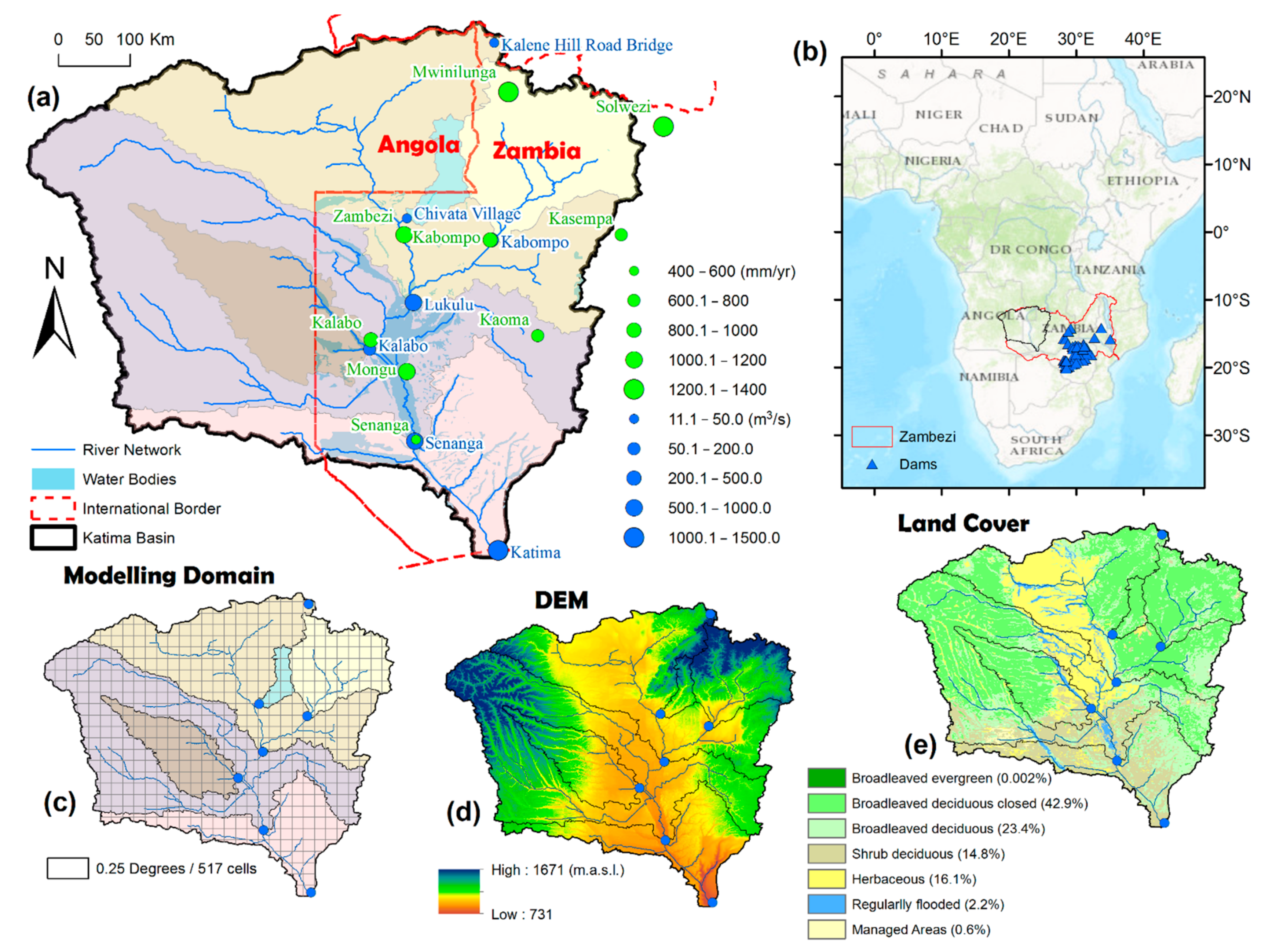
2.1. The Upper Zambezi River Basin (UZRB) Domain
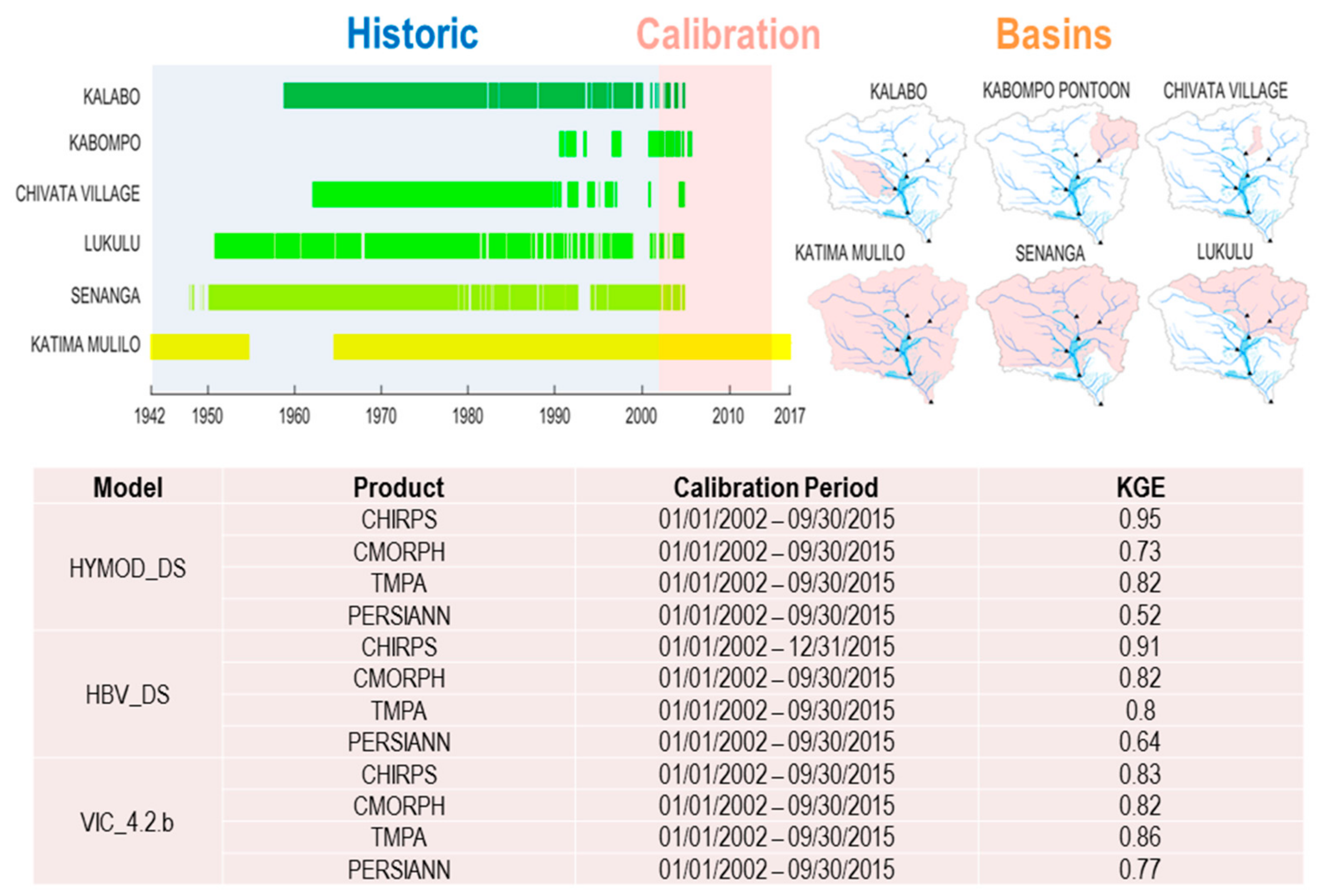
The operational HFS implementation for the UZRB and its sub-basins with records (Table 1), considered the drainage area (~339,521 km2) delineated above the Katima Mulilo streamgauge (Table 1 and Figure 1a). The mean annual streamflow at the UZRB (measured at Victoria Falls) represents about 25% of the mean annual streamflow measured at the Zambezi Delta outlet (~4200 m3/s), the largest contribution of all tributaries within the whole Zambezi Basin [23,24]. The historic mean daily flows (1942–2017) measured at Katima Mulilo stream gauge were about 1174 m3/s (Table 1); however, during extreme episodes the maximum daily streamflows can exceed more than six times the mean daily streamflows. The basin is dominated by broadleaved trees (~66%), herbaceous (16.1%), and shrubs (14.8%), whereas only a little (~0.6%) of the area is managed or represents agriculture (Figure 1c). The spatial distribution of these vegetation types is consistent with the elevational pattern of the basin, which ranges between approximately 731 and 1671 m above sea level (Figure 1d). The UZRB domain for the operational HFS implementation was set up using grid cells at 0.25° of spatial resolution, approximately 25 km at the Equator (Figure 1e). This area above Katima Mulilo was selected, because it is the unique portion of the Zambezi that does not have ongoing hydropower or water storage infrastructure projects (see Figure 1b). This is an advantage for HFS implementation since the presence of dams or any other anthropogenic water regulations can be an important limitation when the primary objective is to simulate natural streams.
Table 1. Description of streamgauges use in this study. The HFS column shows those streamgauges (sub-basins) used for the calibration of hydrologic models.
CountryStreamgaugeSouth LatitudeEast Longitude Area (km²)Altitude (m.a.s.l.)Average Flow (m3/s)PeriodMissing (%)HFS
ZambiaKalene Hill Road Bridge−11.1324.25764126112.31977–200434.81No
ZambiaChivata Village−13.3323.153354106517.41962–200423.32Yes
ZambiaLuanginga-Kalabo−14.9622.6834,621102159.01958–20048.94Yes
ZambiaKabompo Pontoon−13.6024.2142,7401029252.21990–200551.04Yes
ZambiaLukulu−14.3823.233206,5311012772.01950–200412.44Yes
ZambiaSenanga−16.1123.25284,538992972.61947–20048.40Yes
NamibiaKatima Mulilo−17.4824.3339,5217461174.51942–201713.54Yes

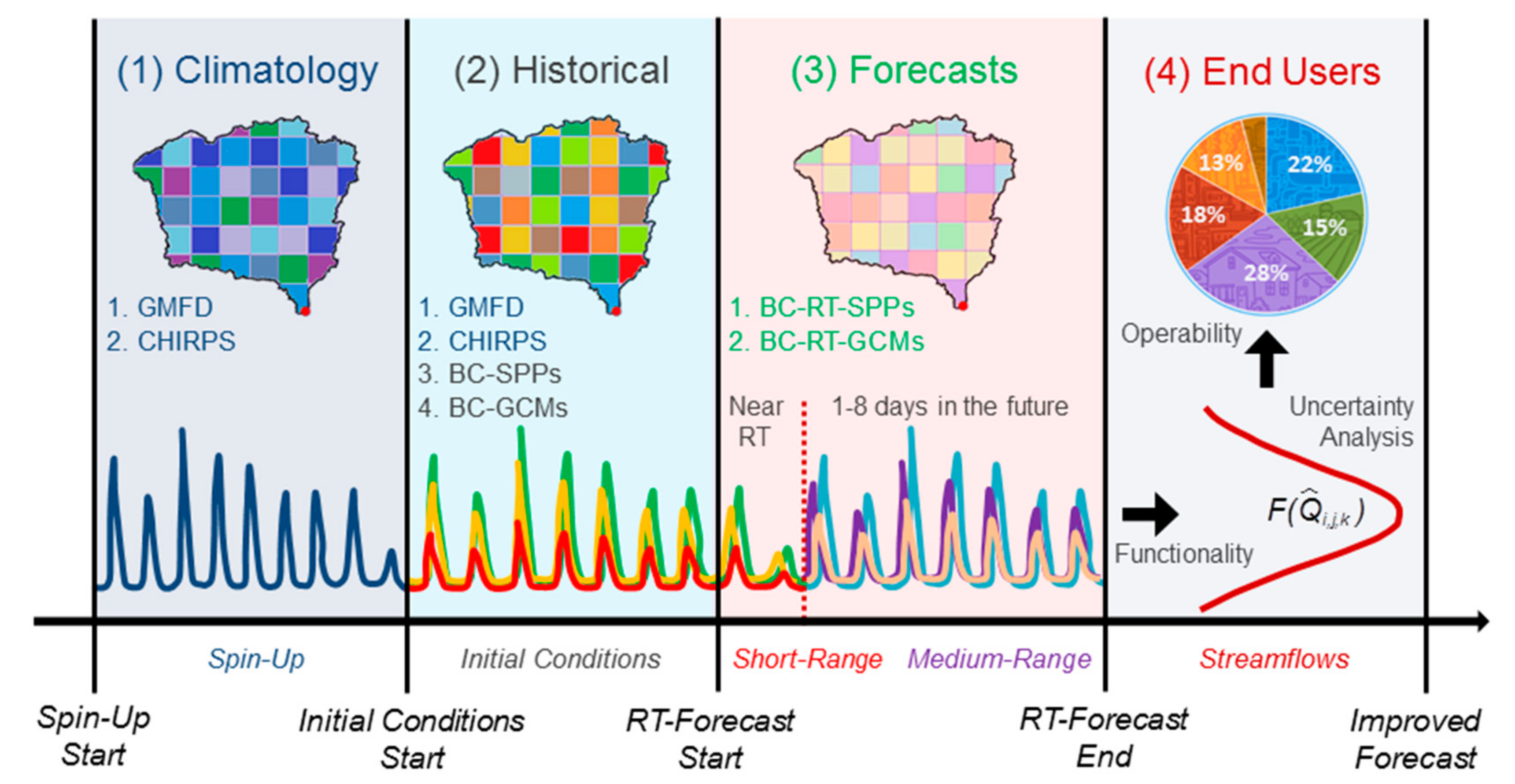
2.2. Forecasting Timescales and Water Management Activities

An HFS can be implemented for either of the three (or a combination thereof) principal forecasting timescales: (1) Realtime Monitoring or Short- to Medium-Range Forecasting (SR2MR), (2) Subseasonal to Seasonal or Short- to Long-Range Forecasting (SR2LR), or (3) Climate Change Predictions. The choice of forecasting timescales is partly determined by the relevant water management goals, and the needs of end users of the forecasts. In this study, the need for better water management schemes for flood warning and water allocation in the lower Zambezi Basin prompted the implementation of an HFS for realtime streamflow monitoring and short- to medium-range (SR2MR) forecasting in the UZRB and its sub-basins. As mentioned in the previous section, the HFS was implemented to forecast streamflow in the UZRB because it is the only part of the whole Zambezi River Basin without water regulation infrastructure, i.e., natural streamflow patterns can be observed in the UZRB. The SR2MR scheme allows streamflow forecasting from realtime up to eight days into the future (Figure 2).

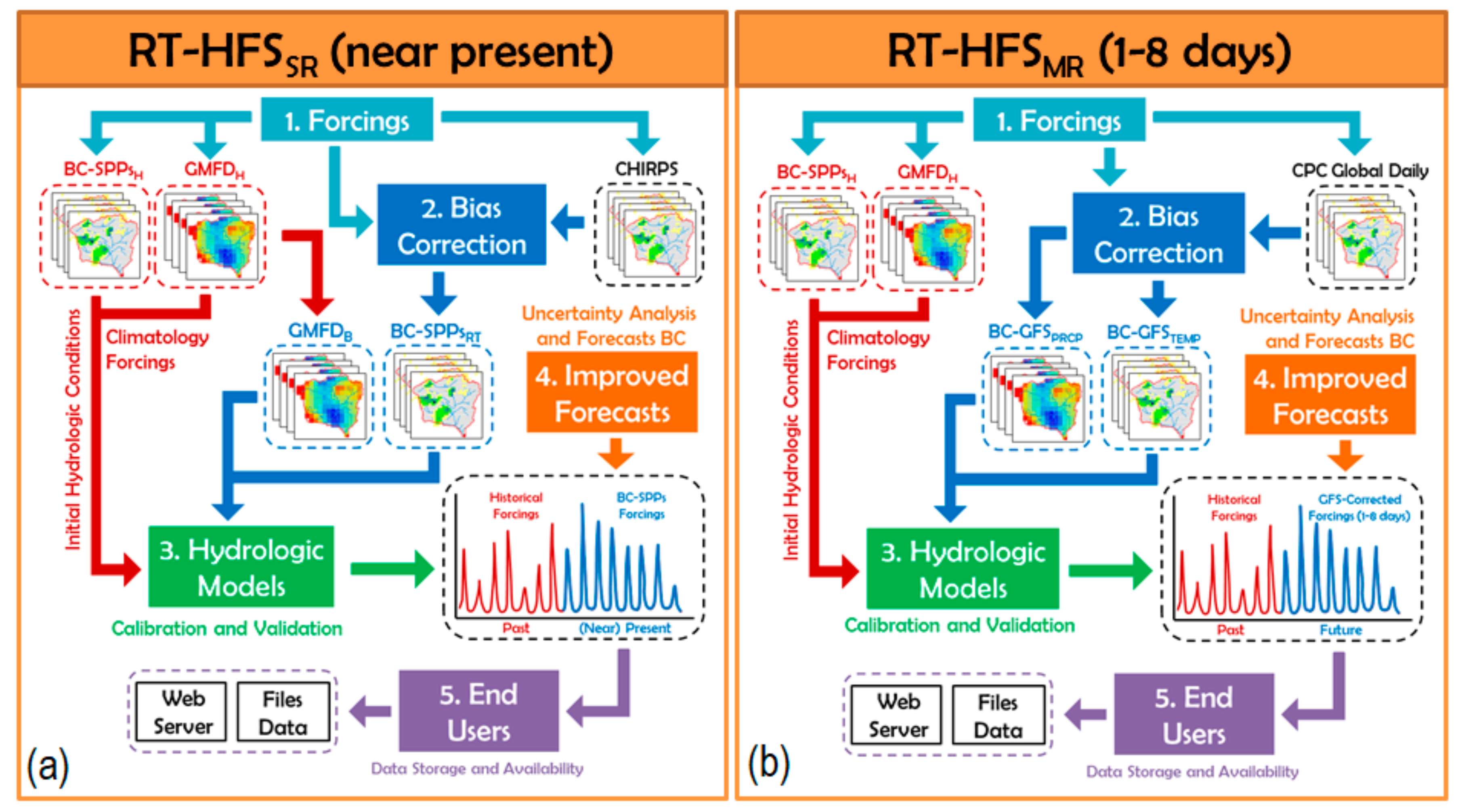
2.3. The Operational Context of a Hydrologic Modeling Paradigm

A functional HFS requires the design of a hydrologic modelling paradigm under an operational scheme. The design can range from a simple propagation of meteorological forecasts using a single hydrological model to more advanced techniques which can include multiparameter, multimodel, or multi-initialization schemes (Figure 3). The use of a simple propagation scheme does not allow for the quantification of the hydrological uncertainty propagated from the model structure or from the model parameters. However, by adding more parameter sets for a single hydrological model (i.e., [15]), by adding more hydrological models [13,14,16,17,18], or simply by performing more initializations of the initial starting conditions of a single model [19,20], the hydrological uncertainty either from the parameters, model assumptions, or initial conditions can be quantified.
In the UZRB, the operational HFS is designed as a VEF modelling paradigm [22] in which the best SR2MR forecasts are derived from the combination of multiple precipitation products, multiple hydrologic models, and multiple parameters sets (Figure 3). This technique makes it possible to increase the range of possible streamflow forecast ensembles that can be used to evaluate and select the best representations of the hydrological states and fluxes for the UZRB and its sub-basins.

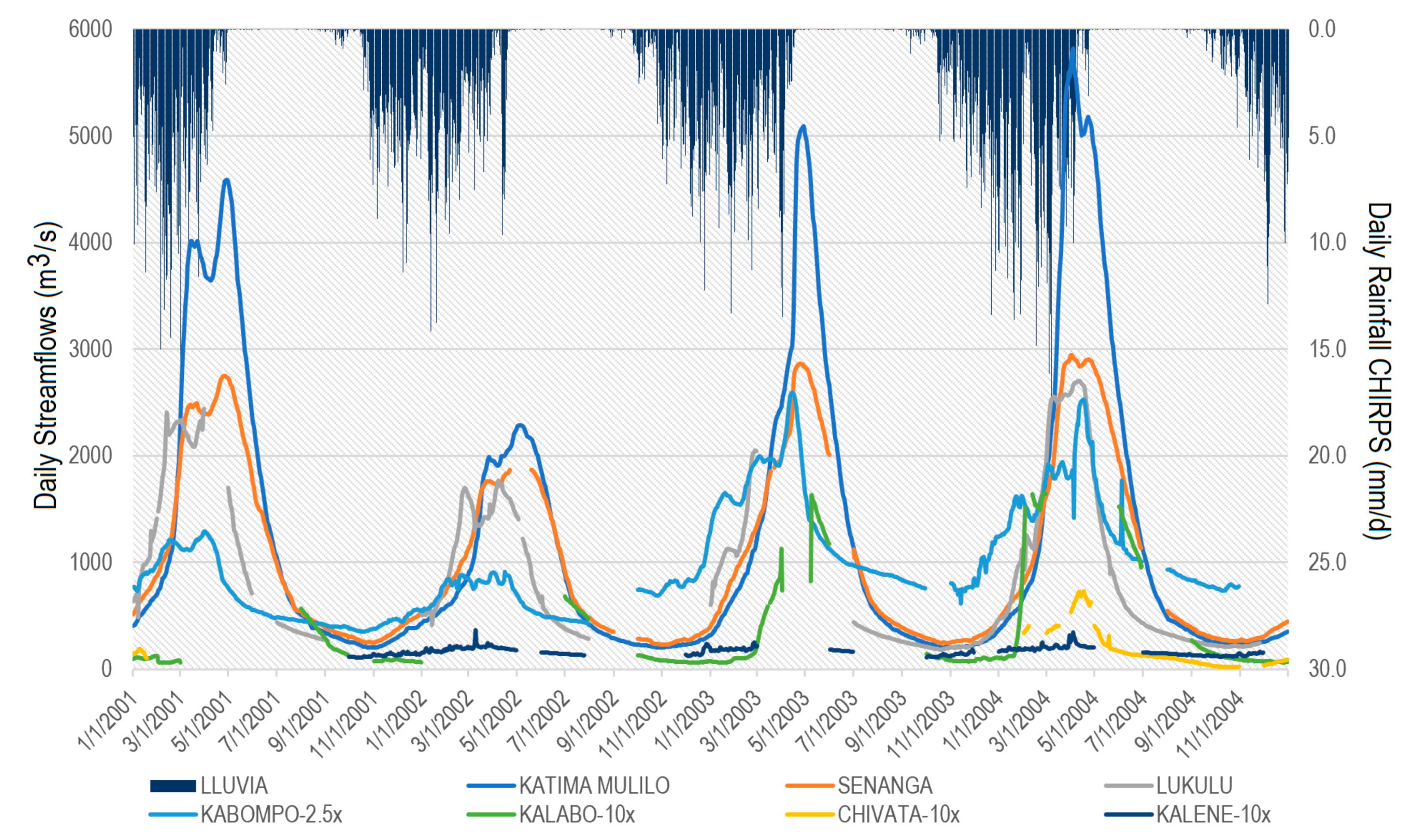
2.4. Selection of Hydro Climatological Forcings

The input data can have significant impacts on the propagation of meteorological and total hydrological uncertainty, and consequently, on the final streamflow forecasts. In this regard, it is well known that rainfall is the most important variable for streamflow simulation. At this stage, either point-based instrumental records or gridded-based climatology products can be used to establish baseline conditions and to correct SPPs or RCMs. The UZRB is a poorly gauged basin that lacks a consistent hydrometric network with continuous records (only nine rain gauges with discontinuous records were available for the HFS implementation). Therefore, the hydrological preprocessing hypothesis (also known as meteorological postprocessing hypothesis) [22] was approximated using rainfall climatology provided by CHIRPS (Climate Hazards Group InfraRed Precipitation with Station data) [25,26], and temperature climatology provided by the Global Meteorological Forcing Dataset (GMFD) [27].
To minimize the probability of errors propagated during the implementation of the operational HFS, the quality of the climatological forecast products used in an HFS needs to be evaluated and validated before they can be reliably used for hydrological applications. In the UZRB, three SPPs were evaluated, corrected, and then used to provide short-range (realtime) rainfall estimates (1) TMPA-RT [28]; (2) CMORPH [29]; and (3) PERSIANN [30,31]. To complete the SR2MR scheme, medium-range rainfall forecasts from the Global Forecasting System (GFS) [32] were used. The original GFS product provides rainfall forecasts in six-hour intervals (00, 06, 12, and 18 UTC) up to 16 days into the future. However, since the quantity of missing records between 9 and 16 days in the archives is larger (at least in this region), only rainfall forecasts provided at 00 UTC and up to eight days into the future were selected for operational implementation. (Table 2).

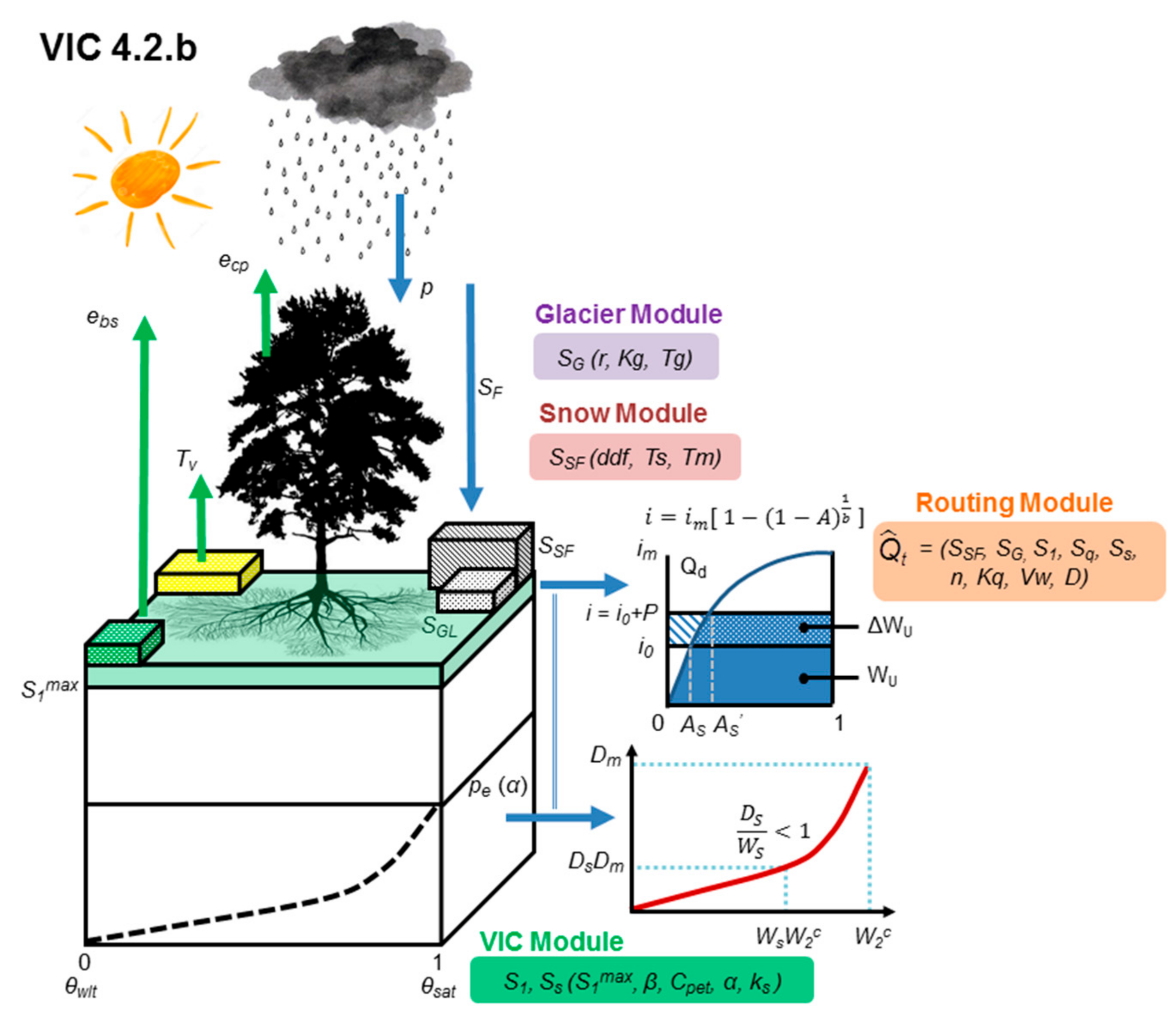
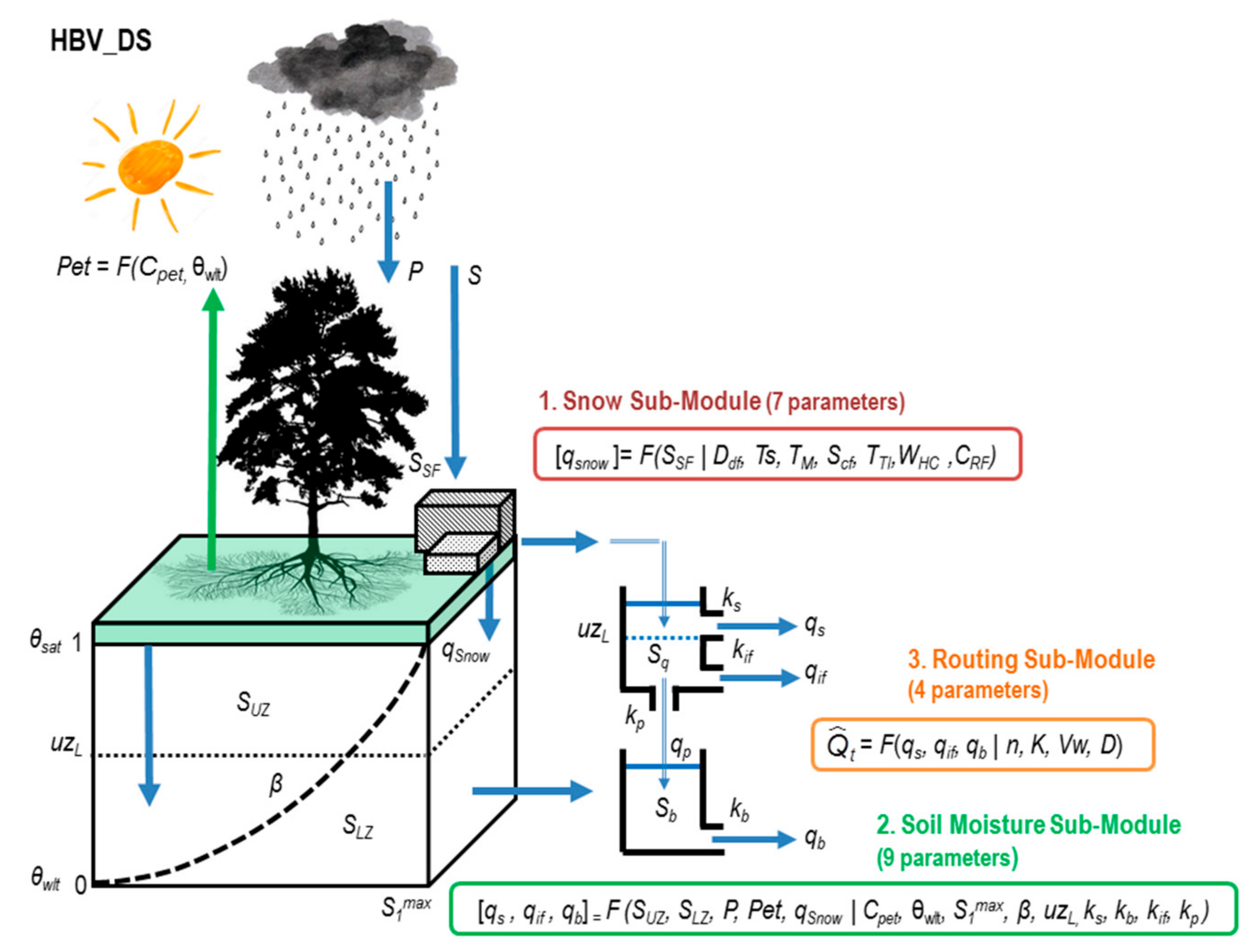
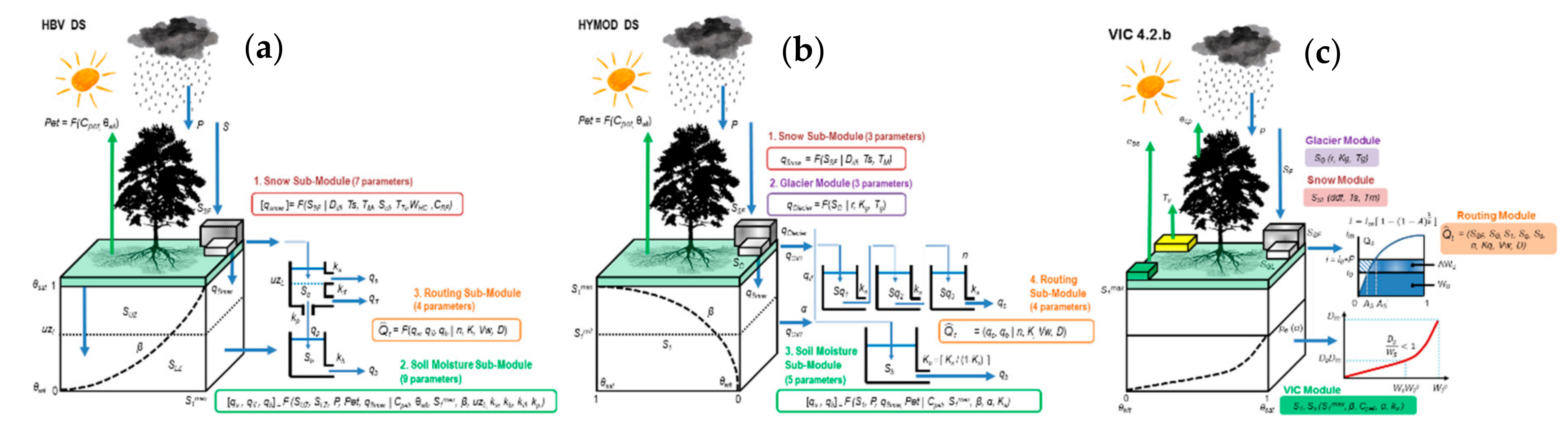
2.5. Hydrologic Models for Operational HFS

The selection of a model structure to be included in the hydrologic modelling paradigm (HMP) and ultimately in the operational HFS is as important as the selection of the model parameters to be used in the calibration process [16]. For an operational HFS, many HMP options can be implemented, including a single selection or an optimal combination of multiple precipitation or climate products, multiple hydrological models, multiple model state initializations, and/or multiple parameters sets. For example, the operational VEF approach implemented in the UZRB, and its sub-basins utilized three distributed hydrologic models (at 0.25° of spatial resolution): (1) HBV_DS, (2) HYMOD_DS, and (3) VIC 4.2.b (Figure 4). The first two models are distributed versions of two traditional well-known hydrological models: HBV [33,34] and HYMOD [35,36]. The VIC model used in this study is a modified version of the well-known Variable Infiltration Capacity (VIC) land surface model [37] that can resolve both the water and the energy balances. The modification allows postprocessing of VIC model outputs with the Lohmann’s model for routing [38]; a Gamma distribution to represent the catchment’s unit hydrograph; and the linearized version of the Saint-Venant Equations for final river routing. Additional details of the model states, fluxes, and parameters used in this study are provided in the Appendix A.

2.6. Calibration of Models Included in the HFS

The models described in the previous section were calibrated and validated for the whole UZRB and its sub-basins at 0.25 degrees of spatial resolution (approximately 25 km at the Equator). Historical available daily streamflow records for the UZRB and its sub-basins were used as reference data (Figure 5 and Figure 6). The genetic algorithm [39] was used to optimize the parameter sets of the three models. However, at this stage, any suitable optimization scheme can be implemented (e.g., [39,40,41,42,43]; and many others) based on the availability of time, resources, and expertise. In this study, a daily pooled calibration considering all observed daily records in the UZRB, and its sub-catchments (Figure 5) was applied at the Massachusetts Green High-Performance Computing Center (MGHPCC). The algorithm was run in parallel processing mode using 100,000 iterations, with population sizes ranging between 100 and 1000 generations. With this approach, the evaluation of the most appropriate population of parameter sets within each generation could be conducted in a more efficient manner. The Kling-Gupta efficiency [44] and the Nash-Sutcliffe efficiency [45], among other measures, were used to evaluate the degree of agreement between observed and simulated streamflow (Figure 6).

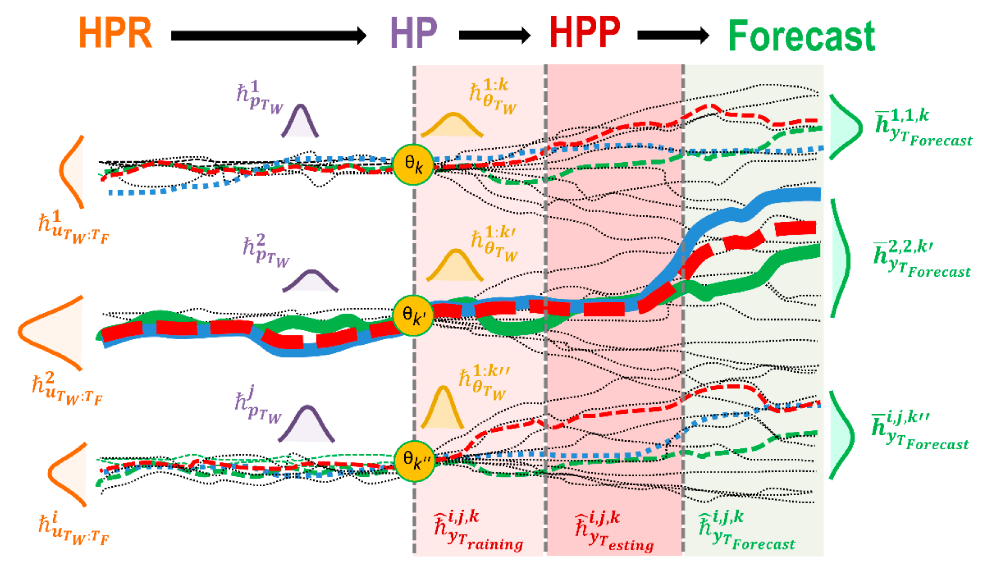
2.7. Operational Variational Ensemble Forecasting (VEF)

A group of i hydroclimatological inputs, j hydrologic models, and k calibrated model parameters can be used to establish simple or variational ensemble forecasts. A VEF approach can provide a larger number of forecasts than a simple assembling approach, because it evaluates all possible modelling chain sequences that can be arranged to construct an HFS (see Figure 7). At this stage, data assimilation techniques to support the “perfect model assumption” can be also applied to generate deterministic streamflow forecasts. Ref. [46] reviewed and evaluated many available methods to perform deterministic forecasts. However, in an operational context, the experience of streamflow forecasters suggests that uncertainty bands can better support decision making for water management schemes [47,48,49,50,51,52]. The intention of a VEF approach is to use all available weighted or non-weighted components of a modelling chain (HFS) to generate streamflow forecasts. The final hypothesis about the probability distribution of streamflow forecasts can be approximated using several procedures applied to the Multiproduct, Multimodel, and Multiparameter sets, through the implementation of a VEF approach that can be trained during TW and used during TF as:
( z y T F i , j , k | u T F i , p T W j , θ T W k ) = ( z y T F i , j , k | u T F i , p T W j , θ T W k )   T W t 0 , , t   and     T F t , , t f
u T F i = ( u T F i | z u T W i , z u T F i )
p T W j = ( S T W j | θ T W k )
θ T W k = ( θ T W k | z θ T W k )  
y T F i , j , k = ( z y T F i , j , k | u T F i , p T W j , θ T W k )
  • where, is a Multiproduct, Multimodel, and Multiparameter Variational Ensemble Streamflow Forecast for the forecast period TF.
  • is a family of hypothetical ensemble components for the warmup period TW and used to forecast the period TF.
  • y T F i , j , k is a hypothesis of the hydrologic process from a family of input data i, hydrologic model j, and parameter set k, about the HFS for the forecast period TF.
  • z y T F i , j , k is the streamflow prediction i, j, k about the HFS response for the forecast period TF.
  • u T F i is a hypothesis of the input data from a family of input data i about the HFS for the forecast period TF.
  • p T W j is a hypothesis of the hydrologic process from a family of hydrologic models j and for the warmup period TW.
  • θ T W k is a hypothesis of the parameter sets from a family of parameter sets k for the warmup period TW.
  • u T F i is the control variable for the forecast period TF.
  • z u T F i is a family of input data i about the HFS for the forecast period TF.
  • z u T W i is a family of input data i about the HFS for the warmup period TW.
  • S T W j is the model structure j for the warmup period TW.
  • θ T W k is the parameter set k for the warmup period TW.
  • z θ T W k is a family of parameter sets k for the warmup period TW.
The VEF approach (Figure 7) makes it possible to explicitly represent how different components of each model ensemble (modelling chain) vary according to all possible combinations of biogeophysical representations of the climate system and the hydrologic system (e.g., [53]). In addition, one of the novel aspects of this research is introduction of the assumption that the forecast skill of hydrologic models to represent underlying hydrologic processes can be better captured by assessing the generalization capabilities of multiple optimal parameters sets.

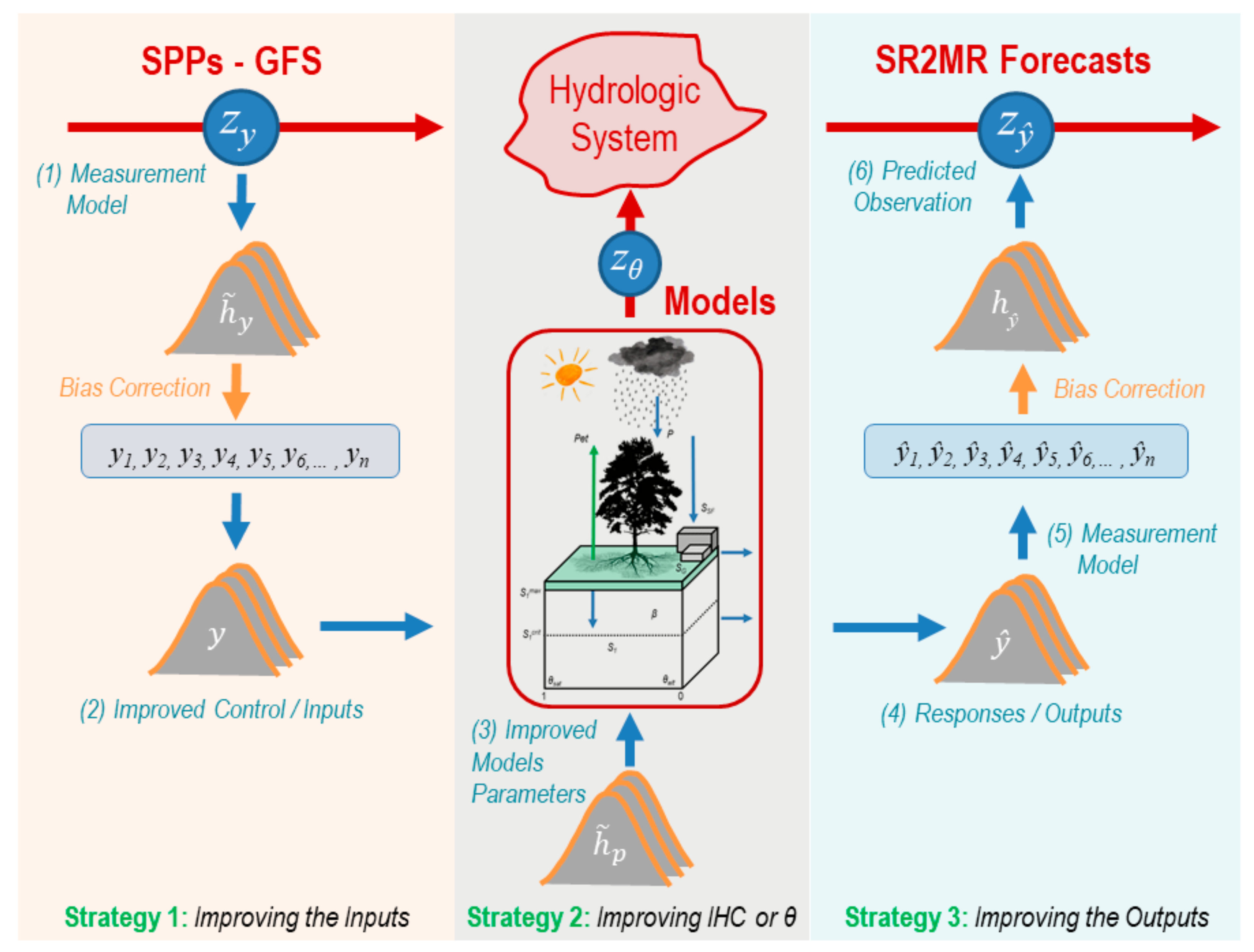
2.8. Strategies to Reduce Uncertainty and Improve VEF in an Operational Environment

In the development of an operational streamflow forecasting paradigm, it must be determined how total hydrological uncertainty will be reduced to improve streamflow forecasts. This topic is still a matter of discussion among many hydrologists and researchers around the world [47,48,49,50,51,52]. For instance, standardized processes to decompose, quantify, or evaluate the meteorological or the total hydrological uncertainty propagated from a modelling paradigm are required (see, i.e., Figure 8). The implementation of new techniques for the decomposition of uncertainty can take advantages from VEF approaches to explore all available sources of climate data and physical representations (i.e., model structures and parameters) for hydrologic modelling. Taking this into account, a combination of VEF and hydrological processing hypotheses can help us better understand how the propagation of errors occurs. For example, from multiple climate products the amount of meteorological uncertainty propagated through the modelling chain can be identified; then comparisons can be made to estimate the amount of total hydrological uncertainty (THU) propagated from the same system. This more systematic method to identify uncertainties can be useful to inform additional pre- or postprocessing of THU.
Assuming that an operational HFS can be evaluated as a VEF approach, three main strategies (Figure 8) to establish hydrological processing hypotheses can be applied to evaluate and improve the forecast skill of any hydrological model: (1) Hydrological Pre-processing (HPR) (or Meteorological Postprocessing), which can include the application of bias correction techniques (i.e., physical or statistical improvements) to reduce the propagation of errors or the application of Bayesian or non-Bayesian approaches to estimate an optimal weighted combination of precipitation products; (2) Hydrological Processing (HP), which can include improvements in the models’ structure, states, or parameters; and (3) Hydrological Postprocessing (HPP), which can include bias correction techniques applied over the streamflow forecasts or the use of Bayesian approaches to estimate an optimal weighted combination of streamflow forecasts.

3. Results

The three main strategies for the evaluation of hydrological hypotheses (HPR, HP, and HPR) were applied to evaluate and improve the forecast skill of operational streamflow forecasts in the UZRB. The implementation of one or another strategy can have significant impacts on the final forecasting products. For example, precipitation bias correction methods (HPR strategies) can dramatically perturb the volume of water entering to the system, in the HP strategies the most sensitive model parameters can significantly modify water routing though the model structure, and HPP strategies can have a large impact by directly perturbing the forecasts to adjust scaling and fitting issues derived from a poor model representation. Details on how these three processing strategies can impact operational streamflow forecasts are discussed in the following sections of this paper.

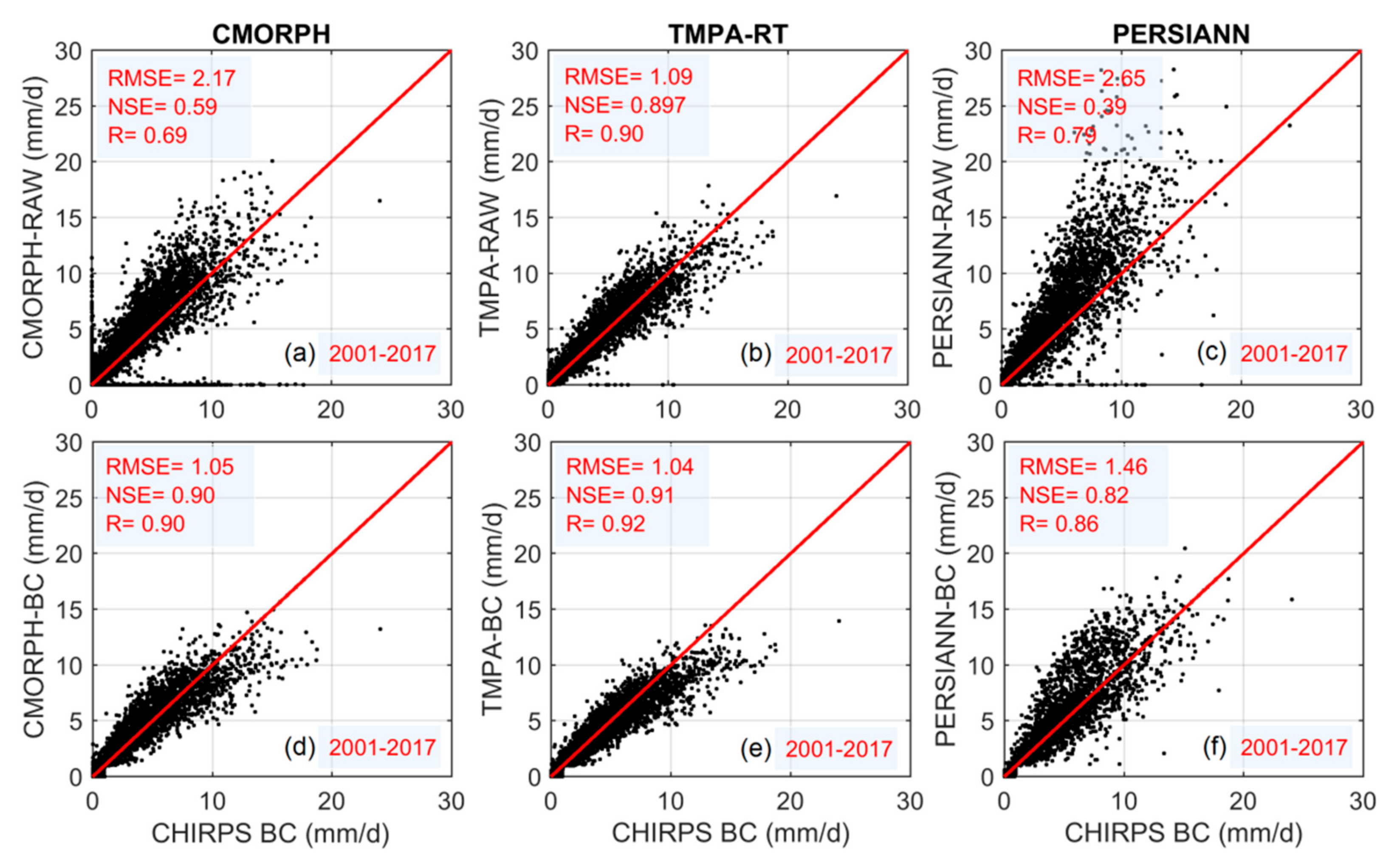
3.1. Strategy 1: Hydrological Pre-Processing (HPR)

Rainfall forecasts or any other climate forecasts derived from satellites or climatological models are prone to errors that must be corrected. The propagation of these errors is more significant when the forecasts are biased, especially those for rainfall, since this is the most important variable for hydrological modeling. Corrections applied over rainfall records allow for the identification of sensitivities or gaps associated to the improvement of satellite data, for the calibration and validation of variational hydrological models, and for the identification or selection of the best ensembles for any operational implementation of an HFS.
The corrections correspond to the application of any selected HPR hypothesis, and they contribute to the reductions of the propagated meteorological uncertainties through the VEF implementation. One of the most popular HPR strategies is Quantile Mapping [54,55,56,57], a technique that has been previously evaluated in the UZRB and compared to Principal Components Analysis (PCA) [13]. In the operational context, the Quantile Mapping (QM) technique is applied at a daily time scale with the assumption that the probability density functions (PDFs) of the rainfall observations and forecasts follow Gamma PDFs. The key idea behind this technique is to swap the quantiles of the simulated data with the quantiles of the observed data. The application of this technique has shown that daily estimates from SPPs and RCMs can be satisfactorily corrected at the catchment scale or at more regional scales (i.e., [54,55,56,57,58,59,60]). The previous studies agree with our findings for the UZRB where precipitation estimates from three satellites were significantly improved after the application of the Quantile Mapping (QM) method, used with a Gamma Probability Distribution Function (PDF). The results showed that all raw SPPs (Figure 9a–c) could be satisfactorily corrected at daily time scales (Figure 9d–f). Here, it is important to notice that many missing and false detections of rainfall can be corrected (see all raw to corrected scatters in Figure 9); however, the selection and fitting of a fixed PDF to the whole rainfall dataset can also reduce the performance of rainfall forecasts in some areas if (1) the selected PDF is not a good representation of the local climate conditions; if (2) the application of QM is exclusively tied to regional parameters instead of cell-by-cell parameters or vice versa, and if (3) only fixed temporal parameters are used instead of temporally varying parameters. All these factors can have result on successful or inadequate rainfall corrections that can have a significant impact on the next steps related to model calibration, final structural design, and generation of final operational streamflow forecasts products.

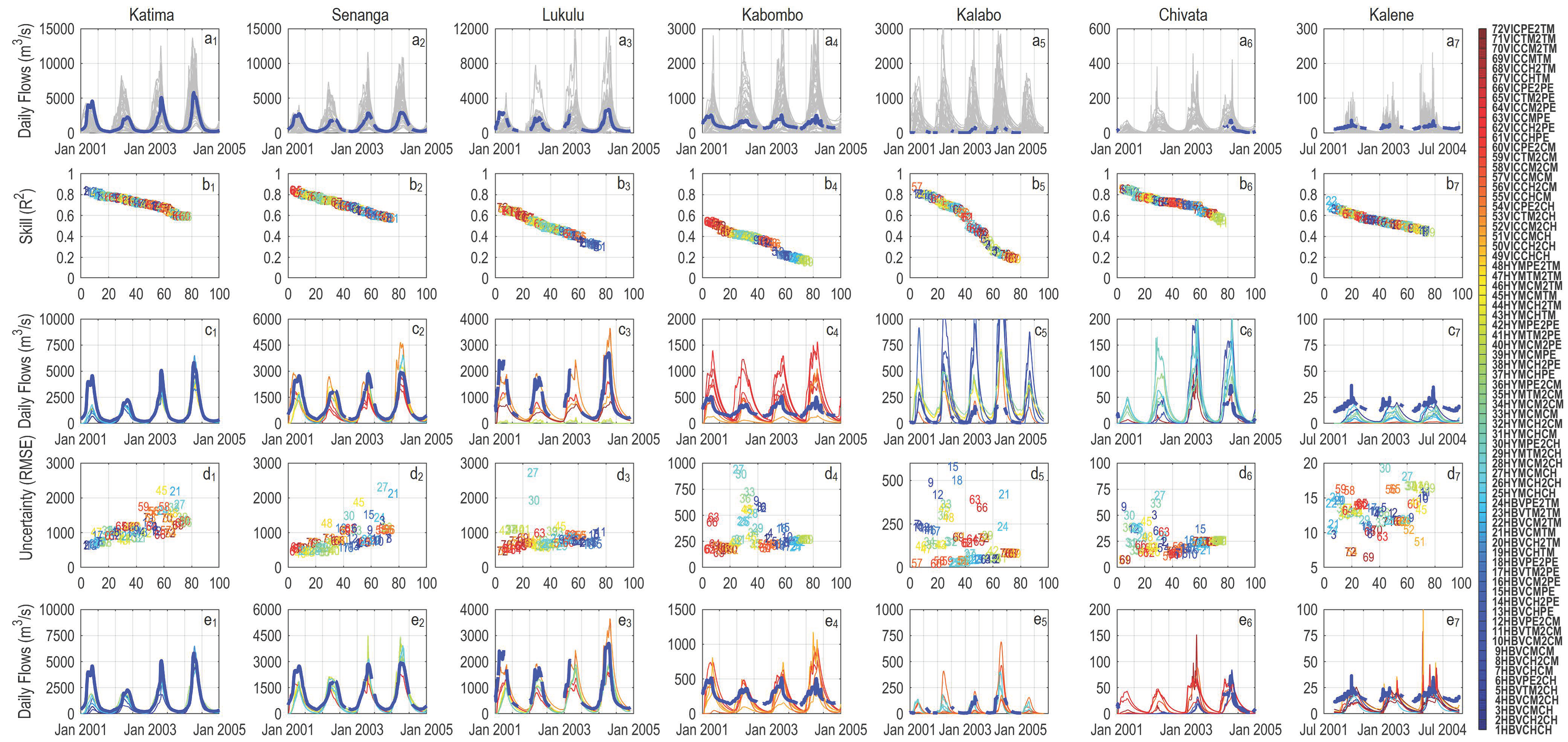
3.2. Strategy 2: Hydrological Processing (HP)

The VEF hydrologic modeling paradigm requires bridging science and engineering for the design of functional and operational HFS. Therefore, all available precipitation datasets utilized during HPR, must be used to evaluate the propagation of meteorological uncertainty into final SR2MR streamflow forecasts (see Figure 10a1–a7). Generally, the objective of HP is to constrain the range of valid model outcomes for the application of HPP strategies and for the generation of forecast products. Multimodel Ensemble approaches are a popular alternative to propagate uncertainty into future forecasts; however, they can yield boundless errors in inference, which can produce unbounded uncertainty bands [61]. Although this is an acceptable argument, the science and engineering of streamflow forecasting can play an important role in defining the best alternatives for the management of total hydrologic uncertainty (THU). In doing this, Variational Ensemble Forecasting (VEF) approaches have the advantage that they can be implemented using all available sources of input data, hydrologic models, and optimal parameter sets, to improve the assimilation of forecasts. VEF can also be coupled with regularization techniques to constrain the forecasting range based on the classification and evaluation of historic events to define the best ensembles for HPP.
Constraining and selecting the best ensembles for operational forecasting should be understood as a procedure that can vary at any model run. The variation of ensembles depends on the historic forecast skill performance estimated for all available hydrological events and their classified characteristic responses. In the UZRB and its sub-basins, the implementation of an operational VEF approach was used to generate SR2MR streamflow forecasts derived from all possible combinations of SPPs, hydrologic models, and optimal parameter sets (Figure 10a1–a7). The propagation of meteorological uncertainty can be quite large in the resulting streamflow traces when the whole input-model-parameter space is mapped and used for operational forecasts. To avoid unbounded uncertainty bands, the VEF approach allows improving the accuracy of streamflow forecasts through a ranking evaluation and posterior identification of the best hydrologic ensembles for the UZRB (Figure 10b1–b7 for forecasts ranked using skill analysis of R2 and Figure 10d1–d7 for forecasts ranked using total uncertainty defined as RMSE). Then the best ten raw streamflow forecasts are ranked using skill and/or uncertainty measures (Figure 10c1–c7,e7–e7). The application of specific or combined verification techniques on streamflow forecasts usually leads to an improvement of the HPP hypotheses. This multiple evaluation is helpful to identify how skill and uncertainty perform over space and time but also to evaluate how the spatial resolution of precipitation products can have a large effect on the operational forecasts. For instance, the smallest sub-basins inside the UZRB (see Kabombo, Kalabo, Chivata, and Kalene in Figure 10) resulted in higher total uncertainty compared to large basins (see Katima, Senanga, and Lukulu in Figure 10). This reduction in performance in the smallest sub-basins is probably associated with the smallest number of available precipitation grid cells, which produces larger averaged forecasting errors if missing or false detections are present in the forecasts.

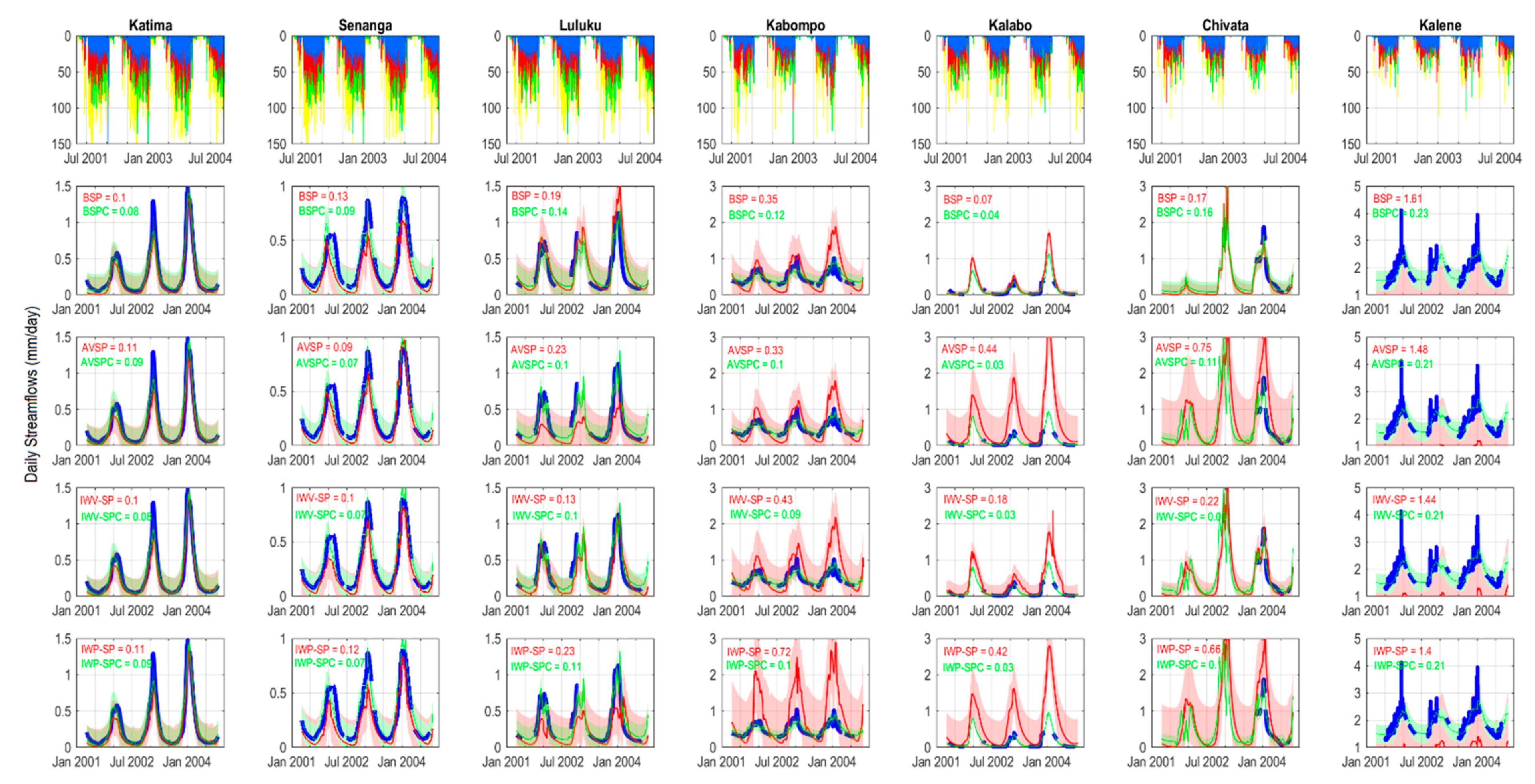
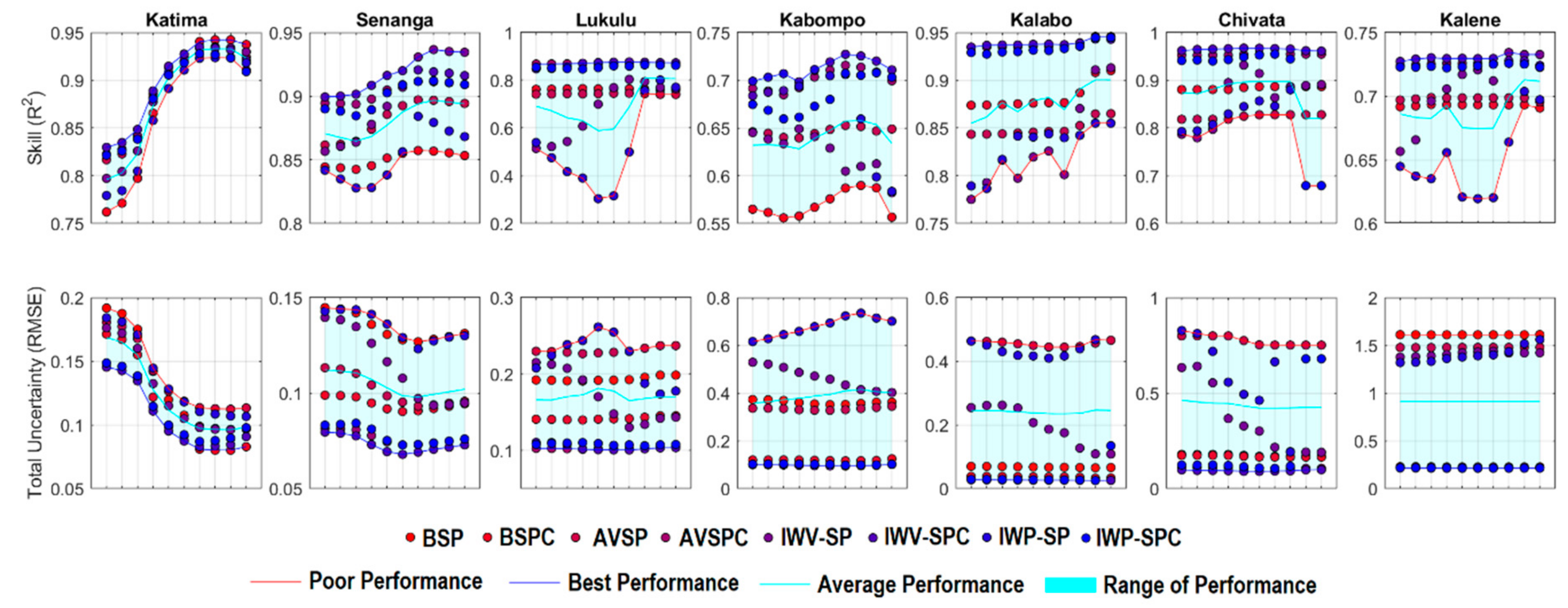
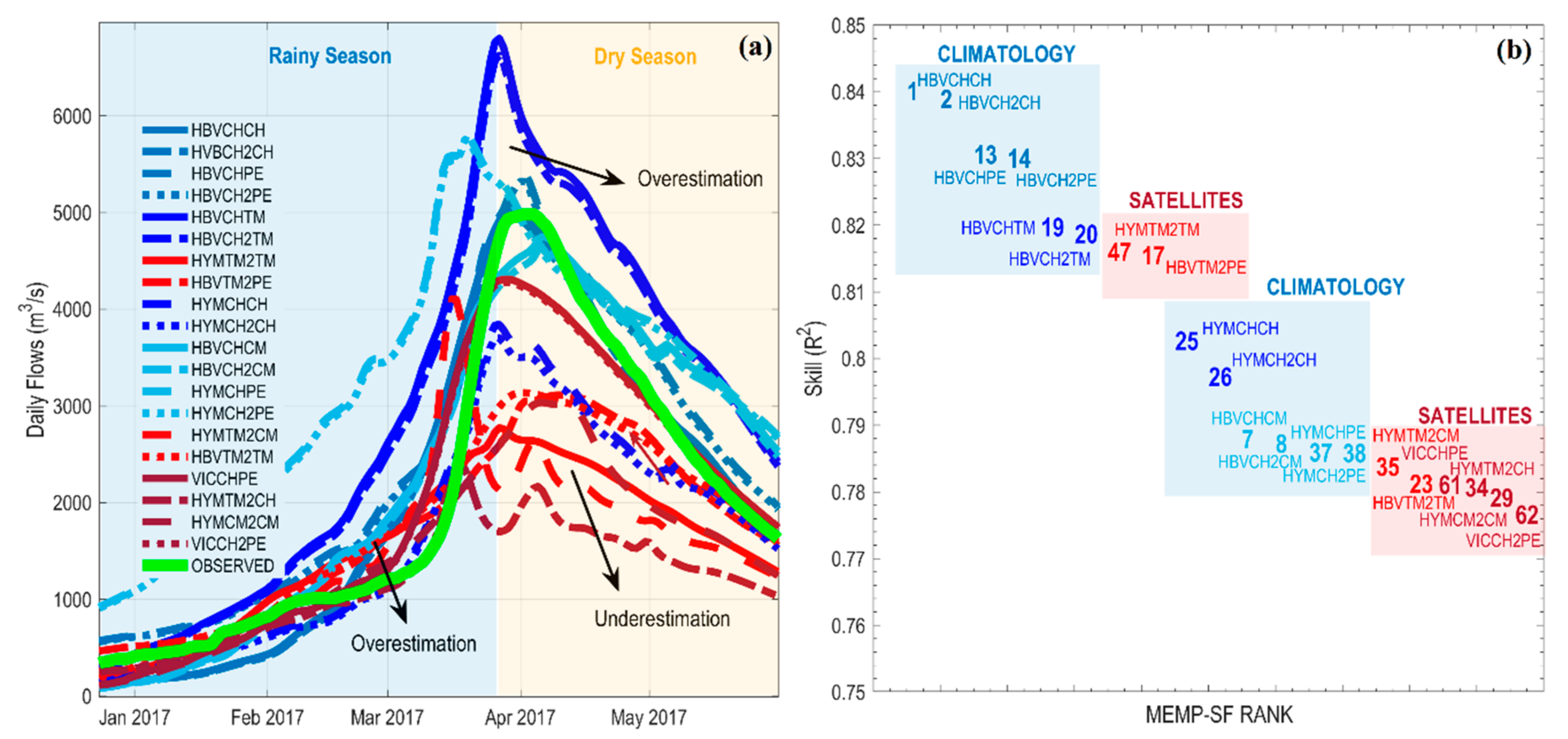
3.3. Evaluating Pre-Operational SR2MR Streamflow Forecasts

All 72 possible SR2MR forecasts that were generated in the UZRB by the combination of multiple rainfall products, hydrological models, and optimal parameter sets, enabled the identification of differences between the satellite precipitation products (SPPs) and their HPR strategies (or bias corrections) but also between the hydrological models and their optimal parameter sets (or HP strategy). From the VEF approach, the best raw model ensembles (Figure 10) were retained (20 out of 72 ensembles were selected for this study) and used for the generation of final streamflow forecasts products and reports for end users.
In general, an expected outcome is to have climatology products with better forecast skill (see for example Figure 11a,b) because of the instrumental corrections applied during the Hydrological Preprocessing (HPR) stage. However, one disadvantage of the climatology products is that they are not available in the SR2MR domain. For this reason, SPPs and RCMs are still needed for SR2MR streamflow forecasts in the UZRB or any other basins around the World. Therefore, the selection of final streamflow forecasts is also operationally based on SR2MR records. Furthermore, the quantification and propagation of retrospective meteorological uncertainties might be required for the release of final forecasts depending on the needs of end users. In the UZRB, multiples ensembles for deterministic streamflow forecasts and the spread of uncertainty by means of a probability density function were established for each daily SR2MR forecast. These forecasts were provided for Namibian Hydrological Services, one of the relevant African institutions that manages water resources in the Upper Zambezi River.

3.4. Strategy 3: Hydrologic Post-Processing (HPP) for Raw Streamflow Forecasts

Our inability to generate exact physical representations of natural hydrologic systems creates the need for streamflow forecasts that can quantify and reduce the total hydrologic uncertainty (THU) propagated from a hydrologic modelling paradigm (HMP). Hydrological Postprocessing (HPP) hypotheses focus on establishing standardized methods to quantify and propagate total hydrological uncertainty (which is the sum of all uncertainties i.e., input, parameter, or structural uncertainties propagated into the final streamflow forecasts). Similar to HPR and HP, different methods can be applied for HPP hypotheses, i.e., stochastic, Bayesian, or machine learning methods can be used as post-processors for the final ensemble of SR2MR streamflow forecasts. The objective at this stage is to minimize the error of the deterministic forecast but also the spread of total hydrological uncertainty around the raw streamflow forecasts. The deterministic forecast can be obtained as an optimal weighted SR2MR streamflow forecast, which is used to propagate the total hydrological uncertainty (Figure 12). In the UZRB, a Multivariate Combinatorial Linear Regression (MCLR) approach was applied as a regularization technique to inform the best selection of hydrologic ensembles that minimized the spread of total hydrologic uncertainty. The MCLR was also used as a first level hydrologic postprocessor to resolve scaling issues of the raw streamflow forecasts (Figure 12). The final ensemble of raw and corrected SR2MR streamflow forecasts was then evaluated using two inference-based hydrologic postprocessors: (1) Inverse-Variance Weighting (IVW), and (2) Inverse-Probability Weighting (Figure 12). Both approaches were compared to the best streamflow prediction (BSP) and the Average Streamflow Prediction (AVSP) using the retrospective total hydrologic uncertainty quantified using the root mean square error in millimeters per day (Figure 12). The application of hydrologic postprocessors (MCLR, IVW, and IWP) revealed an improved efficiency of both the forecasts and the propagation of THU in the UZRB and its sub-basins (Figure 12).
The combination of HPP with short and long-term memory windows (for periods ranging between 5 and 180 days before the event) also proved to be more efficient in improving the performance of SR2MR streamflow forecasts (see Appendix A Figure A3 for details). The effect of HP for operational streamflow forecasting was mainly observed in two aspects: (1) a better performance of the deterministic streamflow forecasts, i.e., correction of scaling issues, and (2) narrower total hydrologic uncertainty bands around the deterministic forecast, i.e., more practical and realistic uncertainty bands for decision makers (see details in Figure 12).

4. Discussion

To establish operational hydrological forecasting systems (HFS) it is important to first define who will be the main and potential end users of the streamflow forecasts products within the basin under consideration. In the UZRB (Figure 1), the need for better water management schemes for flood warning and water allocation schemes has required the generation of daily SR2MR streamflow forecasts (Figure 2). Several water users and water authorities of the countries sharing waters from the UZRB can take advantage of the benefits of this operational HFS implementation, which can largely help developing sustainable water management and allocation activities for this transnational basin. For example, the water users of streamflow forecasts in the UZRB can be informed about the main water management decisions that need to be taken care of for water supply, reservoir management, hydraulic design, etc. These decisions are generally complex; therefore, under such a scenario, the best way to inform the local authorities and end users in the UZRB can be obtained if we had ‘perfect’ weather forecasts, or climatic predictions, that could be combined with ‘perfect’ hydrologic models to generate “almost” perfect streamflow forecasts. If this hypothesis were still true only one weather or climatic prediction (model), and one hydrologic model would be needed for streamflow forecasting. For example, the ‘perfect’ climate estimates of the climate model could be combined with one ‘perfect’ hydrological model, and the streamflow prediction should be close enough to inform both managers and users, so they can apply the right decisions for water management. The problem of this hypothesis is the fact that so far, hydrologists and meteorologists has not been able to create or establish perfect model representations of climate and hydrology, i.e., models are simplified representations of the hydroclimatological processes occurring across spatiotemporal scales. Therefore, we know and assume that during the operational implementation of the HFS in the UZRB there were countless sources of uncertainty, and different tools and schemes were established in this study to quantify how meteorological and hydrological uncertainty propagate through an operational VEF approach. One of the first adopted techniques that emerged was the utilization of single model realizations as those provided in many previous studies (see for example [3,4,5,6,7,8,9,10,11,12]). Then, multi-ensembles of climate predictions were used to quantify and propagate the meteorological uncertainty through the streamflow forecasts. The main issue of this technique is that it did not allow quantifying the uncertainty propagated from the hydrological model either from the model structure or from its parameters. To resolve this problem [15], proposed a way to quantify the hydrological uncertainty from a single model with multiple parameters that can be obtained from the calibration of multiple climate products. The final set of outputs is obtained from a multiproduct and multiparameter scheme. This technique allows quantifying the hydrological uncertainty propagated from multiple parameters sets of a single hydrological model; however, it does not allow quantifying how the uncertainty propagates and varies as a function of the structure of the selected hydrological model. This latter conceptualization of hydrological uncertainty is tied to the modelling assumptions required to establish the physical representation of the hydrologic system. Obviously, these assumptions also vary as a function of the selected hydrological model and its structure. In this context, hydrologists have opted to promote more comprehensive modelling schemes that combine multiproducts and multiple hydrological models [14,16,17,18]. With this technique, it has been possible to quantify the meteorological uncertainty propagated from the climate products and the hydrological uncertainty propagated from the hydrologic models and their corresponding structures. On the other hand, recent studies [62,63,64] have argued that the performance of a single hydrological model can be improved together with the streamflow forecasts if multiple climate products are combined with a model that is perturbed by generating multiple initializations with different initial conditions, i.e., changes in surface storage, groundwater storage, or snow storage, among others. The main objective behind this approach is to capture the current hydrologic condition of a catchment to assimilate streamflow. For example, in this regard it has been traditionally assumed that the warmup period is required for hydrologic modelling; however, this approach can be bypassed given that the initial states are adjusted beforehand, taking in consideration the streamflow assimilation. This scheme has also stablished a new source for the quantification of hydrologic uncertainty just by changing the initial conditions of the hydrological model. With this technique, a new research niche has been recognized by hydrologists and now is also applied to quantify total hydrological uncertainty (THU). Having said that, it is also important to add that all the schemes mentioned above have allowed quantifying the hydrological uncertainty in separated procedures, either from multiple climate products, from multiple hydrological models, from multiple parameters sets, or from multiple initializations. In fact, all these hydrologic modeling paradigms (HMP) are still applied in a systematic manner to identify and quantify different sources of hydrological uncertainty.
Despite the existence of all these HMP previously mentioned, none of them have proposed a combined technique to quantify both meteorological and hydrological uncertainties propagated from different sources of a VEF implementation (see Figure 7 and Figure 8), i.e., sources as climate forecasts, modelling assumptions, and optimal parameter sets, that can be evaluated for any operational hydrological forecasting system (HFS) implementation with VEF. To accomplish this issue, we have implemented a VEF approach [22] based on multiple satellite precipitation products (and GFS precipitation forecasts), multiple hydrologic models, and multiple optimal parameters sets for SR2MR daily streamflow forecasting. The VEF approach implemented in the UZRB (Figure 10) has allowed increasing the number of possible hydrologic ensembles available for streamflow forecasting, together with an improvement of the streamflow assimilation (observed versus predicted). It also provides a more comprehensive and systematic framework to identify and propagate the spread of total hydrologic uncertainty in an operational hydrologic forecasting system. Now, the natural question is how much room is left to define new modelling paradigms or techniques that can be used to quantify or minimize the propagation of total hydrological uncertainty? To answer this question, we need to differentiate between what we can do to define the best integrated implementation of an HFS, and what adjustments are required at each separated component (i.e., inputs, models, or outputs) of the HFS. The operational HFS implementation in the UZRB, identified and considered three general hydrologic processing strategies (HPS) that can be applied to any VEF approach. If we consider that any hydrologic modelling paradigm (HMP) can either include multiple inputs; hydrologic models, parameters, initializations; and outputs, then, we can hypothesize that at each component of the HMP it is possible to apply additional techniques or methods to improve streamflow forecasting. These strategies were conceptualized as: (1) Hydrological Preprocessing (HPR), (2) Hydrological Processing (HP), and (3) Hydrological Postprocessing (HPP). Taking advantage of the strategies proposed for the establishment of hydrologic processing strategies or hypotheses, standardized methods for HPR (Figure 9) and HPP (Figure 12) were applied in the UZRB, showing that the performance of raw VEF streamflow forecasts can be significantly improved, and the spread of uncertainty can be better constrained by applying regularization processes that combine the strength of Multivariate Combinatorial Linear Regression (MCLR) and Inference-Based approaches (Figure 12).
The science and engineering of future operational streamflow forecasting in the UZRB will continue concentrating efforts in improving the forecasts; however, new needs from end users might also require improving the physical representation at the catchment scale. For this, it will be necessary to establish the role of mathematical, statistical, and/or machine learning methods that can be used to correct and propagate the hydrologic uncertainty from different components of a VEF approach, i.e., Bayesian, stochastic, pattern, or inference-based learning methods, etc. The performance of different rainfall products and methods also needs to be evaluated across different catchment sizes and forecast timescales to determine the space–time variability that propagates total hydrologic uncertainty. This evaluation must also be extended to determine the dependence of the accuracy of the streamflow forecasts and the propagation of hydrological uncertainty from physically based models. All the above will indicate the applicability limits of the VEF approach based on multiple precipitation or climate products, multiple hydrologic models, and multiple optimal parameters sets. All of the above will allow the establishment of new robust theoretical and hypothetical paradigms to quantify, evaluate, reduce, and manage the propagation of total hydrologic uncertainty using VEF approaches.

5. Conclusions

This paper described the main stages and processes required to implement and improve an operational hydrologic forecasting system (HFS) in the UZRB and its sub-basins. The process of implementation is very complex, and important decisions needed to be made about the input data (precipitation from satellites or climate products), the hydrologic models to be included along with their optimal parameter sets, and the timescales required for the generation of streamflow forecasts.
Once the HFS was completely operational in the UZRB, additional improvements to the forecasts were required to improve its performance and reduce the spread of total hydrologic uncertainty into the final streamflow forecast products. In this regard, three general strategies to improve the performance of VEF approach were proposed: from Hydrological Preprocessing to Postprocessing techniques that can improve the input data, the hydrologic models (or their structures), the optimal parameter sets, and the raw streamflow forecasts. The whole range of available techniques for operational HFS will require more detailed and standardized conceptualizations. In this regard, bias corrections or preprocessing (HPR) techniques applied over the input data will still play an important role in operational hydrological forecasts for the UZRB. The operational implementation of the VEF combined with regularization and inference-based methods improved the performance of streamflow forecasts as the primary need from end users in the UZRB; however, new alternatives to improve the physical understanding of the basin are still a pending task. Finally, it is important to add that the science of Hydrological Postprocessing is still under an early stage of development, and it still lacks the standardized methods that can be used for these purposes. Emerging methods will need to be evaluated to establish the real boundary between physical and statistical needs in operational streamflow forecasting. This discipline will also require a natural merging of science and engineering (practical applications) in a real-world context to establish baseline conditions for streamflow forecasting and hydrological uncertainty quantification and propagation.

Author Contributions

Conceptualization, R.V.-P. and J.B.V.; methodology, R.V.-P.; software, R.V.-P., S.W. and T.R.; validation, J.B.V. and A.S.-C.; formal analysis, R.V.-P.; investigation, R.V.-P.; resources, J.B.V., A.S.-C. and S.W.; data curation, R.V.-P.; writing—original draft preparation, R.V.-P.; writing—review and editing, R.V.-P., J.B.V., T.R., S.W. and A.S.-C.; visualization, R.V.-P.; supervision, J.B.V.; project administration, A.S.-C.; funding acquisition, J.B.V. and A.S.-C. All authors have read and agreed to the published version of the manuscript.

Funding

This research was supported by NASA-USAID SERVIR Program, Award 11-SERVIR11-58.

Acknowledgments

This research was supported by the NASA-USAID SERVIR Program (Award 11-SERVIR11-58). The first author of this paper was supported by the National Research and Development Agency of Chile (ANID), through the National Doctoral Degree Scholarship Competition of the Formation of Advanced Human Capital Program. The Research Computing Department at the University of Massachusetts provided support on the calibration of the hydrological models. All these contributions are gratefully acknowledged.

Conflicts of Interest

The authors declare no conflict of interest.

Appendix A. Hydrologic Models Used for SR2MR Streamflow Forecasting in the UZRB
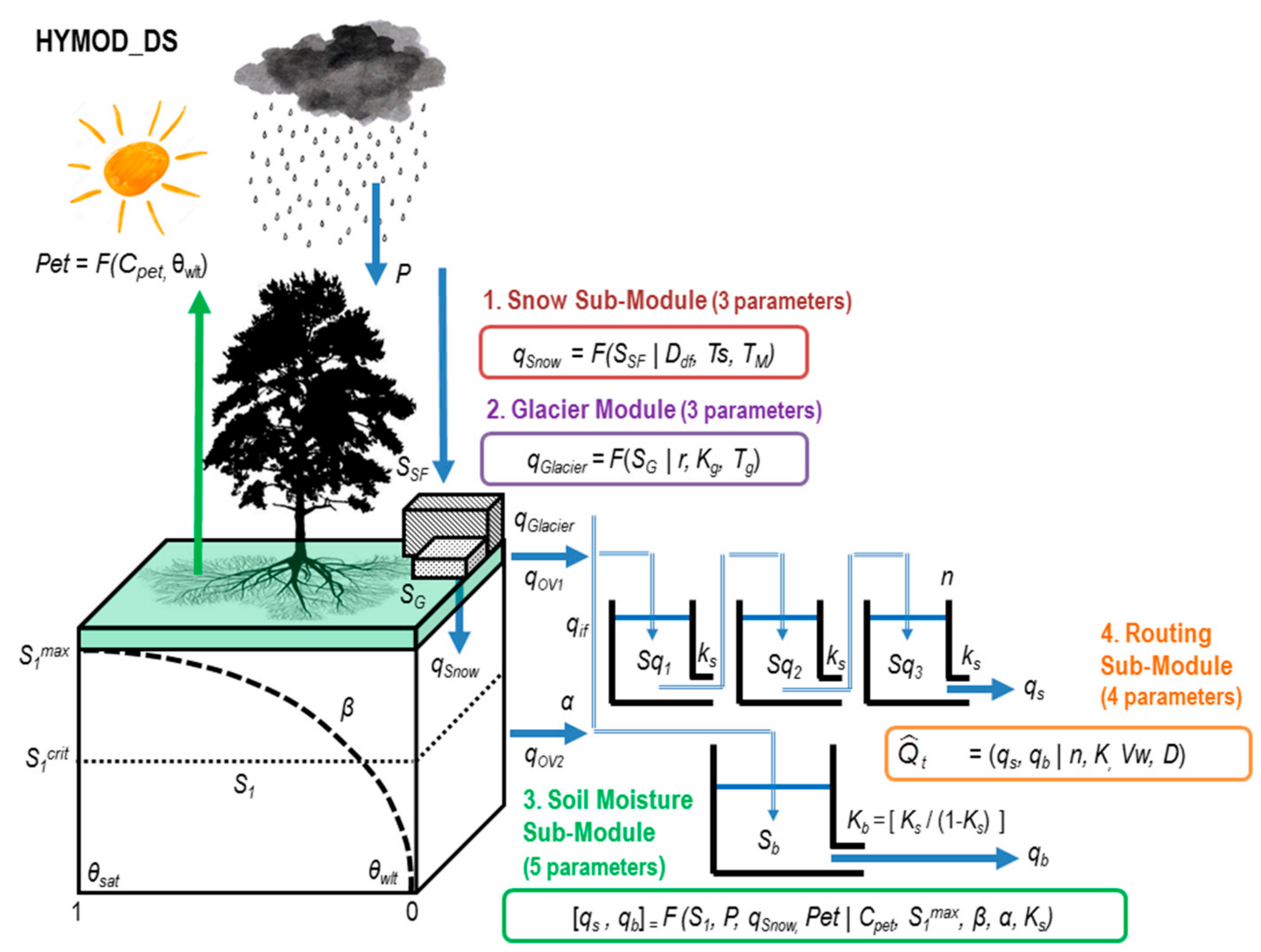
The HBV_DS model is a modified distributed version of the Hydrologiska Byrans Vattenbalansavdelning (HBV) model (see details in Bergström, 1976; Seibert and Vis, 2012; Yang and Wi, 2018), and it simulates catchment discharge on a daily time step, based on time series of precipitation and air temperature. The implementation of HBV_DS (Figure A1) requires the calibration of 20 parameters (see Table A1). The Potential Evapotranspiration (PET) is computed as a function of daily mean temperature and hours of daylight using the Hamon Method (Hamon, 1961). In the snow routine, the snow accumulation and snowmelt are computed by a degree-day method (see Moore, 1993; Rango and Martinec, 1995). The actual evaporation and the groundwater recharge are simulated as a function of the actual soil water storage. The surface runoff, the interflow, and the percolation are simulated using a single linear reservoir with three outlets, and the groundwater routing is represented by a single linear reservoir. The sum of these outflows is then routed using the diffusive wave approximation of the linearized Saint-Venant equation (Lohmann et al., 1998).
Figure A1. Hydrologiska Byrans Vattenbalansavdelning (HBV) Model Structure (states, fluxes, and parameters).
Hydrology 08 00188 g0a1
The HYMOD_DS model (Wi et al., 2015) is a modified version of the original HyMod Hydrological Model (see details in Moore, 1985; Boyle et al., 2000; Gonzalez-Leiva et al., 2016; Valdés-Pineda et al., 2016). The modified distributed version (Figure A2) simulates streamflows on a daily time step and requires daily precipitation and mean temperature as input variables. The implementation of HYMOD_DS requires the calibration of 15 parameters (see Table A1). The model is based on the probability-distributed storage capacity concept (proposed by Moore, 1985) to represent the soil moisture accounting component. Estimates of potential evaporation rates are calculated using the Hamon Method (Hamon, 1961). The rate of change in snow and glacier volume is expressed by the degree day factor (DDF) mass balance model (see Moore, 1993; Stahl et al., 2008). The direct runoff is characterized by an instantaneous unit hydrograph (IUH) (Nash, 1957), in which the catchment is represented as a series of “n” linear reservoirs. The groundwater routing is simplified as a single linear reservoir. Finally, similar to the HBV_DS model, the transport of water in the channel system is described using the diffusive wave approximation of the linearized Saint-Venant equation (Lohmann et al., 1998).
Figure A2. HyMod Hydrologic Model Structure (states, fluxes, and parameters).
Hydrology 08 00188 g0a2
The VIC (Variable Infiltration Capacity) Model (Liang et al., 1994, 1996; Cherkauer et al., 2003; Bowling et al., 2004; Bowling and Lettenmaier, 2009) is a large-scale semi-distributed hydrologic model (Figure A3). VIC simulates streamflows on a sub-daily or daily time step and requires daily precipitation, mean daily temperature, and/or mean wind speed as input variables. The VIC model has about 50 parameters; however, its implementation requires the calibration of 5 parameters (Table A1). The model balances both the water and surface energy budgets within the grid cell; and its sub-grid variations are captured statistically. The total evapotranspiration over a grid cell is computed as the sum of three types of evaporation: evaporation from the canopy layer of each vegetation tile, transpiration from each of the vegetation tiles, and evaporation from the bare soil (Liang et al. 1994). The snow model in VIC represents the snowpack as a two-layer medium and solves for energy and mass balance for the ground surface snowpack in a manner similar to other cold land processes models (Anderson, 1976; Wigmosta et al., 1994; Tarboton et al., 1995). The VIC model uses the variable infiltration curve (Zhao et al., 1980) to account for the spatial heterogeneity of runoff generation. It assumes that surface runoff from the upper two soil layers is generated by those areas for which precipitation, when added to soil moisture storage at the end of the previous time step, exceeds the storage capacity of the soil. The formulation of subsurface runoff follows the Arno model conceptualization (Franchini and Pacciani, 1991; Todini, 1996). To finally simulate streamflow, VIC results are postprocessed with a separate routing model (Lohmann, et al., 1996; 1998a; b), based on a linear transfer function to simulate the streamflow.
Figure A3. Variable Infiltration Capacity (VIC) Model Structure (states, fluxes, and parameters).
Hydrology 08 00188 g0a3
Table A1. Parameters included in the calibration of the HBV_DS, HYMOD_DS, and VIC models.
ModuleParametersDescriptionRangeUnitsModel
Soil MoistureCpetProportionality Coefficient of Hamon Potential Evapotranspiration0.1–2non-dimHVB–HYMOD
S1maxMaximum storage capacity of soil moisture accounting tank5–1500(mm)HVB–HYMOD
βShape parameter of the storage capacity distribution function0.01–1.99non-dimHVB–HYMOD
αSplit parameter for quick and slow components0.01–0.99non-dimHYMOD
θwltSoil Permanent Wilting Point (limiting soil moisture for PET occurrence)0.1–1non-dimHBV
uzLUpper reservoir water level for quick runoff occurrence0–1000mmHBV
KsRecession constant for quickflow in the upper reservoir0.01–0.99day−1HVB–HYMOD
KbRecession constant for slowflow in the lower reservoir0.0001–0.99day−1HVB–HYMOD
KifRecession constant for interflow in the upper reservoir0.001–0.15day−1HBV
KpFlow rate for percolation between the upper and lower reservoir0–3mm day−1HBV
biShape parameter of the Variable Infiltration Capacity curve0–0.4non-dimVIC
D2Second Soil Layer Thickness0.1–1.5mVIC
D3Third Soil Layer Thickness0.1–1.5mVIC
DSmaxMaximum Baseflow Velocity0–30mm day−1VIC
DSFraction of Maximum Baseflow Velocity0–1non-dimVIC
WSFraction of Maximum Soil Moisture content of the third soil layer0–1non-dimVIC
SnowDdfDegree-Day Factor0.001–10.0mm °C day−1HVB–HYMOD
ScfSnowfall Correction Factor0.4–1non-dimHBV
TSTemperature threshold for snow falling0–5°CHVB–HYMOD
TMTemperature threshold for snowmelt0–5°CHVB–HYMOD
TTITemperature interval for mixture of snow and rain0–5°CHBV
WHCLiquid water holding capacity of the snowpack0–0.2non-dimHBV
CRFRefreezing coefficient of the liquid water in snow0–1non-dimHBV
GlacierrGlacier melt factor1–2non-dimHYMOD
KgGlacier reservoir release coefficient0.01–0.99non-dimHYMOD
TgGlacier melt temperature threshold0–10°CHYMOD
RoutingnGrid Unit Hydrograph parameter (number of linear reservoirs)1–99non-dimHVB–HYMOD
KqGrid Unit Hydrograph parameter (reservoir storage constant)0.01–0.99day−1HVB–HYMOD
VwWave velocity in the linearized Saint-Venant equation0.5–5.0m s−1HYMOD
DDiffusivity in the linearized Saint-Venant equation200–4000m2 s−1HYMOD
Figure A4. Effect of short and long-term memory (moving window) on the performance of daily streamflow forecasts for the UZRB and its sub-basins. From left to right each plot represents a memory window ranging between 5 and 180 days. The following windows were used: 5, 8, 15, 30, 45, 60, 90, 120, 150, and 180 days. Reddish colors represent aggregated streamflow forecasts and blueish colors represent weighted streamflow forecasts.
Hydrology 08 00188 g0a4

References

  1. Bartholomé, E.; Belward, A.S. GLC2000: A new approach to global land cover mapping from Earth observation data. Int. J. Remote Sens. 2005, 26, 1959–1977. [Google Scholar] [CrossRef]
  2. Lehner, B.; Verdin, K.; Jarvis, A. New global hydrography derived from spaceborne elevation data. Eos 2011, 89, 93–94. [Google Scholar] [CrossRef]
  3. Meier, P.; Frömelt, A.; Kinzelbach, W. Hydrological real-time modelling in the Zambezi river basin using satellite-based soil moisture and rainfall data. Hydrol. Earth Syst. Sci. 2011, 15, 999–1008. [Google Scholar] [CrossRef] [Green Version]
  4. Meier, P. Real-Time Hydrologic Modelling and Floodplain Modelling in the Kafue River Basin, Zambia. Ph.D. Thesis, ETH Zurich, Zurich, Switerland, 2012. [Google Scholar]
  5. Liechti, C.T.; Matos, J.P.; Ferràs Segura, D.; Boillat, J.L.; Schleiss, A.J. Hydrological modelling of the Zambezi River Basin taking into account floodplain behaviour by a modified reservoir approach. Int. J. River Basin Manag. 2014, 12, 29–41. [Google Scholar] [CrossRef] [Green Version]
  6. Arnold, J.G.; Moriasi, D.N.; Gassman, P.W.; Abbaspour, K.C.; White, M.J.; Srinivasan, R.; Kannan, N. SWAT: Model use, calibration, and validation. Trans. ASABE 2012, 55, 1491–1508. [Google Scholar] [CrossRef]
  7. Beck, L.; Bernauer, T. How will combined changes in water demand and climate affect water availability in the Zambezi River basin? Glob. Environ. Chang. 2011, 21, 1061–1072. [Google Scholar] [CrossRef]
  8. Michailovsky, C.I.; McEnnis, S.; Berry, P.A.M.; Smith, R.; Bauer-Gottwein, P. River monitoring from satellite radar altimetry in the Zambezi River basin. Hydrol. Earth Syst. Sci. 2012, 16, 2181–2192. [Google Scholar] [CrossRef] [Green Version]
  9. Nones, M.; Ronco, P.; Di Silvio, G. Modelling the impact of large impoundments on the Lower Zambezi River. Int. J. River Basin Manag. 2013, 11, 221–236. [Google Scholar] [CrossRef]
  10. Gumindoga, W.; Makurira, H.; Phiri, M.; Nhapi, I. Estimating runoff from ungauged catchments for reservoir water balance in the Lower Middle Zambezi Basin. Water SA 2016, 42, 641–649. [Google Scholar] [CrossRef] [Green Version]
  11. Ndhlovu, G.Z.; Woyessa, Y.E. Evaluation of Streamflow under Climate Change in the Zambezi River Basin of Southern Africa. Water 2021, 13, 3114. [Google Scholar] [CrossRef]
  12. Gumindoga, W.; Rientjes TH, M.; Haile, A.T.; Reggiani, P.; Makurira, H. Propagation of CMORPH rainfall errors to REW streamflow simulation mismatch in the Upper Zambezi Basin. J. Hydrol. Reg. Stud. 2021, 38, 100966. [Google Scholar] [CrossRef]
  13. Valdés-Pineda, R.; Demaría, E.M.C.; Valdés, J.B.; Wi, S.; Serrat-Capdevilla, A. Bias correction of daily satellite-based rainfall estimates for hydrologic forecasting in the Upper Zambezi, Africa. Hydrol. Earth Syst. Sci. 2016, 1–28. [Google Scholar] [CrossRef] [Green Version]
  14. Roy, T.; Serrat-Capdevila, A.; Gupta, H.; Valdes, J. A platform for probabilistic Multimodel and Multiproduct Streamflow Forecasting. Water Resour. Res. 2017, 53, 376–399. [Google Scholar] [CrossRef] [Green Version]
  15. Beven, K.; Freer, J. A dynamic topmodel. Hydrol. Processes 2001, 15, 1993–2011. [Google Scholar] [CrossRef]
  16. Clark, M.P.; Slater, A.G.; Rupp, D.E.; Woods, R.A.; Vrugt, J.A.; Gupta, H.V.; Hay, L.E. Framework for Understanding Structural Errors (FUSE): A modular framework to diagnose differences between hydrological models. Water Resour. Res. 2008, 44. [Google Scholar] [CrossRef]
  17. Velázquez, J.A.; Anctil, F.; Ramos, M.H.; Perrin, C. Can a multi-model approach improve hydrological ensemble forecasting? A study on 29 French catchments using 16 hydrological model structures. Adv. Geosci. 2011, 29, 33–42. [Google Scholar] [CrossRef] [Green Version]
  18. Seiller, G.; Anctil, F.; Perrin, C. Multimodel evaluation of twenty lumped hydrological models under contrasted climate conditions. Hydrol. Earth Syst. Sci. 2012, 16, 1171–1189. [Google Scholar] [CrossRef] [Green Version]
  19. Wood, A.W.; Lettenmaier, D.P. An ensemble approach for attribution of hydrologic prediction uncertainty. Geophys. Res. Lett. 2008, 35. [Google Scholar] [CrossRef] [Green Version]
  20. Wood, A.W.; Hopson, T.; Newman, A.; Brekke, L.; Arnold, J.; Clark, M. Quantifying streamflow forecast skill elasticity to initial condition and climate prediction skill. J. Hydrometeorol. 2016, 17, 651–668. [Google Scholar] [CrossRef]
  21. Roy, T.; Valdés, J.B.; Serrat-Capdevila, A.; Durcik, M.; Demaria, E.M.; Valdés-Pineda, R.; Gupta, H.V. Detailed Overview of the multimodel multiproduct streamflow forecasting platform. J. Appl. Water Eng. Res. 2020, 8, 277–289. [Google Scholar] [CrossRef]
  22. Valdés-Pineda, R.; Valdés, J.B.; Wi, S.; Serrat-Capdevila, A.; Tirthankar, R.; Demaria, E.; Durcik, M. Operational Daily Streamflow Forecasts by coupling Variational Ensemble Forecasting and Machine Learning (VEF-ML) approaches. In Proceedings of the EGU General Assembly Conference Abstracts, Virtual, 19–30 April 2021; p. EGU21-14087. [Google Scholar]
  23. Tumbare, M.J.; Mukosa CF, G. A brief history of the creation of the Zambezi River Autority. In Management of River Basins and Dams; CRC Press: Boca Raton, FL, USA, 2021; pp. 43–47. [Google Scholar]
  24. Hamududu, B.H.; Killingtveit, A. Hydropower production in future climate scenarios; the case for the Zambezi River. Energies 2016, 9, 502. [Google Scholar] [CrossRef] [Green Version]
  25. Funk, C.C.; Peterson, P.J.; Landsfeld, M.F.; Pedreros, D.H.; Verdin, J.P.; Rowland, J.D.; Verdin, A.P. A Quasi-Global Precipitation Time Series for Drought Monitoring; US Geological Survey Data Series 832; Earth Resources Observation and Science (EROS) Center U.S. Geological Survey: Sioux Falls, SD, USA, 2014; pp. 1–12. [Google Scholar]
  26. Funk, C.; Peterson, P.; Landsfeld, M.; Pedreros, D.; Verdin, J.; Shukla, S.; Michaelsen, J. The climate hazards infrared precipitation with stations—A new environmental record for monitoring extremes. Sci. Data 2015, 2, 150066. [Google Scholar] [CrossRef] [Green Version]
  27. Sheffield, J.; Goteti, G.; Wood, E.F. Development of a 50-year high-resolution global dataset of meteorological forcings for land surface modeling. J. Clim. 2006, 19, 3088–3111. [Google Scholar] [CrossRef] [Green Version]
  28. Huffman, G.J.; Bolvin, D.T.; Nelkin, E.J.; Wolff, D.B.; Adler, R.F.; Gu, G.; Stocker, E.F. The TRMM multisatellite precipitation analysis (TMPA): Quasi-global, multiyear, combined-sensor precipitation estimates at fine scales. J. Hydrometeorol. 2007, 8, 38–55. [Google Scholar] [CrossRef]
  29. Joyce, R.J.; Janowiak, J.E.; Arkin, P.A.; Xie, P. CMORPH: A method that produces global precipitation estimates from passive microwave and infrared data at high spatial and temporal resolution. J. Hydrometeorol. 2004, 5, 487–503. [Google Scholar] [CrossRef]
  30. Sorooshian, S.; Hsu, K.L.; Gao, X.; Gupta, H.V.; Imam, B.; Braithwaite, D. Evaluation of PERSIANN system satellite-based estimates of tropical rainfall. Bull. Am. Meteorol. Soc. 2000, 81, 2035–2046. [Google Scholar] [CrossRef] [Green Version]
  31. Hong, Y.; Hsu, K.L.; Sorooshian, S.; Gao, X. Precipitation estimation from remotely sensed imagery using an artificial neural network cloud classification system. J. Appl. Meteorol. 2004, 43, 1834–1853. [Google Scholar] [CrossRef] [Green Version]
  32. Saha, S.; Moorthi, S.; Pan, H.L.; Wu, X.; Wang, J.; Nadiga, S.; Liu, H. The NCEP climate forecast system reanalysis. Bull. Am. Meteorol. Soc. 2010, 91, 1015–1058. [Google Scholar] [CrossRef]
  33. Bergström, S. Development and Application of a Conceptual Runoff Model for Scandinavian Catchments No. 52; Department of Water Resources Engineering, Lund Institute of Technology, University of Lund: Lund, Sweden, 1976. [Google Scholar]
  34. Yang, Y.E.; Wi, S. Informing regional water-energy-food nexus with system analysis and interactive visualization—A case study in the Great Ruaha River of Tanzania. Agric. Water Manag. 2018, 196, 75–86. [Google Scholar] [CrossRef]
  35. Boyle, D. Multicriteria Calibration of Hydrological Models. Ph.D. Thesis, University of Arizona, Tucson, AZ, USA, 2000. [Google Scholar]
  36. Wi, S.; Yang, Y.C.E.; Steinschneider, S.; Khalil, A.; Brown, C.M. Calibration approaches for distributed hydrologic models in poorly gaged basins: Implication for streamflow projections under climate change. Hydrol. Earth Syst. Sci. 2015, 19, 857–876. [Google Scholar] [CrossRef] [Green Version]
  37. Liang, X.; Lettenmaier, D.P.; Wood, E.F.; Burges, S.J. A simple hydrologically based model of land surface water and energy fluxes for general circulation models. J. Geophys. Res. 1994, 99, 14415–14428. [Google Scholar] [CrossRef]
  38. Lohmann, D.; Raschke, E.; Nijssen, B.; Lettenmaier, D.P. Regional scale hydrology: I. Formulation of the VIC-2L model coupled to a routing model. Hydrol. Sci. J. 1998, 43, 131–141. [Google Scholar] [CrossRef]
  39. Wang, Q.J. The genetic algorithm and its application to calibrating conceptual rainfall-runoff models. Water Resour. Res. 1991, 27, 2467–2471. [Google Scholar] [CrossRef]
  40. Duan, Q.; Sorooshian, S.; Gupta, V. Effective and efficient global optimization for conceptual rainfall-runoff models. Water Resour. Res. 1992, 28, 1015–1031. [Google Scholar] [CrossRef]
  41. Duan, Q.Y.; Gupta, V.K.; Sorooshian, S. Shuffled complex evolution approach for effective and efficient global minimization. J. Optim. Theory Appl. 1993, 76, 501–521. [Google Scholar] [CrossRef]
  42. Beven, K.; Binley, A. The future of distributed models: Model calibration and uncertainty prediction. Hydrol. Process. 1992, 6, 279–298. [Google Scholar] [CrossRef]
  43. Vrugt, J.A.; Gupta, H.V.; Bouten, W.; Sorooshian, S. A Shuffled Complex Evolution Metropolis algorithm for optimization and uncertainty assessment of hydrologic model parameters. Water Resour. Res. 2003, 39. [Google Scholar] [CrossRef] [Green Version]
  44. Gupta, H.V.; Kling, H.; Yilmaz, K.K.; Martinez, G.F. Decomposition of the mean squared error and NSE performance criteria: Implications for improving hydrological modelling. J. Hydrol. 2009, 377, 80–91. [Google Scholar] [CrossRef] [Green Version]
  45. Nash, J.E.; Sutcliffe, J.V. River flow forecasting through conceptual models part I—A discussion of principles. J. Hydrol. 1970, 10, 282–290. [Google Scholar] [CrossRef]
  46. Liu, Y.; Gupta, H.V. Uncertainty in hydrologic modeling: Toward an integrated data assimilation framework. Water Resour. research 2007, 43, 43. [Google Scholar] [CrossRef]
  47. Montanari, A.; Brath, A. A stochastic approach for assessing the uncertainty of rainfall-runoff simulations. Water Resour. Res. 2004, 40. [Google Scholar] [CrossRef]
  48. Montanari, A. Large sample behaviors of the generalized likelihood uncertainty estimation (GLUE) in assessing the uncertainty of rainfall-runoff simulations. Water Resour. Res. 2005, 41. [Google Scholar] [CrossRef]
  49. Montanari, A.; Grossi, G. Estimating the uncertainty of hydrologic forecasts: A statistical approach. Water Resour. Res. 2008, 44. [Google Scholar] [CrossRef] [Green Version]
  50. Di Baldassarre, G.; Montanari, A. Uncertainty in river discharge observations: A quantitative analysis. Hydrol. Earth Syst. Sci. 2009, 13, 913–921. [Google Scholar] [CrossRef] [Green Version]
  51. Sikorska, A.E.; Montanari, A.; Koutsoyiannis, D. Estimating the uncertainty of hydrological predictions through data-driven resampling techniques. J. Hydrol. Eng. 2015, 20, A4014009. [Google Scholar] [CrossRef]
  52. Papacharalampous, G.; Koutsoyiannis, D.; Montanari, A. Quantification of predictive uncertainty in hydrological modelling by harnessing the wisdom of the crowd: Methodology development and investigation using toy models. Adv. Water Resour. 2020, 136, 103470. [Google Scholar] [CrossRef] [Green Version]
  53. Clark, M.P.; Fan, Y.; Lawrence, D.M.; Adam, J.C.; Bolster, D.; Gochis, D.J.; Hooper, R.P.; Kumar, M.; Leung, L.R.; Mackay, D.S.; et al. Improving the representation of hydrologic processes in Earth System Models. Water Resour. Res. 2015, 51, 5929–5956. [Google Scholar] [CrossRef]
  54. Wood, A.W.; Leung, L.R.; Sridhar, V.; Lettenmaier, D.P. Hydrologic implications of dynamical and statistical approaches to downscaling climate model outputs. Clim. Chang. 2004, 62, 189–216. [Google Scholar] [CrossRef]
  55. Ines, A.V.; Hansen, J.W. Bias correction of daily GCM rainfall for crop simulation studies. Agric. For. Meteorol. 2006, 138, 44–53. [Google Scholar] [CrossRef] [Green Version]
  56. Piani, C.; Haerter, J.O.; Coppola, E. Statistical bias correction for daily precipitation in regional climate models over Europe. Theor. Appl. Climatol. 2010, 99, 187–192. [Google Scholar] [CrossRef] [Green Version]
  57. Crochemore, L.; Ramos, M.-H.; Pappenberger, F. Bias correcting precipitation forecasts to improve the skill of seasonal streamflow forecasts. Hydrol. Earth Syst. Sci. 2016, 20, 3601–3618. [Google Scholar] [CrossRef] [Green Version]
  58. Cannon, A.J.; Sobie, S.R.; Murdock, T.Q. Bias correction of GCM precipitation by quantile mapping: How well do methods preserve changes in quantiles and extremes? J. Clim. 2015, 28, 6938–6959. [Google Scholar] [CrossRef]
  59. Pastén-Zapata, E.; Jones, J.M.; Moggridge, H.; Widmann, M. Evaluation of the performance of Euro-CORDEX Regional Climate Models for assessing hydrological climate change impacts in Great Britain: A comparison of different spatial resolutions and quantile mapping bias correction methods. J. Hydrol. 2020, 584, 124653. [Google Scholar] [CrossRef] [Green Version]
  60. Kim, B.K.; Kwon, H.H.; Han, D. Bias-correction schemes for calibrated flow in a conceptual hydrological model. Hydrol. Res. 2021, 52, 196–211. [Google Scholar] [CrossRef]
  61. Nearing, G.S.; Gupta, H.V. Ensembles vs. information theory: Supporting science under uncertainty. Front. Earth Sci. 2018, 12, 653–660. [Google Scholar] [CrossRef]
  62. DeChant, C.M.; Moradkhani, H. Improving the characterization of initial condition for ensemble streamflow prediction using data assimilation. Hydrol. Earth Syst. Sci. Discuss. 2011, 15, 3399–3410. [Google Scholar] [CrossRef] [Green Version]
  63. Thiboult, A.; Anctil, F.; Boucher, M.A. Accounting for three sources of uncertainty in ensemble hydrological forecasting. Hydrol. Earth Syst. Sci. 2016, 20, 1809–1825. [Google Scholar] [CrossRef] [Green Version]
  64. Arnal, L.; Wood, A.W.; Stephens, E.; Cloke, H.L.; Pappenberger, F. An efficient approach for estimating streamflow forecast skill elasticity. J. Hydrometeorol. 2017, 18, 1715–1729. [Google Scholar] [CrossRef]
Figure 1. (a) Upper Zambezi River Basin (UZRB) delineated above the Katima Mulilo streamgauge. The green markers represent 9 rain gauges available in the basin. The blue markers represent the streamgauges used in this study; (b) Location of the Zambezi Basin in the African continent. The map also shows the location of major hydropower and water storage projects; (c) Modelling domain selected to implement the real-time HFS (RT-HFS). The modelling domain was set up using grid cells at 0.25° of spatial resolution; (d) Land cover map based on [1]. The basin is dominated by broadleaved trees (~66%), herbaceous (16.1%), and shrubs (14.8%), whereas only a little (~0.6%) of the area is managed or represents agricultural; and (e) Digital Elevation Model (DEM) based on Hydrosheds (90 m resolution). The spatial distribution of the vegetation types is consistent with the elevational pattern of the basin, which ranges between approximately 731 and 1671 m above sea level [2].
Hydrology 08 00188 g001
Figure 2. Structure and major modules required to implement an operational Realtime Hydrologic Forecasting System (RT-HFS) at (a) short-range timescales RT-HFSSR and at (b) medium-range timescales RT-HFSMR.
Hydrology 08 00188 g002
Figure 3. Simplified hydrologic modelling paradigm (HMP) used in the operational HFS implementation for the UZRB and its sub basins. Each of the hydrologic processing strategies (HPS) can help quantifying the propagation of total hydrological uncertainty (THU) from different sources, i.e., input data, model structures and parameters, modelling assumptions, and initial conditions of the models, etc.
Hydrology 08 00188 g003
Figure 4. Modelling structures used in the operational HFS implementation for the UZRB. (a) HBV_DS, (b) HYMOD_DS, and (c) VIC 4.2.b. Details about model states, fluxes, and parameters are provided in the Appendix A.
Hydrology 08 00188 g004
Figure 5. Daily streamflow records for Katima Mulilo, Senanga, Lukulu, Kabompo, Kalabo, Chivata, and Kalene sub-catchments. Daily average rainfall data from CHIRPS are also included. The numbers with “x” next to the names represent an amplification along the y-axis for a better visualization of the hydrographs.
Hydrology 08 00188 g005
Figure 6. (Top) UZRB and sub-catchments utilized during the daily calibration process. (Bottom) Calibration performances for Katima Mulilo Streamgauge (2002–2015).
Hydrology 08 00188 g006
Figure 7. Multi-Input, Multimodel, and Multiparameter Variational Ensemble Forecasting (VEF). Each Hydrologic Processing Strategy (HPS) is shown in the context of VEF.
Hydrology 08 00188 g007
Figure 8. Modelling paradigm implemented in an operational HFS context in the UZRB. The hydrological processing hypotheses that can be implemented to improve streamflow forecasts are displayed as sources of uncertainty (h) propagated from the input data (yi), and/or from the applied hydrological preprocessing and/or processing techniques. The output data (ŷi) can also propagate uncertainty, which can be minimized through the implementation of hydrological postprocessing techniques.
Hydrology 08 00188 g008
Figure 9. Scatter plots for daily average rainfall in the UZRB. The observed daily rainfall records from CHIRPS (with drizzle effect removed for rainfall ≤ 0.1 mm) are compared to raw (ac) and corrected (df) satellite-based rainfall estimates from CMORPH, TMPA-RT, and PERSIANN for the period 2001–2017. Three error measures are included for comparison: the Root Mean Squared Error (RMSE), the Nash-Sutcliffe Efficiency (NSE), and the Correlation Coefficient (R).
Hydrology 08 00188 g009
Figure 10. (a1a7) All 72 possible SR2MR streamflow forecasts simulated for the UZRB and its sub-basins using an operational VEF approach. (b1b7) Ranking of Total Skill (R2) propagated from SR2MR streamflow forecasts. (c1c7) Best 10 VEF simulations ranked by R2. (d1d7) Ranking of Root Mean Squared Error (RMSE) propagated from SR2MR forecasts. (e1e7) Best 10 VEF simulations ranked by RMSE. Best 10 VEF simulations. The basins and sub-basins are organized from larger to smaller catchment area (left to right).
Hydrology 08 00188 g010
Figure 11. (a) Peak streamflow hydrograph (January to June of 2017) for the UZRB at Katima Mulilo, and (b) Ranked Predictive Skill (R2) for the best 20 simulations obtained from the operational VEF approach. The acronyms represent the Hydrological Models (HYM for Hymod; HBV for HBV; and VIC for VIC); the Satellite Precipitation Products or Climatology (CH for CHIRPS and CH2 for drizzle removed effect; CM for CMORPH and CM2 for its bias corrected version; TM for TMPA and TM2 its bias corrected version; PE for PERSIANN and PE2 its bias corrected version); and the utilized parameter set (CH is CHIRPS parameter set; CM is CMORPH parameter set; TM is TMPA parameter set; and PE is PERSIANN parameter set).
Hydrology 08 00188 g011
Figure 12. (top) Catchment-average satellite-based precipitation for the UZRB and its sub-basins. SR2MR streamflow forecasts for Katima Mulilo, and its sub-basins Senanga, Lukulu, Kabompo, Kalabo, Chivata, and Kalene (organized from left to right according to their size). The y-axis represents the daily streamflow forecasts, and the x-axis represents the validation and testing periods (2002–2004). The initial streamflow forecasts with their respective uncertainty bands (RMSE in mm) are shown in red. The hydrologically postprocessed (HPP) forecast is shown in light green. BSP is the best streamflow forecast; AVSP is the average streamflow forecast; IVW-SP is the Inverse-Variance Weighting streamflow forecast; IVP-SP is the Inverse-Probability Weighting streamflow forecast. The letter “c” at the end of each acronym represents the regularization applied by combining Multivariate Combinatorial Linear Regression (MCLR) and Inference-Based methods for SR2MR daily streamflow forecasting.
Hydrology 08 00188 g012
Table 2. Climatology data used to correct (preprocess) rainfall forecasts from SPPs and RCMs.
ProductInstitutionSpatial ResolutionTemporal ResolutionGlobal CoveragePeriod
CHIRPS 1
[26]
UCSB0.25° × 0.25°Daily50° N–50° S
180° E–180° W
1981 to present
GMFD 2
[27]
Princeton0.25° × 0.25°Daily50° N–50° S
180° E–180° W
1981–2012
PERSIANN-CCS 3
[31]
UCI0.25° × 0.25°3-hourly37.8° N–40.6° S
28.0° W–56.2° E
1998 to present
CMORPH 4
[29]
NOAA-CPC0.25° × 0.25°3-hourly60° N–60° S
180° E–180° W
1998 to present
TMPA-RT 5
[28]
NASA GES DISC0.25° × 0.25°3-hourly50° N–50° S
180° E–180° W
1998 to present
GFS 6
[32]
NOAA-NCEI0.25° × 0.25°3-hourly90° N–90° S
180° E–180° W
2014 to present
Katima MuliloGRDCStreamgaugeDaily17.48° S–24.3° W1942 to present
1 Climate Hazards Infrared Precipitation with Station data (CHIRPS). 2 Global Meteorological Forcing Dataset (GMFD) 3 Precipitation Estimation from Remotely Sensed Information using Artificial Neural Networks-Cloud Classification System (PERSIANN) 4 Climate Prediction Center morphing method (CMORPH) 5 Tropical Rainfall Measuring Mission (TRMM) Multi-satellite Precipitation Analysis-Real Time 6 Global Forecast System (GFS).
Publisher’s Note: MDPI stays neutral with regard to jurisdictional claims in published maps and institutional affiliations.

