Improving Hillslope Link Model Performance from Non-Linear Representation of Natural and Artificially Drained Subsurface Flows

Abstract

This study evaluates the potential for a newly proposed non-linear subsurface flux equation to improve the performance of the hydrological Hillslope Link Model (HLM). The equation contains parameters that are functionally related to the hillslope steepness and the presence of tile drainage. As a result, the equation provides better representation of hydrograph recession curves, hydrograph timing, and total runoff volume. The authors explore the new parameterization’s potential by comparing a set of diagnostic and prognostic setups in HLM. In the diagnostic approach, they configure 12 different scenarios with spatially uniform parameters over the state of Iowa. In the prognostic case, they use information from topographical maps and known locations of tile drainage to distribute parameter values. To assess performance improvements, they compare simulation results to streamflow observations during a 17-year period (2002–2018) at 140 U.S. Geological Survey (USGS) gauging stations. The operational setup of the HLM model used at the Iowa Flood Center (IFC) serves as a benchmark to quantify the overall improvement of the model. In particular, the new equation provides better representation of recession curves and the total streamflow volumes. However, when comparing the diagnostic and prognostic setups, the authors found discrepancies in the spatial distribution of hillslope scale parameters. The results suggest that more work is required when using maps of physical attributes to parameterize hydrological models. The findings also demonstrate that the diagnostic approach is a useful strategy to evaluate models and assess changes in their formulations.

1. Introduction

Flood forecasts that are calculated using regional distributed hydrological models are becoming more common and relevant because they also provide information about internal watershed processes in large domains, along with predicted hydrographs for all streams in the river network. These forecasts are expected to be accurate at the region’s ungauged watersheds [1] as a consequence of appropriate spatial representation of processes and parameters in the model.

Current hydrological models correctly identify many aspects of the streamflow hydrographs, thereby providing acceptable forecasts. However, they still struggle to reproduce the hydrograph recession. According to [2], modelers need to pay more attention to storm runoff’s slow flow, which is a crucial component of the recession. For regional models, recession becomes more challenging because its non-linearity increases with the spatial scale [3,4,5]. Landscape properties such as topography, soil, and the stream network seem to be involved in the recession variability [6,7,8]. Additionally, human landscape and land-use interventions, such as tile drainage, can help to restore river health [9]. Nevertheless, these interventions also have the potential to alter streamflow and its recession [10,11]. A good representation of the recession may influence the estimation of the flood duration, and flood occurrence during successive events.

1.1. Issues with the Hillslope Link Model (HLM) in Iowa

The Iowa Flood Center (IFC) produces flood forecasts for the state of Iowa using the Hillslope Link Model (HLM) [12,13,14,15]. The operational HLM represents the hillslope subsurface flux, using a linear-reservoir equation. According to [15], the current HLM configuration accurately estimates peak flows with an overall acceptable performance in Iowa. However, the model has some limitations in capturing the hydrograph recessions and the total runoff volume at some locations, as reported in [14]. The discrepancies between simulated and observed recessions are more common in watersheds with tiling drainage. Sample streamflow simulation results, using the IFC HLM operational model for three Iowa watersheds are presented in Figure 1a–c (in red). The model performance is described in terms of Kling Gupta Efficiency [16], which is defined as $\mathrm{KGE}=1-\sqrt{{\left(\rho -1\right)}^2+{\left(\alpha -1\right)}^2+{\left(\beta -1\right)}^2}$, where $\rho$, $\alpha$, and $\beta$ denote correlation, the ratio of standard deviation $\left({\sigma }_s/{\sigma }_o\right)$, and the ratio of the mean $({\mu }_s/{\mu }_o)$ between simulated and observed streamflow, respectively. The model’s limitations are most evident in the watersheds located in the north and west regions of Iowa, where the model has low performance in terms of the Kling Gupta Efficiency (KGE) index (Figure 1d). We associate the model’s poor performance in the region of north-central Iowa, known as the Des Moines Lobe, with the widespread use of artificial subsurface drainage (known as tile drains) in the region [11].

To address these issues, the authors of [17] developed a subsurface non-linear equation that can represent subsurface flow from hillslopes with different steepness and soil conductivities, as well as the presence of tile drainage. The blue lines in Figure 1a–c show the resulting hydrographs using the non-linear equation with parameters corresponding to no tile and a steepness of 2% [17]. Compared with the linear equation of the operational HLM, the non-linear equation tends to improve the total streamflow volume and the simulated recession shapes. However, we still observe discrepancies (Figure 1a,b) that are attributed to issues with the parameter values and spatial representation of processes. The model proposed in [15] serves as motivation for this study, to evaluate the performance of such model modifications.

1.2. The Diagnostic-Prognostic Approach

According to the authors of [18], the development of a hydrological model is subject to the hypothesis-testing process. This process evaluates, rejects, and replaces model components. We performed a diagnostic–prognostic analysis of the model at 140 USGS gauges in Iowa to test the utility of the non-linear equation to represent the hillslope subsurface flux. In this case, we adapted the diagnostic-prognostic approach developed in studies on evapotranspiration [19,20,21]. Our diagnostic setups have simplified, spatially uniform parameter values, while the prognostic scenarios use maps to determine parameter values. The diagnostic-prognostic approach offers complementary information about the model [22] and the required independence to perform model comparisons [23].

According to [15], an insightful way to improve models starts with model performance verification, followed by structure modification. We expanded on this approach by using the diagnostic-prognostic analysis to add tools to verify the model’s processes and required parameters. Our objective is to identify the non-linear model parameters for Iowa, their uncertainties, and the model limitations.

The paper is organized as follows: we first describe the HLM model and the equations governing the hillslope processes, including the linear equation and non-linear equations to represent subsurface and drainage tile fluxes. Next, we describe the diagnostic and prognostic setups. Then, we compare the diagnostic and prognostic approach results using 140 USGS stations and we analyze the parameters’ influence on the model performance. Finally, we provide conclusions based on our experiment results.

2. Materials and Methods

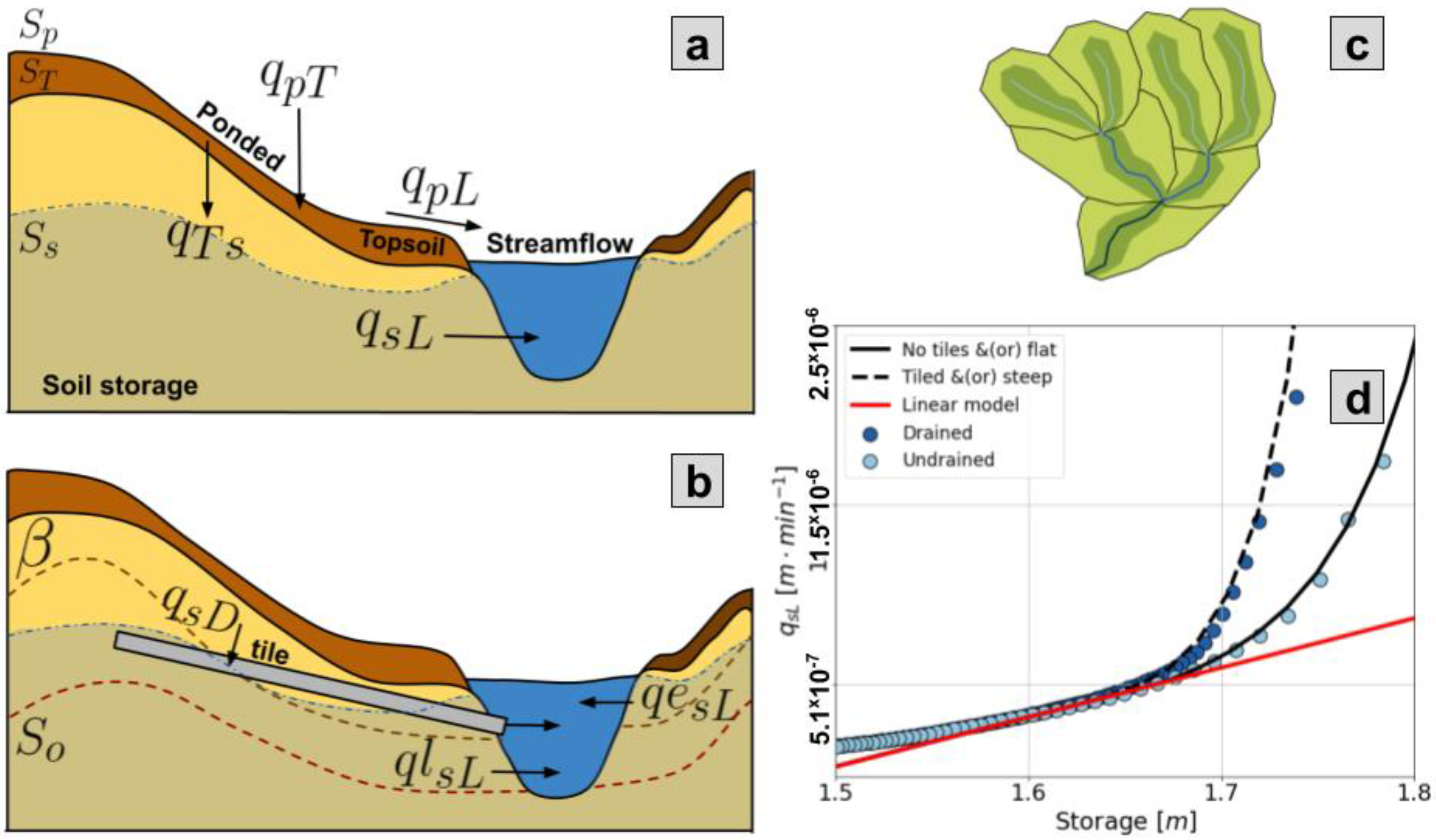
2.1. Model Description

The Hillslope Link Model (HLM) represents the hydrological processes at the hillslope scale (Figure 2a,b) and routes the streamflow through the channel network (Figure 2c). At the hillslopes, HLM has three storages, ponded surface ($S_p \left[\mathrm{m}\right])$, topsoil ($S_T \left[\mathrm{m}\right]$), and subsurface storage ($S_s \left[\mathrm{m}\right]$). The water from the ponded storage can either infiltrate the topsoil ($q_{pT }\left[\mathrm{m}\cdot {\min }^{-1}\right]$) or flow as runoff to the channel link ($q_{pL }\left[\mathrm{m}\cdot {\min }^{-1}\right]$). The water in the topsoil percolates ($q_{Ts }\left[\mathrm{m}\cdot {\min }^{-1}\right]$) to the soil storage. Finally, the water in the soil storage seeps into the channel link as subsurface runoff ($q_{sL }\left[\mathrm{m}\cdot {\min }^{-1}\right]$). Evaporation occurs from the three storages as a removal of volume from the model. Once in the river network, HLM transports the channel water ($q \left[{\mathrm{m}}^3\cdot {\mathrm{s}}^{-1}\right]$) downstream. A detailed description of the hillslope and stream routing process can be found in [11,14].

The surface runoff, infiltration, and percolation rates are linked through the reference speed $v_r$ and the shape of the hillslope. Each hillslope has a parameter $k_2\left[{\min }^{-1}\right]$ (Equation (1)) that depends on the hillslope link length ($L_i\left[\mathrm{m}\right]$) and area ($A_h\left[{\mathrm{m}}^2\right]$), along with the reference velocity $v_r$. The parameter $k_2$ is the inverse of the runoff residence time in the hillslope. The runoff $q_{pL}$ and the infiltration $q_{pT}$ are linked to $k_2$ through Equations (2) and (3), respectively. Moreover, the infiltration also depends on the topsoil depth ($T_l$) assumed to be equal to $0.1\left[\mathrm{m}\right]$. Additionally, the percolation rate $q_{Ts}$ is computed as a proportion of $k_2$, expressed by $k_i$. Usually, $k_i$ is 2% of $k_2$; however, its value may change depending on the soil and topographical properties.

$$k_2=v_r\cdot \left(\frac{L_i}{A_h}\right)\cdot 60$$

(1)

$$q_{pL}=k_2\cdot S_p$$

(2)

$$q_{pT}=k_2\cdot S_p\cdot 99\cdot {\left(1-S_T/T_l\right)}^3$$

(3)

$$q_{Ts}=k_2\cdot S_T\cdot k_i$$

(4)

The current HLM setup represents the subsurface flux to the channels ($q_{sL}\left[\mathrm{m}\cdot {\min }^{-1}\right]$) with a linear equation (red line on Figure 2d). The equation releases water to the channel at a rate $m$, when $S_s$ is greater than the no-flow threshold ($S_o$), as follows,

$$q_{sL}=m\cdot \left(S_s-S_o\right)$$

(5)

Ref. [17] developed a set of parameterizations for ordinary differential equations that adds a non-linear component to Equation (5) when $S_s$ is above threshold storage. The following exponential equation (continuous line on Figure 2d) is added to Equation (5) if $S_s$ is greater than the activation threshold $\beta \left[\mathrm{m}\right]$,

$$q{e}_{sL}=\alpha \left(S_s-\beta \right)e^{17\left(S_s-\beta \right)}$$

(6)

where $\alpha$ is a parameter that depends on the hillslope properties, such as its steepness and the soil conductivity. In [17], the authors also developed an exponential equation that applies when the hillslope has tiles. The following equation (dashed line on Figure 2d) is added when $S_s$ is greater than the tile relative depth $D_d\left[\mathrm{m}\right]$,

$$q_{sD}=c\left(S_s-D_d\right)e^{35\left(S_s-D_d\right)}$$

(7)

In the described scheme, the subsurface flux becomes a set of equations that HLM activates, depending on the value of $S_s$ relative to the thresholds $S_o$, $\beta$, and $D_d$. The segmented subsurface runoff is as follows,

$$q_{s}L=\{\begin{array}{ccc}q{l}_{sL}& if& S_s<\beta \\ q{l}_{sL}+q{e}_{sL}& if& S_s>\beta \\ q{l}_{sL}+q{e}_{sL}+q_{s}D& if& S_s>D_d\end{array}$$

(8)

The relative tile depth ($D_d$) is independent of $\beta$, so either could be larger depending on the tile configuration and the hillslope properties. Moreover, if there are no tiles, Equation (8) is limited to its two first expressions. More details on the subsurface equation development can be found in [17].

2.2. Model Setup and Data

We used both diagnostic and prognostic approaches to test the performance using the non-linear equation. We used the river network for the state of Iowa derived from a DEM of 90 m and decomposed into about 420,000 individual hillslopes, following the approach presented in [11]. The precipitation force corresponds to hourly Stage IV QPEs [24]. We forced the evapotranspiration using the mean annual monthly values derived from MODIS [25] for the region.

Equation (8) offers a formulation for the subsurface flux that we want to validate for the Iowa domain. In this process, we can fix parameters uniformly over the space or distribute them spatially. A uniform setup assumes that each hillslope in the region uses the same model parameters, while a distributed setup assumes parameter variability as a function of landscape properties. Neither approach is without error because the parameters are only approximate and could depend upon unknown factors that are variable in space. The fixed setup is unrealistic, and the distributed setup may be subject to spatial errors. However, both approaches are complementary. Fixed setups could help assess the ability of Equation (8) to improve the accuracy of the simulated streamflow fluctuations. In contrast, a distributed setup helps to validate the parameter description given by the map(s). Considering this, we used both approaches to validate the new $q_{sL}$ equation and to explore the limits of the so-called predefined setups. In the distribute parameters case, we use the steepness of the hillslopes (Figure 3a) and the tiles localization according to the Iowa Department of Natural Resources (DNR) (Figure 3b).

The model validation consists of comparing fixed (diagnostic) and distributed (prognostic) HLM setups (Figure 4). The diagnostic setup (Figure 4a) shows how different formulations could significantly improve the model across the region. On the other hand, the prognostic setups (Figure 4b) show the improvements and limitations derived from the application of “known” spatial variables.

The formulation of Equation (8) relies on the percolation rate because the non-linear formulation depends upon the amount of water in the subsurface storage. The described dependence increases the relevance of the percolation parameter ($k_i$). The distribution of $k_i$ can be derived from maps of the soil profile properties. However, using an additional map may increase the errors affecting the comparison of both setups. For this reason, we choose to fix three different percolation rates for the diagnostic and prognostic setups (Figure 4c).

Moreover, we used the same values for $S_0$, $\beta$, and $D_d$ in both setups. In [17] $S_0$ oscillates between 1.4 and 1.55 in function of the slope. Nevertheless, additional features of the hillslope such as the bedrock depth, and soil type determine the value of $S_0$. To avoid adding additional uncertainty sources, we fixed $S_0=1.48$. On the other hand, for $\mathsf{\beta }$ and $D_d$ we used the values described by [17] of 1.67 and 1.635, respectively. In

Table 1. HLM diagnostic and prognostic setups summary.

Identifier	Type	Slope	Tiled	${\mathit{k}}_{\mathit{i}}$
D1	Diagnostic	0%	False	0.02
D2	Diagnostic	2%	False	0.02
D3	Diagnostic	5%	False	0.02
D4	Diagnostic	2%	True	0.02
D5	Diagnostic	0%	False	0.03
D6	Diagnostic	2%	False	0.03
D7	Diagnostic	5%	False	0.03
D8	Diagnostic	2%	True	0.03
D9	Diagnostic	0%	False	0.04
D10	Diagnostic	2%	False	0.04
D11	Diagnostic	5%	False	0.04
D12	Diagnostic	2%	True	0.04
P1	Prognostic	Variable	Variable	0.02
P2	Prognostic	Variable	Variable	0.03
P3	Prognostic	Variable	Variable	0.04

we summarize the described diagnostic and prognostic setups.

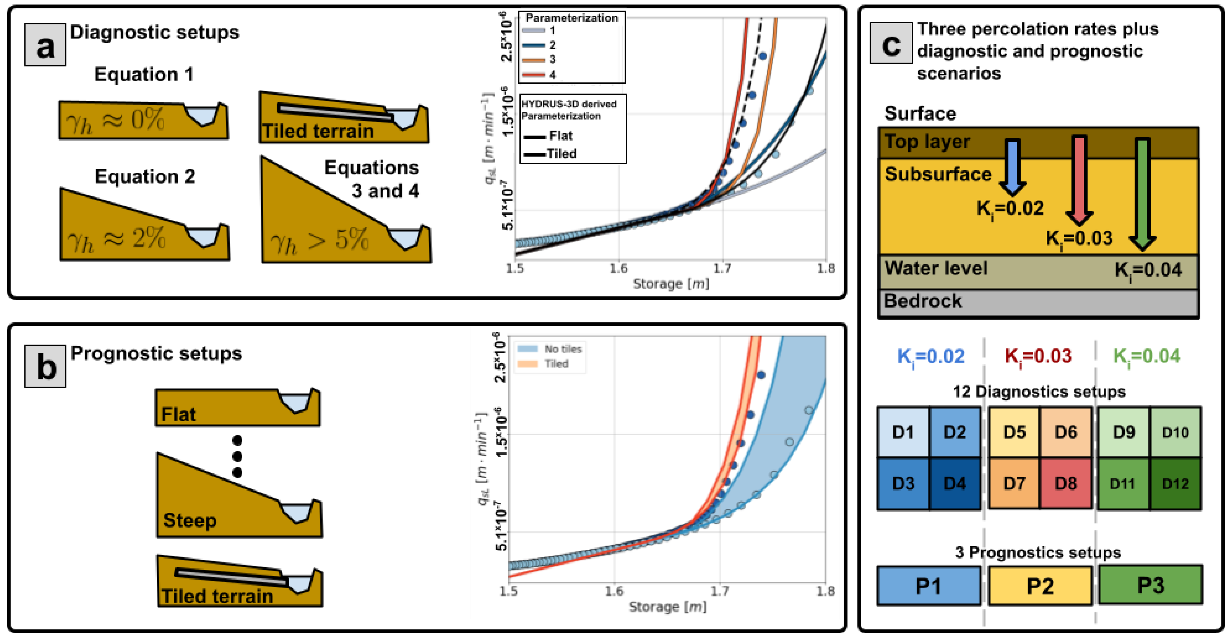
2.2.1. Diagnostic Setups

In the diagnostic setup (Figure 4a), we created four base parametrizations, using Equation (8) for the Iowa domain. The parametrizations range from flat hillslopes (light blue line on Figure 4a) to steep or tiled hillslopes (red line on Figure 4a). In the tiled case, we used a steepness of 2% under the assumption that tiles are usually installed in flat terrains. Then, we combined the four parameterizations and the three $k_i$ rates to obtain 12 diagnostic (D) scenarios (D1 to D12 in Figure 4c). In the scenarios, D1 to D4 use $k_i=0.02$; D5 to D8 use $k_i=0.03$; and D9 to D12 use $k_i=0.04$. A summary of the diagnostic scenarios is provided in Table 1.

2.2.2. Prognostic Setups

In the prognostic setup, we distributed parameter values in function of the hillslopes steepness and the Iowa DNR map describing tile presence (Figure 4b). According to [17] the coefficient $\alpha$ of Equation (6) changes in function of the hillslope steepness (${\gamma }_h$) with a linear equation. Using the following equation, we assigned the parameter $\alpha$ to each hillslope, obtaining variable $q_{s}L$ curves that oscillate between the blue bands shown in Figure 4b:

$$\alpha ={\gamma }_h\left(8.5\ast {10}^{-8}\right)+9.48\ast {10}^{-7}$$

(9)

Additionally, we include Equation (8) for tiled terrain. To do it, we assigned tiles to the hillslopes based in the map in Figure 4b. In the tile drainage case, we changed c in function of the slope using the following equation:

$$c=3.4\ast {10}^{-8}\cdot log\left({\mathsf{\gamma }}_h\right)+5.7\ast {10}^{-7}$$

(10)

Then, we developed the prognostic (P) scenarios P1, P2, and P3 using the distributed parameters $\alpha$ and $c$ with the percolation rates $k_i$ of 0.02, 0.03 and 0.04, respectively (distributed setups in Figure 4c). A summary of the prognostic scenarios is provided in Table 1.

3. Results

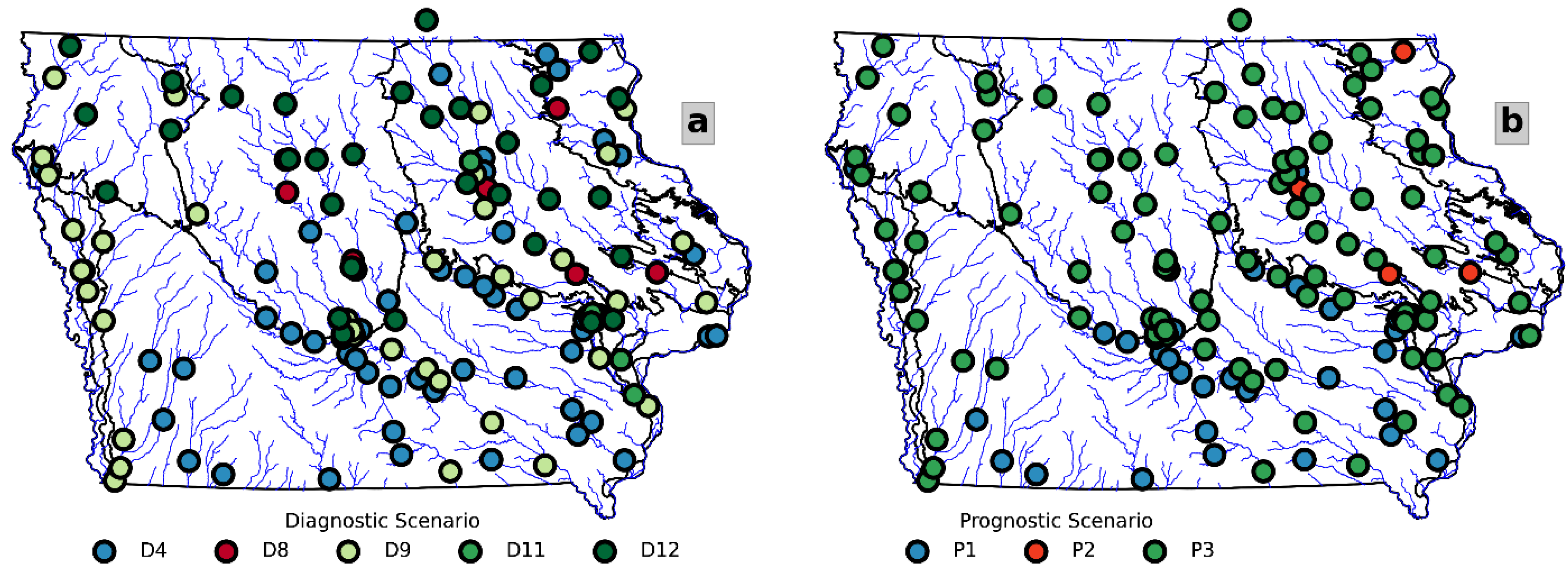
3.1. Insights from a Diagnostic-Prognostic Approach

The diagnostic and prognostic setups produced significant differences between the model outputs. In Figure 5, we present the simulated hydrographs at three watersheds simulated by the diagnostic scenario D4 in blue and the prognostic scenario P1 in red. In this case, the diagnostic setup assumes that all the hillslopes have tiles or are steep. On the other hand, the prognostic setup assumes there to be tiles only at some hillslopes and that the parameter $\alpha$ of Equation (6) varies with the steepness. In these three cases, the diagnostic (or fixed) setup produces a longer recession curve than the one obtained by the prognostic setup. The diagnostic case has a better match to the Iowa River at Tama (Figure 5b), while the prognostic setup exhibits a better match to the White Breast Creek (Figure 5a) and at the Cedar River (Figure 5c). Figure 5 gives a brief description of the expected differences between the setups. Additionally, it shows that Equation (8) can improve the streamflow representation, given the correct set of parameters that are obtained.

According to Figure 5, the non-linear model can produce a good representation of the hydrograph falling limb and early recession, depending on the parameters. Considering the described sensitivity, we compare the event-based KGE of the non-linear setups and the linear model (Figure 6). The KGE equation summarizes the correlation ($\gamma$), the mean ratio ($\mu$), and the deviation ratio ($\sigma$). Our results suggest that the KGE performance depends heavily on the percolation rate ($k_i$). With $k_i=0.02$ (first row of Figure 6), all the non-linear setups tend to improve the linear model, with a significant performance decrease in some events. Conversely, values of $k_i$ equal to 0.03 and 0.04 do not exhibit a significant KGE change (second and third rows of Figure 6). Cases such as D5 and D11 exhibited a performance such as that obtained by the linear model. Other cases, such as D9, tended toward a general decrease in performance. D6, D8, and P2 exhibited a slight performance increase. The described results highlight the relevance of the percolation rate and the subsurface parameters. The comparison with the linear model shows that Equation (8) can significantly improve the model performance, depending on the parameters.

Differences among the scenarios are highlighted by comparing the performance gauge by gauge. First, we choose the diagnostic (D) and prognostic (P) setup with the best performance at each gauge. For this, we used the KGE to select the setup that outperformed the others for most of the events. In Figure 7, we present the KGE distribution and the percentage of time each scenario was chosen. We found similarities between the diagnostic and prognostic chosen setups when grouped by the percolation rate values ($k_i$). D4 and P1 ($k_i=0.02$) have a similar KGE distribution, as do D8 and P2 ($k_i=0.03$) and the group that includes D9, D11, D12, and P3 ($k_i=0.04$). The similarities among the described groups highlights the relevance of $k_i$. Moreover, some differences also highlight the relevance of Equation (8) parameters.

The results presented in Figure 7 follow a spatial distribution. Figure 8 shows each USGS gauge colored by the diagnostic (Figure 8a) and prognostic (Figure 8b) setups with the best performance. In both cases, the percolation rate defines the spatial distribution. We can identify how the chosen setups (Figure 8) follow the Iowa landforms to some extent in the diagnostic case (see Figure 3a). Scenario D12 is recurrent over the Des Moines Lobe and the Northwest Iowa Plain. D9 recurs over the Missouri River Alluvial and Loess Hills landforms. We found that D4 dominates over the Southern Iowa Drift area. In the remaining regions, we see a mix of scenarios. The spatial distribution is similar among the chosen prognostic scenarios (Figure 8b) and seems to be highly influenced by the percolation rates, represented here by tones of blue ($k_i=0.02)$, red ($k_i=0.03)$, and green ($k_i=0.04)$.

According to Figure 8, the chosen diagnostic and prognostic scenarios share percolation rates. However, differences exist in the spatial performance improvement distribution (Figure 9). Figure 9a,b show the diagnostic and prognostic scenarios of KGE improvement with respect to the linear model. With only two cases of negative KGE differences (red dots on Figure 9a), the diagnostic scenarios outperform the linear model at almost all the USGS gauges. Alternatively, in the prognostic case (Figure 9b), the count of negative KGE differences increases to 13, while the number of gauges decreases in cases where the improvement is more significant than 0.1 (yellow). We attribute the decrease in prognostic case performance to the parameter’s spatial distribution.

The prognostic scenario performance decrease occurs mostly over the east and west regions of Iowa. The most significant decrease is observed for the Northwest Iowa Plains landform (Figure 9b). In this region, the chosen diagnostic setups were D12 and D9 (Figure 8a), suggesting a mix between tiled terrain and flat hillslopes. Over the Southern Iowan Drift landform area, the $k_i$ value is the same for the diagnostic and prognostic scenarios. However, the prognostic scenario performance declines at several stations in this region. On the other hand, the Iowa Surface region exhibits more $k_i$ discrepancies between both scenarios, as well as a higher number of performance differences.

The described results suggest a level of heterogeneity in the parameters shown by the diagnostic and prognostic scenarios. This heterogeneity creates difficulties when choosing the most adequate regional parameterization for the model, regardless of whether it is fixed (diagnostic) or distributed (prognostic). To address this issue, we compare the KGE (upper diagonal in Figure 10) and the mean ratio $\mu$ (lower diagonal in Figure 10) of the chosen scenarios. We estimate $\mu$ as the ratio between the simulated (${\mu }_{sim}$) and observed (${\mu }_{obs}$) flows with values near indicating a perfect match. According to Figure 10, the KGE and mean ratio of scenarios D4 and P1 outperform almost all the scenarios. Additionally, both scenarios have the highest percentage of events with KGE values above 0.4 (blue bars in Figure 10 histograms). Compared with the linear model, the D4 and P1 mean ratio correction is significant. In both plots (Linear-D4 and Linear-P1), there are almost no events where the linear setup outperformed D4 and P1. The scenarios D4 and P1 have the same $k_i$ (0.02) value; however, their subsurface parameters are different.

The parameters of D4 are fixed for all the domains following line 4 of Figure 4a. This parameterization represents highly conductive soils or the presence of tiles. On the other hand, P1 parameters follow the hillslope steepness with Equation (9), and the presence of tiles described by the map in Figure 4b. The described differences in the parameters seem to develop slight dissimilarities in performance. According to panel D4-P1 in Figure 10, the KGE performance is similar in both, although D4 has a better performance in some events. Moreover, the panel P1-D4 shows that the mean ratio description of both setups is similar. Considering that D4 assumes tiles everywhere, our results suggest a high presence of tile-like signatures.

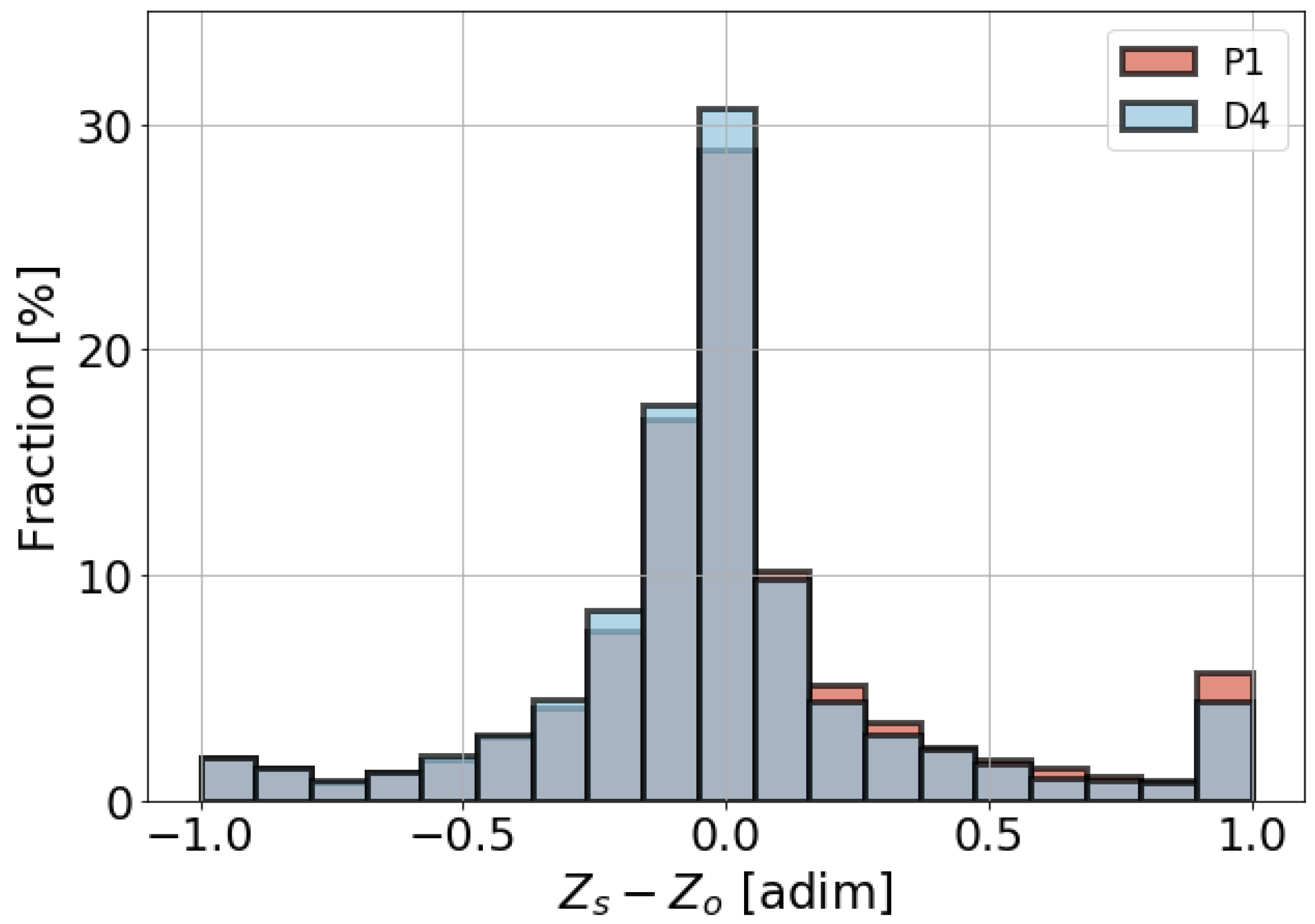
3.2. Extended Metrics

According to the diagnostic and prognostic KGE comparisons, the performance differences between the two scenarios are relatively small. However, the KGE is subject to three parameters that do not necessarily reflect all the relevant changes in the simulated streamflows. With this in mind, we also compared the NSE (Nash Sutcliffe efficiency), the hit rate, and the lags (Figure 11a–c, respectively). The NSE contrasts the simulated data prediction skill with the mean value of the observations. An NSE of below 0 indicates that the mean value performs better than the model, and an NSE of 1 indicates a perfect simulation. The hits rate is the percentage of time that is shared by observations and simulations during floods. A hit rate of zero corresponds to missing all the floods, and a hit rate of one corresponds to a perfect match. The lag is a measure of the displacements applied over the simulated data to maximize the correlation. We made hourly displacements from −48 h to 48 h. Negative lag values correspond to cases in which the simulated data exhibit responses earlier than the observed, and positive values correspond to the opposite behavior. A simulated series with good performance must have lags near zero.

Results from Figure 11 show that D4 and P1 have some similarities and some relevant differences. Regarding the NSE (Figure 11a), D4 has a slightly better score. Regarding the hits rate (Figure 11b), it is hard to tell which scenario has a better performance. Furthermore, P1 has a higher fraction of hit rates approaching one, but it also has higher frequencies at some lower intervals. The number of lags is also similar (Figure 11c). Nevertheless, P1 tends toward negative lag values more than D4 does, representing more frequent early peak estimations.

In addition to the indexes, we compare the simulated peaks of the chosen diagnostic and prognostic scenarios. Because the gauged watersheds areas range between 40 and 18,000 ${\mathrm{km}}^2$, we performed a scale-independent comparison. To obtain scale-independent peaks ($Z$), we divided the peaks $Q_p \left[{\mathrm{m}}^3\cdot {\mathrm{s}}^{-1}\right]$ by the mean annual peak $\overline{Q_p} \left[{\mathrm{m}}^3\cdot {\mathrm{s}}^{-1}\right]$. Then, for each event of each link, we computed the difference between the simulated ($Z_s$) and the observed ($Z_o$) standardized peaks. The peak flow estimation of D4 and P1 exhibited a similar performance, with D4 being superior. The D4 scenario reaches a fraction of 32% for differences near zero (Figure 12), while in P1 this value drops to 28% (Figure 12). Additionally, P1 has a higher fraction of errors equal or greater than one.

We expected the diagnostic superiority because, in the prognostic case, we impose restrictions based on maps. The resulting differences among simulations emphasize the parameters’ relevance and the need for their correct representation. Contrasted with the diagnostic scenarios, the prognostic scenarios tend to reduce the performance. The differences between D4 and P1 suggest that the landscape descriptors could have errors that lead to decreases in the modeling performance. Additionally, our results suggest that there may be more tiles than the ones represented by the map in Figure 4b.

3.3. Analysis of Parameter Values

The diagnostic and prognostic scenarios offer different ways to determine the values of parameters in space. In the diagnostic cases, we identified the best fixed-parameter combination for each gauged watershed. In the prognostic cases, we pre-defined a set of distributed parameters based on the available information. In a previous step, we defined the best diagnostic and prognostic setup for each gauge (Figure 8a,b, respectively). According to our results, a spatial distribution of the parameters seems to be explained by $k_i$ and the parameters of Equation (8). Additionally, the chosen diagnostic scenarios outperform the chosen prognostic ones (Figure 8a,b). In some gauges, the performance differences are small; however, in others, the difference is relatively large. This is an interesting result because the only difference between both cases is the parameterization of Equation (8). Considering the described performance differences, we explore in more detail how they are related to the parameterizations of the diagnostic and prognostic setups.

We compare Equation (8) setup for the diagnostic and prognostic scenarios to evaluate whether variations in the parameters explain the observed performance differences. We made the comparison at each gauged watershed. For the comparison, the prognostic setup has a set of curves $q_{sL}\left(P\right)$ for a given watershed (light blue lines in Figure 13), and there is one diagnostic curve $q_{sL}\left(D\right)$ for the same watershed (dark blue line in Figure 13). Using Equation (11), we compare $q_{sL}\left(D\right)$ with the 50th percentile of $q_{sL}\left(P\right)$ for storages between 1.6 and 1.7 $\left[\mathrm{m}\right]$ (green region in Figure 13). We choose the 1.6–1.7 range because it describes the shift the linear to the exponential expression. Besides, the hillslopes subsurface storage ($S_s$) is usually in this range during storm events.

$$\mathsf{\Delta }{q}_{sL}=\frac{1}{N}\cdot {{\displaystyle \sum }}_i^N\frac{q_{sL}{\left(D\right)}_i-P50{(q_{sL}\left(P\right))}_i}{q_{sL}{\left(D\right)}_i}$$

(11)

According to Figure 14, the differences of the parameters ($\mathsf{\Delta }{q}_{sL}$) do not adequately explain the performance differences between the diagnostic and the prognostic scenarios. In some cases, low absolute values of $\mathsf{\Delta }{q}_{sL}$ are linked to low KGE differences. However, the described behavior does not apply for large absolute values of $\mathsf{\Delta }{q}_{sL}$. Figure 14 shows many watersheds in which the differences of the absolute parameters are larger than 10% (x-axis), while the KGE absolute differences are low. Additionally, some cases with low absolute $\mathsf{\Delta }{q}_{sL}$ exhibit large KGE differences. On the other hand, according to the colors of Figure 14 (non-absolute $\mathsf{\Delta }{q}_{sL}$), positive values of $\mathsf{\Delta }{q}_{sL}$ are related to low KGE differences; and negative values of $\mathsf{\Delta }{q}_{sL}$ correspond to high KGE differences.

We also compared the $\mathsf{\Delta }{q}_{sL}$ and the KGE differences in space. According to Figure 15, the coincidences between the KGE and $\mathsf{\Delta }{q}_{sL}$ do not show a strong regional pattern. We observe some similarities only in the Des Moines Lobe and the Northwest Iowa Plains regions. In both cases, some significant KGE differences correspond with large absolute $\mathsf{\Delta }{q}_{sL}$ values. Additionally, there is a match between low KGE and $\mathsf{\Delta }{q}_{sL}$ differences in the Iowan Surface region, with some exceptions.

It is hard to establish a relationship between the diagnostic and prognostic parameters and their performance differences. We attribute this lack of correlation to the model’s non-linear transformations at the hillslope scale and throughout the network. It is expected that the parameters would alter the model’s output. However, our results show that a pre-defined distribution of the parameters could lead to modeling errors that are hard to identify.

4. Conclusions

The Iowa Flood Center (IFC) has been making operational flood forecasts for the state of Iowa since 2010. IFC forecasters use the hydrological Hillslope Link Model (HLM), along with rainfall data. The HLM has been accurate in forecasting streamflow fluctuations at several scales [14]. However, the model has limitations in its representation of the recession curve, and it underestimates the total streamflow volume. Moreover, the limitations seem to increase in a tiled landscape. The authors of [17] attributed these limitations to the linear equation HLM uses to represent the subsurface flux and the lack of an equation representing the tiled terrain. To address this issue, [15] developed an exponential equation that can be parameterized to represent the function of the hillslope steepness and the presence of tiles.

This paper evaluated the exponential equation proposed by [17], which represents subsurface hillslope–link interaction in HLM. The equation can represent hillslopes with and without tile drainage. We performed the equation evaluation at 140 USGS gauges in Iowa. The analysis used hourly records between 2002 and 2018. In the evaluation, we compared the exponential equation with a linear equation. The comparison used a diagnostic and a prognostic approach to establish the parameters. In the diagnostic setup, we implemented 12 fixed parameter scenarios, while in the prognostic setup, we distributed the parameters with consideration of the hillslope steepness and presence of tiles. In both cases, we considered three fixed percolation rates. Results from this study indicate the following:

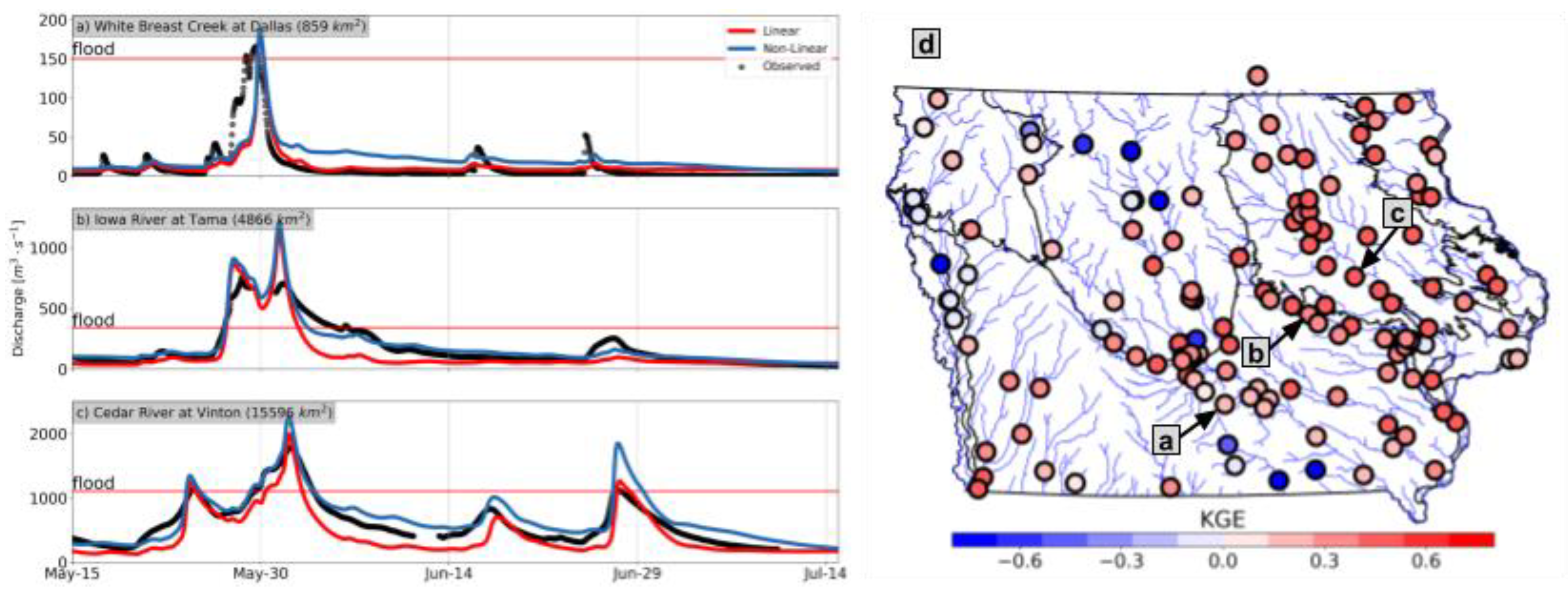
• Compared with the linear equation, the exponential equation corrects the volume bias on the simulated streamflow. We attribute the correction to the active layer threshold on the exponential equation and the significant outflow increase once the storage is above this threshold. In contrast, in the linear equation, the water remains in the soil for extended periods because of the described absence of these processes.
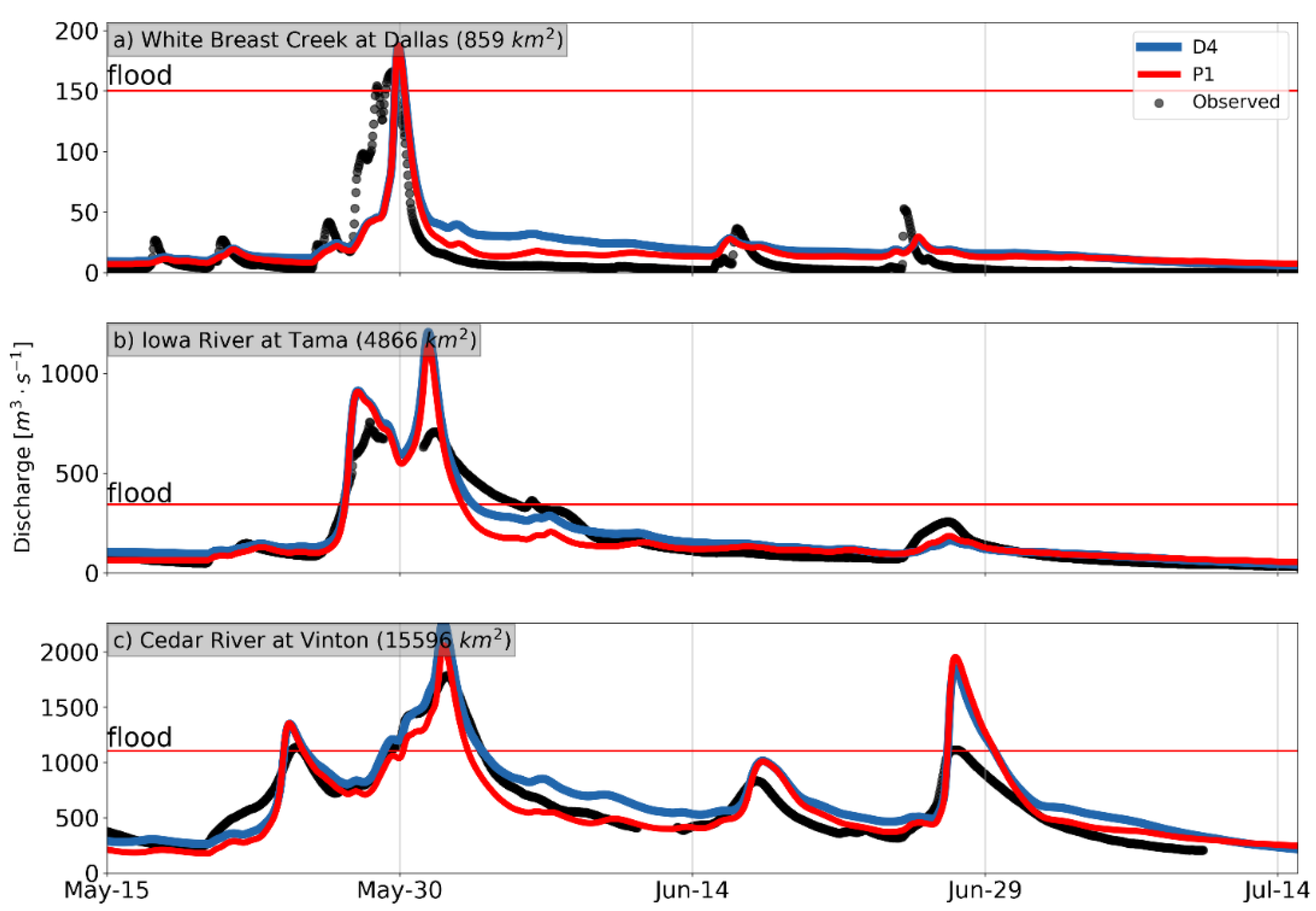
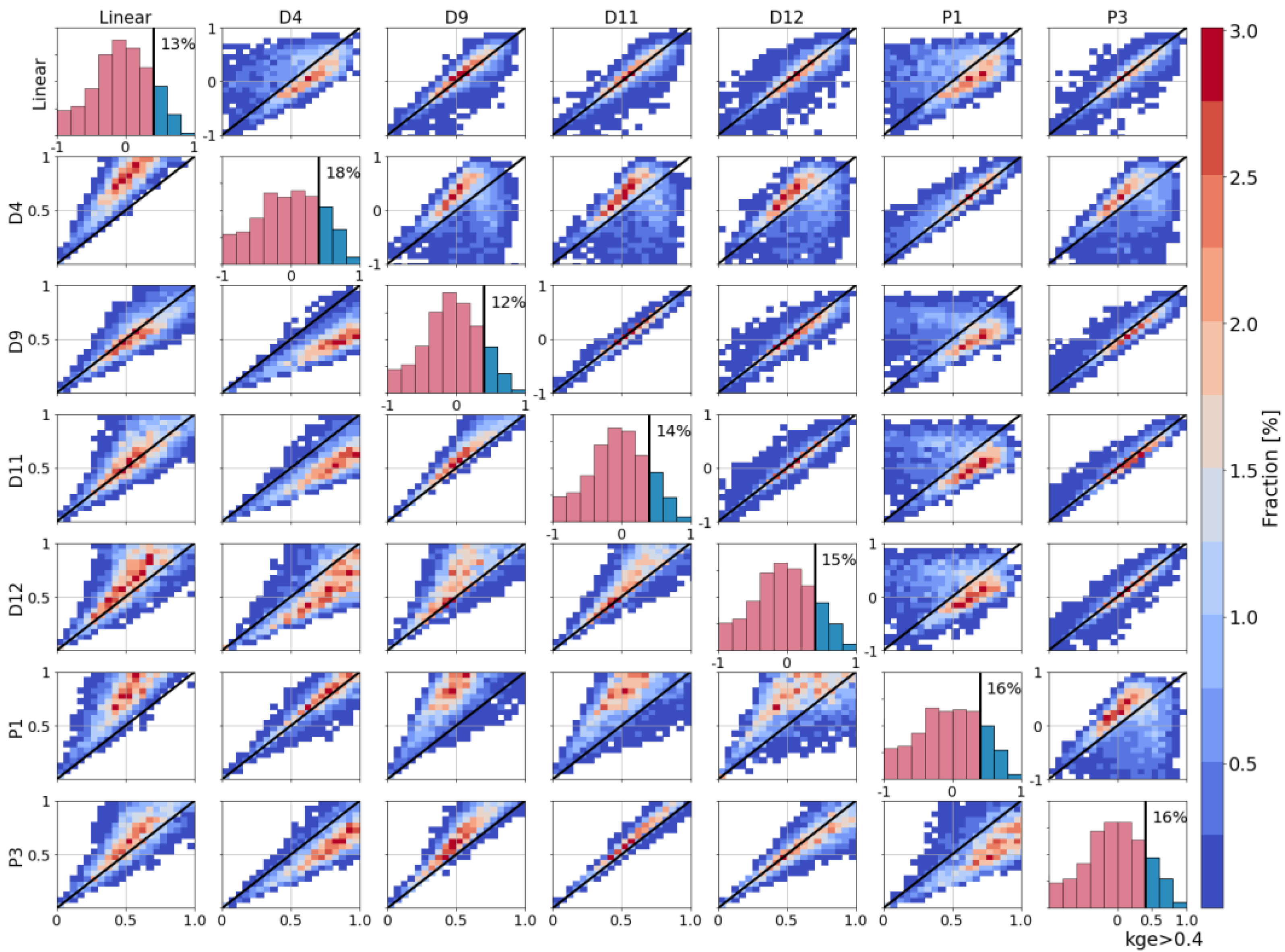
• Depending on the parameters, the exponential equation could improve the performance of HLM. We found that the exponential equation outperforms the linear equation for several parameter combinations with changes in the shape of the hydrograph, the simulated peaks, and timing. We also found significant differences using different combinations of the equation parameters and the percolation rate.
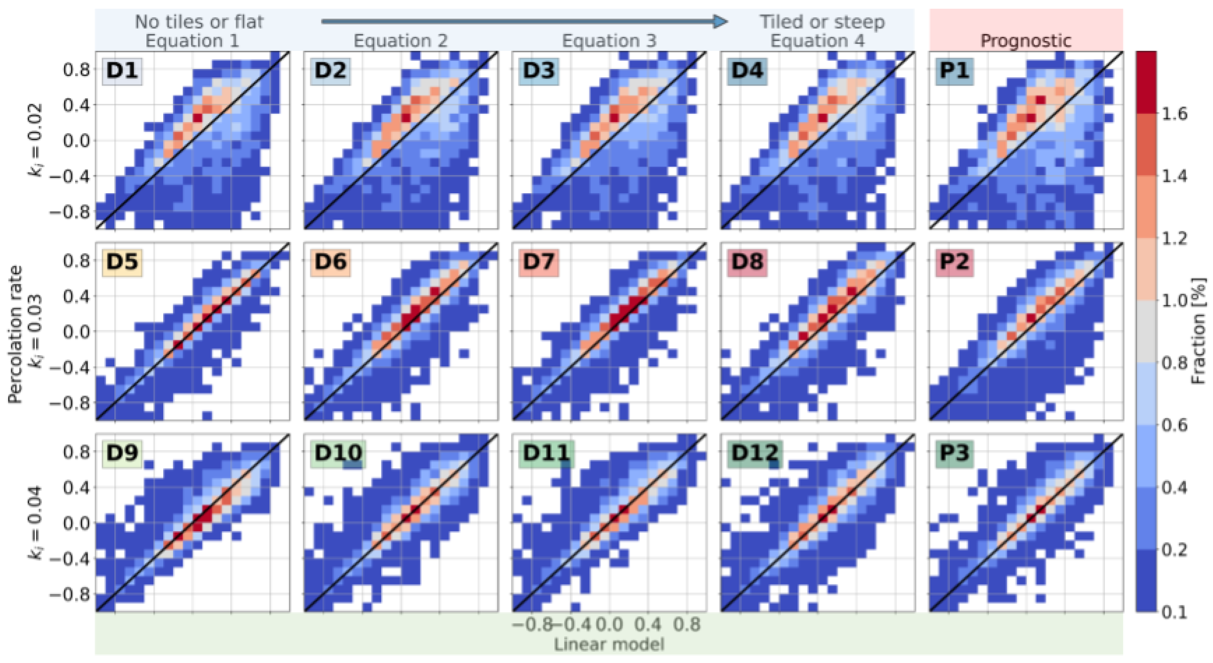
• The percolation rate plays a significant role in the representation of the subsurface flux from the described combinations. We found spatial coincidences in the percolation rates when choosing the best diagnostic and prognostic scenarios. Additionally, the percolation rate induces changes comparable to those produced by the exponential equation’s parameters.
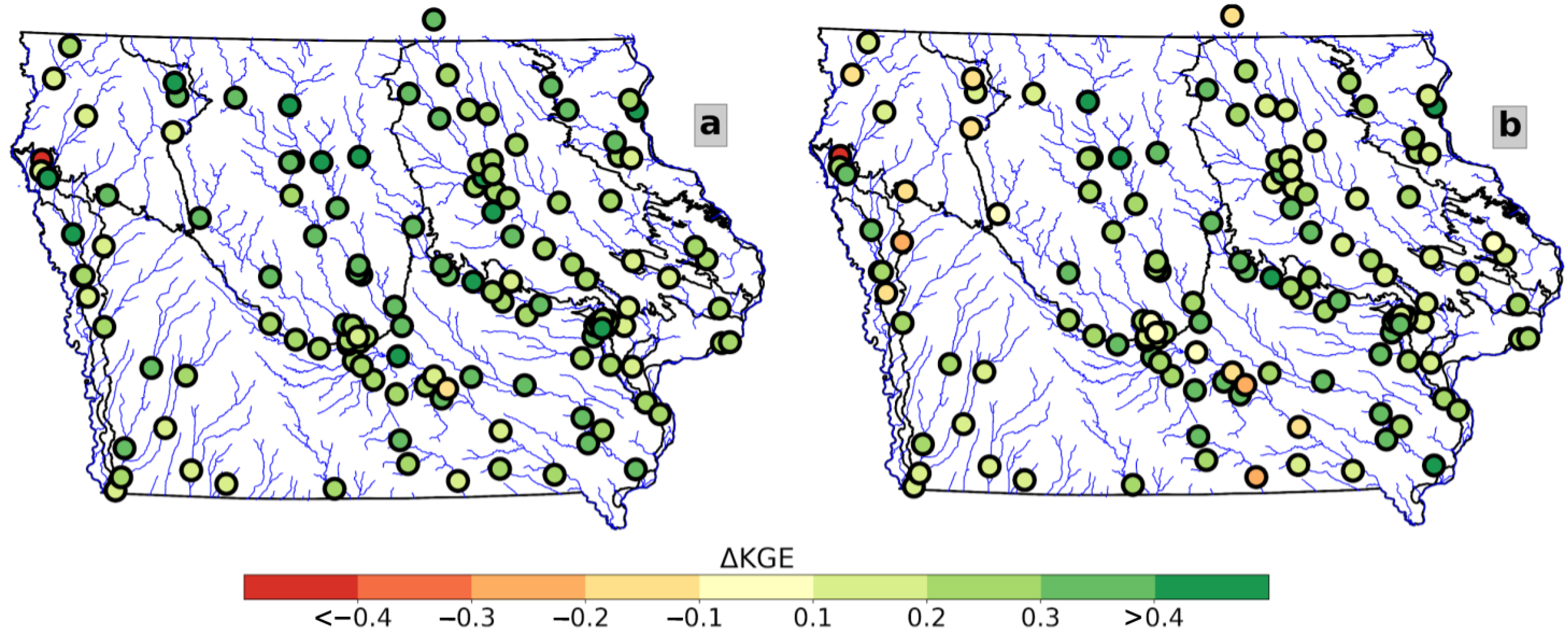
• Determining the distributed parameters of HLM remains challenging. In this paper, we used the diagnostic and prognostic approaches to analyze the parameters of HLM. The diagnostic approach assumes unknown conditions and fixed parameters over the space. On the other hand, the prognostic method is the more classical approach, in which the parameters are derived from maps of the landscape. In our experiments, the diagnostic setups tended to outperform the prognostic setups. Additionally, had difficulty in identifying a link between the diagnostic and prognostic parameters and their respective performances.

In the current work, we showed that a better representation of the processes and the correct parameters can improve a hydrological model. The improvement is supported by comparisons performed at 140 USGS gauges. Moreover, the differences between the diagnostic and prognostic setups suggest that identifying the parameters is still challenging. Despite the limitation related to the number of gauges, the diagnostic approach reveals the parameters’ potential spatial distribution.

Two main factors may explain the differences in parameters and performance between the diagnostic and prognostic setups: errors in the landscape description and unrepresented processes in HLM. Uncertainties exist in the tile localization maps; likewise, limitations exist in the representation of the average steepness at the hillslope scale. On the other hand, we unrepresented processes in some regions of Iowa, such as potholes over the northwest and agricultural terraces in the west. It is difficult to identify which of these factors is more relevant to the implementation of a hydrological model. However, according to our results, the use of maps as landscape descriptors may lead to the detection of errors that are usually hidden in a posterior calibration process. Moreover, we found it difficult to identify the errors caused by the prescribed distributed parameters. Both issues could be addressed using diagnostic setups that help to identify the uncertainties derived from the parameters and their possible regional distributions.

References

1. Samaniego, L.; Kumar, R.; Attinger, S. Multiscale parameter regionalization of a grid-based hydrologic model at the mesoscale. Water Resour. Res. 2010, 46, 1–25. [Google Scholar] [CrossRef] [Green Version]
2. Mandeville, A.N. Insights gained from four component hydrograph separation. Hydrol. Res. 2016, 47, 606–618. [Google Scholar] [CrossRef]
3. Chen, B.; Krajewski, W.F. Recession analysis across scales: The impact of both random and nonrandom spatial variability on aggregated hydrologic response. J. Hydrol. 2015, 523, 97–106. [Google Scholar] [CrossRef]
4. Clark, M.P.; Rupp, D.E.; Woods, R.A.; Tromp-van Meerveld, H.J.; Peters, N.E.; Freer, J.E. Consistency between hydrological models and field observations: Linking processes at the hillslope scale to hydrological responses at the watershed scale. Hydrol. Process. 2009, 23, 311–319. [Google Scholar] [CrossRef]
5. Harman, C.J.; Sivapalan, M.; Kumar, P. Power law catchment-scale recessions arising from heterogeneous linear small-scale dynamics. Water Resour. Res. 2009, 45, 1–13. [Google Scholar] [CrossRef] [Green Version]
6. Tallaksen, L.M. A review of baseflow recession analysis. J. Hydrol. 1995, 165, 349–370. [Google Scholar] [CrossRef]
7. Biswal, B.; Marani, M. Geomorphological origin of recession curves. Geophys. Res. Lett. 2010, 37, 1–5. [Google Scholar] [CrossRef]
8. Shaw, S.B.; Riha, S.J. Examining individual recession events instead of a data cloud: Using a modified interpretation of dQ/dt-Q streamflow recession in glaciated watersheds to better inform models of low flow. J. Hydrol. 2012, 434–435, 46–54. [Google Scholar] [CrossRef]
9. Zhang, Z.; Li, Y.; Wang, X.; Li, H.; Zheng, F.; Liao, Y.; Tang, N.; Chen, G.; Yang, C. Assessment of river health based on a novel multidimensional similarity cloud model in the Lhasa River, Qinghai-Tibet Plateau. J. Hydrol. 2021, 603, 127100. [Google Scholar] [CrossRef]
10. Schilling, K.E.; Gassman, P.W.; Arenas-Amado, A.; Jones, C.S.; Arnold, J. Quantifying the contribution of tile drainage to basin-scale water yield using analytical and numerical models. Sci. Total Environ. 2019, 657, 297–309. [Google Scholar] [CrossRef] [PubMed]
11. Schilling, K.E.; Helmers, M. Effects of subsurface drainage tiles on streamflow in Iowa agricultural watersheds: Exploratory hydrograph analysis. Hydrol. Processes Int. J. 2008, 4506, 4497–4506. [Google Scholar] [CrossRef]
12. Mantilla, R.; Gupta, V.K. A GIS Numerical Framework to Study the Process Basis of Scaling Statistics in River Networks. October 2005, 2, 404–408. [Google Scholar] [CrossRef]
13. Demir, I.; Krajewski, W.F. Towards an integrated Flood Information System: Centralized data access, analysis, and visualization. Environ. Model. Softw. 2013, 50, 77–84. [Google Scholar] [CrossRef]
14. Krajewski, W.F.; Ceynar, D.; Demir, I.; Goska, R.; Kruger, A.; Langel, C.; Mantilllla, R.; Niemeier, J.; Quintero, F.; Seo, B.C.; et al. Real-time flood forecasting and information system for the state of Iowa. Bull. Am. Meteorol. Soc. 2017, 98, 539–554. [Google Scholar] [CrossRef]
15. Quintero, F.; Krajewski, W.F.; Seo, B.C.; Mantilla, R. Improvement and evaluation of the Iowa Flood Center Hillslope Link Model (HLM) by calibration-free approach. J. Hydrol. 2020, 584, 124686. [Google Scholar] [CrossRef]
16. Gupta, H.V.; Kling, H.; Yilmaz, K.K.; Martinez, G.F. Decomposition of the mean squared error and NSE performance criteria: Implications for improving hydrological modelling. J. Hydrol. 2009, 377, 80–91. [Google Scholar] [CrossRef] [Green Version]
17. Fonley, M.R.; Qiu, K.; Velásquez, N.; Haut, N.K.; Mantilla, R. Development and Evaluation of an ODE Representation of 3D Subsurface Tile Drainage Flow Using the HLM Flood Forecasting System. Water Resour. Res. 2021, 57, e2020WR028177. [Google Scholar] [CrossRef]
18. Clark, M.P.; Kavetski, D.; Fenicia, F. Pursuing the method of multiple working hypotheses for hydrological modeling. Water Resour. Res. 2011, 47, 1–16. [Google Scholar] [CrossRef] [Green Version]
19. Sur, C.; Park, S.Y.; Kim, J.S.; Lee, J.H. Prognostic and diagnostic assessment of hydrological drought using water and energy budget-based indices. J. Hydrol. 2020, 591, 125549. [Google Scholar] [CrossRef]
20. Kalma, J.D.; McVicar, T.R.; McCabe, M.F. Estimating land surface evaporation: A review of methods using remotely sensed surface temperature data. Surv. Geophys. 2008, 29, 421–469. [Google Scholar] [CrossRef]
21. Allen, R.G.; Pereira, L.S.; Howell, T.A.; Jensen, M.E. Evapotranspiration information reporting: I. Factors governing measurement accuracy. Agric. Water Manag. 2011, 98, 899–920. [Google Scholar] [CrossRef] [Green Version]
22. Yilmaz, M.T.; Anderson, M.C.; Zaitchik, B.; Hain, C.R.; Crow, W.T.; Ozdogan, M.; Chun, J.A.; Evans, J. Comparison of prognostic and diagnostic surface flux modeling approaches over the Nile River basin. Water Resour. Res. 2014, 50, 386–408. [Google Scholar] [CrossRef]
23. Crow, W.T.; Li, F.; Kustas, W.P. Intercomparison of spatially distributed models for predicting surface energy flux patterns during SMACEX. J. Hydrometeorol. 2005, 6, 941–953. [Google Scholar] [CrossRef] [Green Version]
24. Lin, Y. GCIP/EOP Surface: Precipitation NCEP/EMC 4KM Gridded Data (GRIB) Stage IV Data. UCAR/NCAR-Earth Observing Laboratory. Available online: https://data.eol.ucar.edu/dataset/21.006 (accessed on 30 November 2021).
25. Running, S.; Mu, Q.; Zhao, M. MOD16A2 MODIS/Terra Net Evapotranspiration 8-Day L4 Global 500 m SIN Grid V006. 2017. Available online: https://lpdaac.usgs.gov/products/mod16a2v006/ (accessed on 30 November 2021).
Figure 1. (ac) Observed (black) and simulated streamflows by the linear (red) and the non-linear (blue) setups at three USGS gauged stations. (d) Mean annual KGE performance of the HLM linear setup for Iowa between 2002 and 2018.
Hydrology 08 00187 g001
Figure 2. Hillslope Link Model spatial discretization and schematic of the storages and processes represented at the hillslope scale: (a) HLM hillslope process using the linear subsurface flux equation; (b) hillslope process including the active layer ( β ), the exponential flux ( q e s L ), and the tile drainage flux ( q s D ); (c) watershed decomposition into hillslopes and channel links; and (d) functional form of the subsurface flux in the function of the soil storage ( S s ) after [17].
Hydrology 08 00187 g002
Figure 3. Maps of the hillslope steepness (a) and tile drainage localization according to the Iowa DNR (b).
Hydrology 08 00187 g003
Figure 4. Diagnostic and prognostic experiment setup: (a) diagnostic case with four non-linear subsurface flux equations fixed for the domain of Iowa after [17] (b) prognostic case, with equations varying with the hillslopes steepness (blue scenario) and the presence of tiles (red scenario); and (c) percolation rates fixed for the different scenarios. Their combination gives us 12 diagnostic scenarios and three prognostic scenarios.
Hydrology 08 00187 g004
Figure 5. (ac) Diagnostic (blue) and prognostic (red) simulations done for the year 2013. Results are compared with the USGS observations (black).
Hydrology 08 00187 g005
Figure 6. Event-based KGEs comparison between the diagnostics setups and the linear model. Each row corresponds to a fixed percolation rate. Columns correspond to the four fixed equations. The color bar shows the percentage of events that fall at each bin of the 2D histogram.
Hydrology 08 00187 g006
Figure 7. Event-based KGE distribution for the selected scenarios at each station.
Hydrology 08 00187 g007
Figure 8. Spatial distribution of the scenarios with best KGE performance at each USGS station: (a) results obtained from the diagnostic scenarios; and (b) results obtained from the prognostic scenarios. The green, red, and blue gauge colors correspond to the percolation rates of 0.02, 0.03, and 0.04, respectively.
Hydrology 08 00187 g008
Figure 9. Mean KGE spatial difference of the diagnostic and prognostic scenarios with respect to the linear model: (a) diagnostic KGE minus linear model KGE; and (b) prognostic KGE minus linear model KGE.
Hydrology 08 00187 g009
Figure 10. An event-based KGE comparison of the diagnostic and prognostic dominant scenarios. Each row compares a scenario against the others. The upper diagonal panels correspond to the KGE histogram of the scenarios. Over the diagonal the KGE histogram of each setup, a coloring in of the percentage of events with blue is visible, with a KGE of above 0.4. The lower diagonal compares the event-based mean-ratio error.
Hydrology 08 00187 g010
Figure 11. Histograms of performance metrics for the scenarios D4 and P1. Panel a compares the NSE. Panel (b) compares the Hit Rate considering (a) Hit when the simulated and observed streamflow are above the flood level of the gauge. Panel (c) compares the Lags (in hours) required to maximize the correlation between observations and simulations.
Hydrology 08 00187 g011
Figure 12. Histograms of the standardized peak flows difference for the D4 (blue) and P1(red) scenarios.
Hydrology 08 00187 g012
Figure 13. Example of the q s L parameterization comparison between the diagnostic and prognostic scenarios. The light blue lines are q s L curves of the prognostic scenario for a given watershed. The red line corresponds to the 50th percentile of the prognostic q s L curves. The dark blue line is the q s L curve of the diagnostic scenario. We used the green region to perform a comparison between the scenarios.
Hydrology 08 00187 g013
Figure 14. Parameters’ absolute differences vs. KGE differences at the USGS gauges. The colors correspond to non-absolute differences in the parameters.
Hydrology 08 00187 g014
Figure 15. Maps showing KGE differences (a), and Δ q s L (b), in USGS gauges.
Hydrology 08 00187 g015