Validation of Three Daily Satellite Rainfall Products in a Humid Tropic Watershed, Brantas, Indonesia: Implications to Land Characteristics and Hydrological Modelling

Abstract

A total of three different satellite products, CHIRPS, GPM, and PERSIANN, with different spatial resolutions, were examined for their ability to estimate rainfall data at a pixel level, using 30-year-long observations from six locations. Quantitative and qualitative accuracy indicators, as well as R² and NSE from hydrological estimates, were used as the performance measures. The results show that all of the satellite estimates are unsatisfactory, giving the NRMSE ranging from 6 to 30% at a daily level, with CC only 0.21–0.36. Limited number of gauges, coarse spatial data resolution, and physical terrain complexity were found to be linked with low accuracy. Accuracy was slightly better in dry seasons or low rain rate classes. The errors increased exponentially with the increase in rain rates. CHIPRS and PERSIANN tend to slightly underestimate at lower rain rates, but do show a consistently better performance, with an NRMSE of 6–12%. CHRIPS and PERSIANN also exhibit better estimates of monthly flow data and water balance components, namely runoff, groundwater, and water yield. GPM has a better ability for rainfall event detections, especially during high rainfall events or extremes (>40 mm/day). The errors of the satellite products are generally linked to slope, wind, elevation, and evapotranspiration. Hydrologic simulations using SWAT modelling and the three satellite rainfall products show that CHIRPS slightly has the daily best performance, with R² of 0.59 and 0.62, and NSE = 0.54, and the monthly aggregated improved at a monthly level. The water balance components generated at an annual level, using three satellite products, show that CHIRPS outperformed with a ration closer to one, though with a tendency to overestimate up to 3–4× times the data generated from the rainfall gauges. The findings of this study are beneficial in supporting efforts for improving satellite rainfall products and water resource implications.

1. Introduction

Rainfall signifies an important physical variable in modulating varying ecosystem functions, including water availability [1], soil productivity [2], biodiversity, and agricultural production [3], and is of importance in supporting land and water management, such as soil erosion and flood risk assessment. Rainfall has been traditionally measured using a gauge in real-time, on a daily basis. Given the importance of rainfall data, therefore, accurate and complete rainfall data availability is essential for multi-users’ decision-making processes [4]. However, despite being considered as the most accurate rainfall data, the rainfall data are only available to the corresponding point or location of the gauges [5]. In tropical developing countries, rainfall gauges’ measurement records are often limited by lower spatial and temporal coverage, due to costly maintenance, infrastructure and difficult terrain conditions, especially in mountainous regions where an orographic influence is evident.

To provide rainfall information for ungauged places, estimation has commonly been implemented through varying techniques of interpolation, including gauge points such as arithmetic mean, Thiessen polygon, isohyet, and geo-statistics [6,7,8]. However, these methods require extensive gauge coverage and representative gauge distribution. When these factors are compromised, high bias or errors are often the consequence. The increasingly operational satellite data have offered gridded rainfall estimates in varying scales. The products offer a promising approach to providing rainfall data that support varying applications, such as drought monitoring, flood risk assessments and water balance studies [9]. However, despite their potential to provide complete rainfall data coverage, satellite-based rainfall estimates introduce a degree of error. Information about the errors of rainfall estimates is of importance in that it enables the users to identify the most suitable rainfall estimates and incorporate the errors in sequential analysis [10]. This is even more critical for hydrological applications, since the rainfall variability has often been quantified as the primary source of errors [11,12,13].

Despite improved development of satellite-based rainfall data, which has made data more reliable and accurate [14,15], a number of studies on error assessments of satellite-based rainfall data reveal that errors may vary from one region to another [10,16]. Several studies also demonstrated the inconsistency of the performance of satellite-derived rainfall data. For example, the Climate Prediction Center Morphing Method (CMORPH) data are better than Precipitation Estimation from Remotely Sensed Information using Artificial Neural Network (PERSIANN) in tropical landscapes in Bali and the Ethiopian highlands [17,18], but it showed larger bias in Sumatra [19]. As modeling products, rainfall estimates from satellite data introduce inherent errors and uncertainties due to several aspects, such as methods in spatial and temporal samplings, estimation methods of data, and climatic and terrain conditions [20,21]. Besides, satellite rainfall errors have also been found to have an association with externalities, such as geographic, topographic, and climatic regimes [22,23,24]. This condition drives the need for a comprehensive validation assessment in varying geographic areas to improve the usability of remote sensing-based rainfall products.

Indonesia is a typical tropical country with distinct monsoonal characteristics in most parts. The presence of extensive mountainous regions signifies the role of orographic influences. As in other humid tropic regions, primary traits include intensified rainfall energy, leading to a great amount of runoff, and subjectivity to massive land-surface disturbance [25]. When national and local rain gauges’ data coverage is inaccessible, incomplete, and insufficient, a reliance on satellite rainfall data is an increasingly used alternative for varying assessment. However, peer-reviewed studies about satellite rainfall products in the region are rare. To our knowledge, there have been several studies focusing on satellite rainfall assessment. This includes assessment on CMORPH, PERSIANN, Tropical Rainfall Measuring Mission (TRMM), and university-based gridded from Delaware University, in scattered locations, namely in Bali, Jakarta, Lampung, and Central Java [19,26,27,28]. In addition, impacts of the quality of satellite rainfall estimates on hydrological responses has never been explored. All these studies employed short to medium timespans (3–13 years) data, and there have been no studies exploring the satellite rainfall products in East Java, or in a longer timespan. Sampling size can affect the result, especially with small numbers of samples from a short period, and therefore assessment of a longer period (>20 years) would be essential in obtaining a more complete understanding. Several studies documented the errors of satellite products which are associated with biophysical conditions, such as wind, landforms, topography, evapotranspiration, solar radiation, and vegetation [10,24]. Such quantification of this phenomenon has never been examined for a complex humid tropic region, such as the Brantas watershed. This information is beneficial not only in providing an insight for parameterizations to improve the satellite rainfall estimates, but also in recognizing the potential limitations of satellite data applications in certain conditions.

Brantas is a major watershed in East Java, Indonesia, and is home to more than 21 million inhabitants. Topographically, Brantas watershed is marked with a complex terrain, due to the presence of seven mountains within the watersheds. With increasing reports on water resource-related issues in Brantas, the demand for accurate rainfall data with sufficient spatio-temporal coverage for varying purposes, such as flood modelling, erosion management, and water supply assessment, is increasing. This study is therefore aiming to (1) validate the daily and monthly satellite-based rainfall data from Climate Hazards Group InfraRed Precipitation with Station data (CHIRPS), Global Precipitation Measurement (GPM), and PERSIANN using the publicly available rainfall field data from 1990 to 2020, (2) characterize the errors of the associated products and examine the contribution of physical factors, namely temperature, elevation, land-use, wind, and soil moisture, to the errors of the rainfall estimates, and (3) examine the impact of satellite rainfall quality on hydrological responses, as observed through a hydrological modelling approach.

2. Materials and Methods

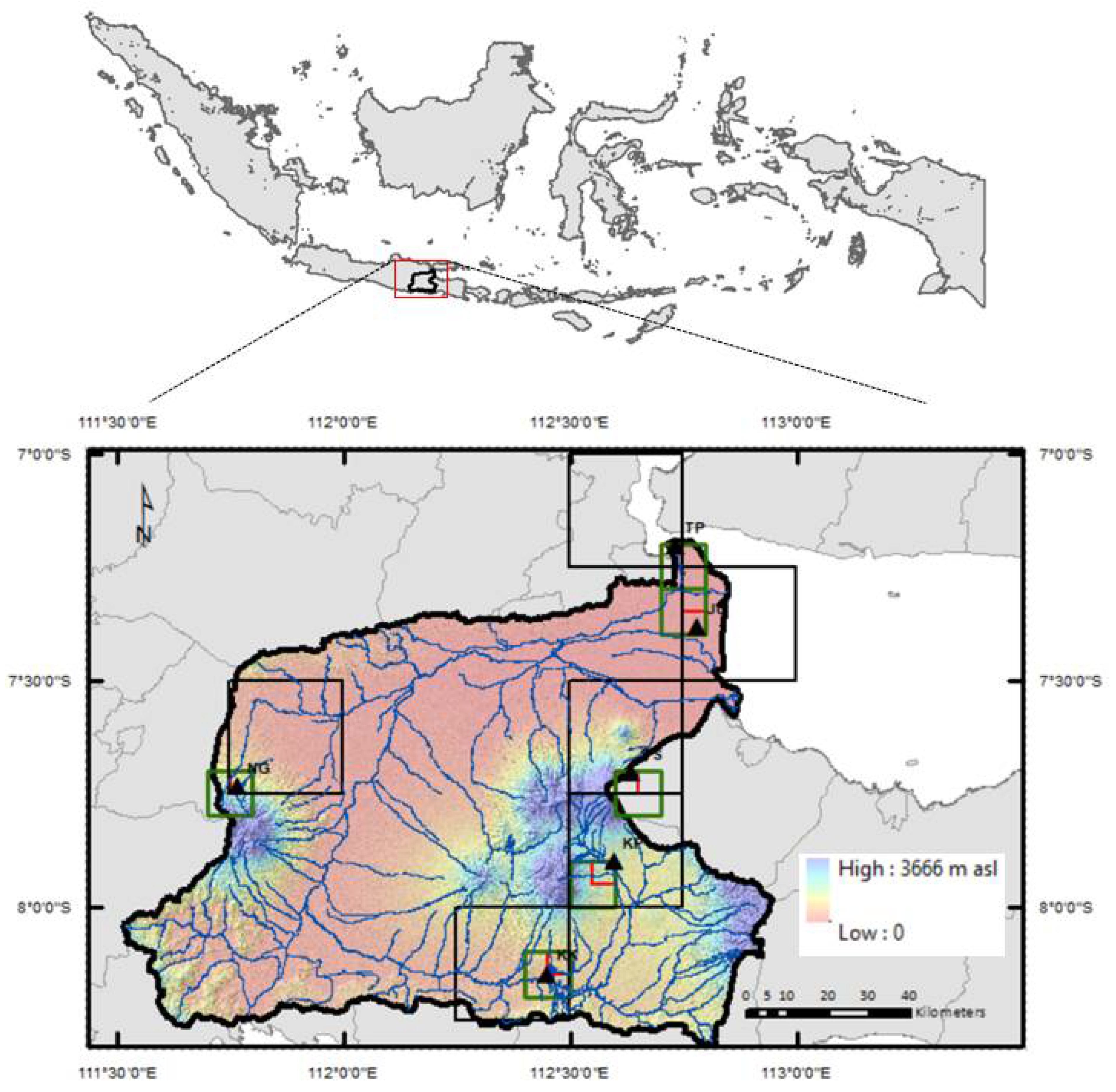
2.1. Study Area

Brantas watershed is a typical humid tropic watershed, with an area of around 11,832 km², and is situated in East Java, Indonesia (Figure 1). It has undergone increasing urbanization and harbors around 21 million dwellers, representing around 14% of the Java island’s population, the most populated island in the country. Brantas is a primary watershed because of its economic and ecological importance to the province. It is also home to 15 cities, municipalities, and regencies, locally termed as kota besar, kotamadya and kabupaten, respectively. Geologically, the Brantas landscape was influenced by the Quaternary Plate tectonics landforms, which are spatially distributed locations on subduction and collision zones caused by lateral movement of the tectonic plates. Active volcanism is associated with belts of ongoing subduction between Asian and Indo-Australian plates. Mountainous ranges are subjected to intense humid tropical weathering processes, erosions, and mass movements. These geomorphology processes create variations of landforms, reflecting differences in the resistance of the bed rock to geological events in the past. With seven mountain complexes (Arjuno-Welirang complex, Semeru-Bromo-Tengger complex, Kelud-Kawi complex, and Ngliman complex) present within the area, Brantas exhibits a gradient in temperature and elevation. The range of elevation spans from 0 to 3666 m asl, with the slope ranging from 0 to 85 degrees, meaning that the region is affected by orographic systems. The annual average rainfall ranges from 1200 to 3600 mm. The monsoonal influence is evident, with Brantas’ climate being classified as Am in Köppen-Geiger’s classification system.

2.2. Satellite Rainfall Data Acquisition and Processing

We reviewed several satellite rainfall products and selected three satellite products, CHIRPS, GPM, and PERSIANN, for several reasons: relatively finer resolution (≤25 km), long coverage (>20 year), available on a daily basis, and currently being operational. We selected three differing resolutions to enable us to obtain information regarding the products’ performances in supporting applications from local to national scales. Despite numerous studies elsewhere, these datasets have never been exclusively assessed for Javanese landscapes. The three datasets are widely used, yet pose their own advantages and limitations.

Table 1. Advantages and limitations of each rainfall dataset.

Dataset	Advantages	Limitations
CHIRPS	Highest resolution, ~5 km, more suitable for detailed assessment in small areas with a short latency. Potential for smaller biases due to its higher resolution [29]	Larger data size per unit area due to higher spatial resolution. The IR brightness temperature-based algorithm included in CHIRPS is insensitive to rain affected by orographic effects, due to its low temperature clouds, and is moderately sensitive to precipitation from typhoon weather systems [30]
GPM-IMERG	GPM-IMERG combines intermittent precipitation estimates from all constellation microwave sensors, IR-based observations from geosynchronous satellites, and monthly gauge precipitation data [31] Available at a 0.1° and half–hourly and hourly temporal scales, respectively, they offer the opportunity for capturing finer local precipitation variations in space and time [32]	Over oceans, it is likely that the performance of IMERG will be better because of better microwave retrieval over the ocean, but poorer over mountainous areas [33] The geostationary IR from IMERG has two main limitations, which are the mismatch between IR-based cloud-top and surface precipitation motions, and the limited latitude coverage (60° N–S) caused by viewing angle limitation [34]
Ground data/rain gauge data	Ground-based rainfall measurements from gauges/radars often provide higher spatial and temporal sampling as well as the most direct measure of rainfall over many regions. Often such data are used for purposes of calibration [35]	Coverage might be limited, unevenly distributed, or sparsely distributed. High potential for recording errors due to lack of maintenance and low-skill gauge operators, and often limited by incomplete or missing data [36]
PERSIANN-CDR	Consistent, long-term data set with more than 30 years of data, updated quarterly [37] Given its coarse resolution, it is relatively suitable for large-scale (continental or national level assessment) and benefitted from smaller data size [38]	CDR version has daily temporal resolution, does not resolve the diurnal cycle, may not record some short-lived, intense events and is not independent of other precipitation estimates. Relies heavily on infrared data—conversion from IR to precipitation rate requires complex algorithm, not quite global (60° S–60° N) [37]

presents an overview of these advantages and limitations.

PERSIANN is a gridded rainfall dataset that is generated at 3-h intervals, with 0.25 × 0.25° lat/lon resolution and is available for regions within 60° N–60° S. PERSIANN’s algorithm relies on an artificial neural network and Infra-Red (IR) brightness temperature. The daily PERSIANN-Climatic Data Record (afterwards called PERSIANN-CDR) is a daily quasi-global product spanning from 1983 to the present (https://www.ncdc.noaa.gov/cdr/atmospheric/precipitation-persiann-cdr). The product is developed by the Center for Hydrometeorology and Remote Sensing at the University of California, Irvine (UC-IRVINE/CHRS) using the Gridded Satellite (GridSat-B1) IR data that are derived from merging ISCCP B1 IR data, along with GPCP version 2.2 [39]. The dataset in Google Earth Engine (GEE) is available in a readily analyzed geo-tiff format for handy interpretation with pixel values representing the amount of daily precipitation in mm. Most of the rainfall gridded data are available in rain rate unit, mm/day. To make it comparable with other datasets, the daily amount of the data was converted to daily rain rate, in mm/day, by a division to one. Given its relative coarseness, PERSIANN is more suitable for large scale assessments, such as at the national and continental level.

The third satellite rainfall data used in this study are Global Precipitation Measurement (GPM), a new generation of satellite precipitation products, which are a follow-up to the TRMM data. The data are available at 0.1° × 0.1° lat/long from 60° N–60° S. Several studies on GPM-IMERG datasets included numerous assessments and applications carried out in several places in China, Egypt, Austria, Singapore, and Peru [9,40,41,42,43]. None of the datasets have been examined for their performance in Indonesia using long-term data. The GPM gridded data were downloaded using the same platform, Google Earth Engine, with the selected gridded data being at the daily calibrated precipitation rate (mm/day) following the protocol from GEE’s catalogue (https://developers.google.com/).

The Climate Hazards Group Infrared Precipitation Satellite (CHIRPS) is a new land-only climatic gridded database for precipitation at a higher resolution (0.05° lat/lon) (https://www.chc.ucsb.edu/data/chirps). It incorporates several information types, such as global climatology, satellite estimates and in situ observations, to create gridded rainfall timeseries suitable for trend analysis and seasonal drought monitoring [29]. The temporal coverage is from 1981 to present, and the spatial resolution is higher, up to 0.05° lat/lon. There have been CHIRPS validation studies across the globe, such as in in Brazil, China, Italy, and Eastern Africa [30,44,45], but there have been none for Indonesian regions. The gridded CHIRPS raster dataset is also downloadable from Google Earth Engine with pixel values in a daily rain rate unit (mm/day).

All the datasets were downloaded on a daily basis from 1 January 1990 to 31 December 2020 using the Google Earth Engine by matching the pixel locations with the rain gauges’ locations. Each of the pixel boundaries of the CHIRPS, GPM, and PERSIANN pixels, where the gauges were located, were uploaded as assets in GEE and were used as the clipping boundaries for extracting the average daily rain rates for each of the corresponding pixel boundaries. The daily data were then exported as csv files for further comparison with the gauges’ daily data.

2.3. Ground Rainfall Data Acquisition and Processing

The ground rainfall data, which were obtained from the six gauges available within the study area, were publicly available rainfall data from Indonesia’s BMKG (local meteorological agency), available from their website (https://dataonline.bmkg.go.id/home). The data were downloaded on a daily basis from 1 January 1990 to 31 December 2020. The data were then examined for their integrity. This included removal of missing values, flag values, and errors based on the BMKG’s data quality categories. The missing values, errors, and invalid measurements were counted. The distribution of samples was summarized in Figure 2 below. The data coverage, as shown in Figure 2, showed that most years have more than 75% daily coverage.

The location of each rain gauge was used as the basis to locate and extract the satellite estimates based on a nearest neighbor approach. This was selected because the resolutions of the satellite estimates are much larger than the point accuracy of the gauge locations. Pixel-to-point method was selected to obtain a pair of daily rainfall data (mm/day) for each of the gauge locations for the whole period (1 January 1990–31 December 2020). Six rain gauges used in this study exhibited differing ecological characteristics. A summary of the gauges is given in the below table (

Table 2. Six gauges’ characteristics.

	Gauge Locations
	JU	KK	KP	NG	PS	TP
Elevation (mean)	2.3	326.4	649.3	584.7	1479.2	4.7
Temperature range (°C)	24–37	26–29	28–31	25–28	17–22	28–38
Wind-speed range (m/s)	2–5	2–5	2–5	2–5	2–5	2–5
PET range (mm/day)	0.6–1.7	0.8–1.7	0.6–1.7	0.8–1.8	0.1–1.8	0.1–1.8
Total annual rainfall (mm)	1567	1846	1576	2059	2373	1286
Average daily rainfall rate (mm/day)	4.8	5.6	5.2	6.2	8.4	4.0

).

2.4. Accuracy Assessment of Three Satellite Rainfall Estimates

Accuracy signifies the closeness of the estimated data to an acceptable standard, which in this case is the rainfall data from the gauges. To obtain information about the performance of satellite rainfall estimates, two types of accuracy assessments were carried out on the pairs of daily rainfall data from the gauges and satellites, namely quantitative and qualitative assessment. The quantitative assessment is useful in providing information about the magnitudes of the rain estimates and its biases, while the qualitative one is useful in depicting the general usability of the satellite rainfall estimates in capturing the rain events.

2.4.1. Quantitative Assessment

Four statistical measures were employed to examine the accuracy of the satellite rainfall data, namely Root Mean Square Error (RMSE), Normalize RMSE (NRMSE), Mean Absolute Error (MAE), and Spearman Correlation Coefficient (CC), as expressed below:

$$\mathrm{RMSE}=\sqrt{\frac{1}{\mathrm{n}}}{\displaystyle \sum }_{\mathrm{i}=1}^{\mathrm{n}}{\left({\mathrm{S}}_{\mathrm{i}}-{\mathrm{G}}_{\mathrm{i}}\right)}^2$$

(1)

$$\mathrm{NRMSE}(\%)=\frac{\mathrm{RMSE}}{\left(\mathrm{Gmax}-\mathrm{Gmin}\right)}\ast 100$$

(2)

$$\mathrm{MAE}=\frac{{{\displaystyle \sum }}_{\mathrm{i}=1}^{\mathrm{n}}\mathrm{abs}\left({\mathrm{S}}_{\mathrm{i}}-{\mathrm{G}}_{\mathrm{i}}\right)}{\mathrm{n}}$$

(3)

$$\mathrm{CC}=\frac{{\left[{{\displaystyle \sum }}_{\mathrm{i}=1}^{\mathrm{n}}\left({\mathrm{S}}_{\mathrm{i}}-\overline{\mathrm{S}}\right).\left({\mathrm{G}}_{\mathrm{i}}-\overline{\mathrm{G}}\right)\right]}^2}{{{\displaystyle \sum }}_{\mathrm{i}=1}^{\mathrm{n}}{\left({\mathrm{S}}_{\mathrm{i}}-\overline{\mathrm{S}}\right)}^2{{\displaystyle \sum }}_{\mathrm{i}=1}^{\mathrm{n}}{\left({\mathrm{G}}_{\mathrm{i}}-\overline{\mathrm{G}}\right)}^2}$$

(4)

where G_i = rainfall from gauge, Si, rainfall from satellite, G_max is maximum observed rainfall from gauge, G_min is minimum rainfall from gauge, $\overline{\mathrm{S}}$ is the mean of satellite rainfall, and $\overline{\mathrm{G}}$ is the mean of satellite rainfall. To obtain insights about the temporal accuracy variability, the accuracy measurements were carried out at four different timespans: daily, monthly, dry season, and wet season. April to September is classified as the dry division, and October to March is classified as the wet division [28].

2.4.2. Qualitative Assessment

To investigate the ability of satellite rainfall data to sense rainfall events, four categorical statistics were calculated and compared through a cross-table of variables meeting certain conditions. The four statistics are “hits (a)”, “misses (c)”, “false (b)”, and “correct negatives (d)”. This approach would allow a decomposition of the categorical bias of each satellite products [16]. The contingency table for the rainfall categories is as below (

Table 3. Cross-table of categorical rainfall measures.

		Rain Gauge (mm/day)
		Rain > 0 mm/day	Rain = 0 mm/day
Satellite estimates	Rain > 0 mm/day	a (hits)	b (false)
	Rain = 0 mm/day	c (misses)	d (correct no rain)

):

The following measures were then calculated from the “a”, “b”, “c”, and “d”:

$$\mathrm{Probability}\mathrm{of}\mathrm{detection}(\mathrm{POD})\mathrm{POD}=\frac{a}{a+c}$$

(5)

$$\mathrm{Frequency}\mathrm{of}\mathrm{hit}(\mathrm{FOH})\mathrm{FOH}=\frac{a}{a+b}$$

(6)

$$\mathrm{False}\mathrm{alarm}\mathrm{ratio}(\mathrm{FAR})\mathrm{FAR}=\frac{b}{a+b}$$

(7)

$$\mathrm{Critical}\mathrm{success}\mathrm{index}(\mathrm{CSI})\mathrm{CSI}=\frac{a}{a+b+c}$$

(8)

In our opinion, the ability of satellite products to detect rain events should also consider the ability to detect no-rain events, and thus we added one indicator as DA, or degree of ability, as expressed below:

$$\mathrm{Degree}\mathrm{of}\mathrm{ability}(\mathrm{DA})\mathrm{DA}=\frac{a+d}{a+b+c+d}$$

(9)

2.5. Association of Errors to Varying Ecological Variables

To examine whether errors from satellite rainfall products are associated with ecological or land characteristic variables, the absolute errors from each satellite product were correlated to several ecological variables, namely, elevation, slope, Normalize Difference Vegetation Index (NDVI) as a surrogate of physical land surface characteristics, wind, and Potential Evapotranspiration (PET) from each station (

Table 4. Types and Source of Ecological Variables.

Dataset	Source	Resolution
Mean and CV of Elevation (AV_EL, CV_EL)	ASTER DEM V2	30 m
Mean and CV of Slope (AV_SL, CV_SL)	ASTER DEM V2	30 m
Mean and CV of NDVI (NDVI)	MODIS	500 m, daily, monthly aggregated
Mean potential evapotranspiration (PET)	MODIS 16-ET	500 m, 8-day, monthly aggregated
Mean wind (Wind)	NOAA AVHRR	5 km, daily, monthly aggregated
Mean temperature (Temp)	MODIS-LST	1 km, daily, monthly aggregated

). The datasets were extracted and downloaded using Google Earth Engine with the satellite pixel boundaries similar to the approach applied in Section 2.2. We used monthly aggregated level data and calculated the Spearman correlation to measure the degree of the association between ecological variables and the magnitude of errors in monthly levels. All the ecological variables or land characteristics were collected from publicly available remote sensing datasets, as below:

2.6. Impacts of Satellite Rainfall Products on Hydrological Response Outputs

2.6.1. Model Description, Input, and Model Setup

Hydrological modeling tools have been widely applied in the investigation into the behavior of hydrological systems [46]. While their advantage is clear, one evident limitation is the reliance on massive climatic data, which are difficult to obtain. Climatic variables were often derived from remote sensing products [47,48]. To understand the influence of using satellite rainfall data to assess the quality of hydrological outputs, we applied a Soil and Water Assessment Tool (SWAT) to a selected sub-watershed which had a long-term discharge of data. The simulation used has been successfully applied to simulate hydrological processes in upper Brantas in our previously published study. The details of the model inputs, setup, and validated parameters were adopted from the validated parameters in this area from the previous study, which were run on a monthly basis (calibration 2003–2008 and validation 2009–2013) [49]. We re-simulated this model into three identical SWAT projects, except for the precipitation inputs, to examine the influence of precipitation data derived from three satellite rainfall estimates on the estimated daily flow. We specifically focused on the selected sub-basin used in the previous study for continuity. We used the sub-basin boundary to extract the daily rainfall data from CHIRPS, PERSIANN and GPM downloaded through the Google Earth Engine as specified in Section 2.2.

The model parameters applied in this study were taken from the previous study, as they had been validated and assessed for their accuracy and sensitivity in detail [49]. In this study, we replicated the SWAT project and created three similar projects with exactly similar inputs and parameters, and therefore the only source of difference was the rainfall data. This approach enabled an examination of the impact of the rainfall data input on the hydrological output performance.

2.6.2. Model Performance Evaluation

To evaluate the accuracy of the flow outputs from the three models above, compared to the observed flows, SWAT-CUP computed the accuracy metrics R² and a Nash–Sutcliffe Efficiency (NSE) coefficient as below:

$$R^2=1-{[\frac{{{\displaystyle \sum }}_{i=1}^n\left(Q_{obs}-Q_{pred}\right)\left(Q_{pred}-\overline{Q_{pred}}\right) }{{\left({{\displaystyle \sum }}_{i=1}^n{\left(Q_{obs}-\overline{Q_{obs}} \right)}^2\right)}^{0.5} {\left({{\displaystyle \sum }}_{i=1}^n{\left(Q_{obs}-\overline{Q_{obs}} \right)}^2\right)}^{0.5}} ]}^2$$

(10)

$$\mathrm{NSE}=1-\frac{{{\displaystyle \sum }}_{\mathrm{i}=1}^{\mathrm{n}}{\left(Q_{pred}-Q_{obs}\right)}^2}{{{\displaystyle \sum }}_{\mathrm{i}=1}^{\mathrm{n}}{\left(Q_{obs}-\overline{Q_{obs}}\right)}^2}$$

(11)

where Q_obs is the observed value, Q_pred is the simulated value, $\overline{Q_{obs}}$ and $\overline{Q_{pred}}$ are the means of the observed and simulated values, respectively, and n is the number of observations. The coefficient of determination (R²) quantifies the proportional variation in the predicted variable, explained by the observed variable, and indicates the linear relationship between the predicted and observed variables. The Nash-Sutcliffe Efficiency (NSE) determines the relative magnitude of the residual variance compared to the observed data [50]. It ranges from −∞ to 1 with 1 representing a perfect agreement between the simulated and measured values.

In addition to measuring the accuracies, we also quantified the uncertainties associated in the modeling. The uncertainties in hydrological modeling might originate from three possible sources: input data, such as the rainfall and temperature data that can affect the simulation results directly (i.e., surface runoff); model structure, which is mainly caused by the assumptions and simplification of the model; and model parameters [51,52,53]. Among these groups, models’ parameters were considered as the relatively easily controlled group, through a calibration step, and input datasets were perceived as the biggest source of uncertainties [13,54]. To quantify such uncertainty, we used the SWAT Calibration-Uncertainty Program (SWAT-CUP) accompanied by the SWAT modeling. We selected the widely applied program sequential uncertainty fitting SUFI-2 [53,54]. Using a Bayesian framework, SUFI2 computes the uncertainties through the sequential and fitting processes. In SUFI2, the parameter uncertainty is calculated from all sources such as input variables (e.g., rainfall data, temperature, and land use) and model structure. SWAT-CUP/SUFI-2 calculated several measures in addition to R² and NSE. The P-factor represents the degree to which all uncertainties accounted for is quantified, accounting for the percentage of the observed data within the 95% prediction uncertainty (95PPU). Another measure is the R-factor, a measure quantifying the strength of the uncertainty analysis, which is manifested as the average thickness of the 95PPU band divided by the standard deviation of the observed data. A higher P-factor (close to 1) and smaller R-factor (close to 0) is expected [55]. By comparing the R2, NSE, P-factor and R-factor, we deduced the relative performance of each satellite rainfall estimate for hydrological modeling.

3. Results

3.1. Accuracy Assessment Results

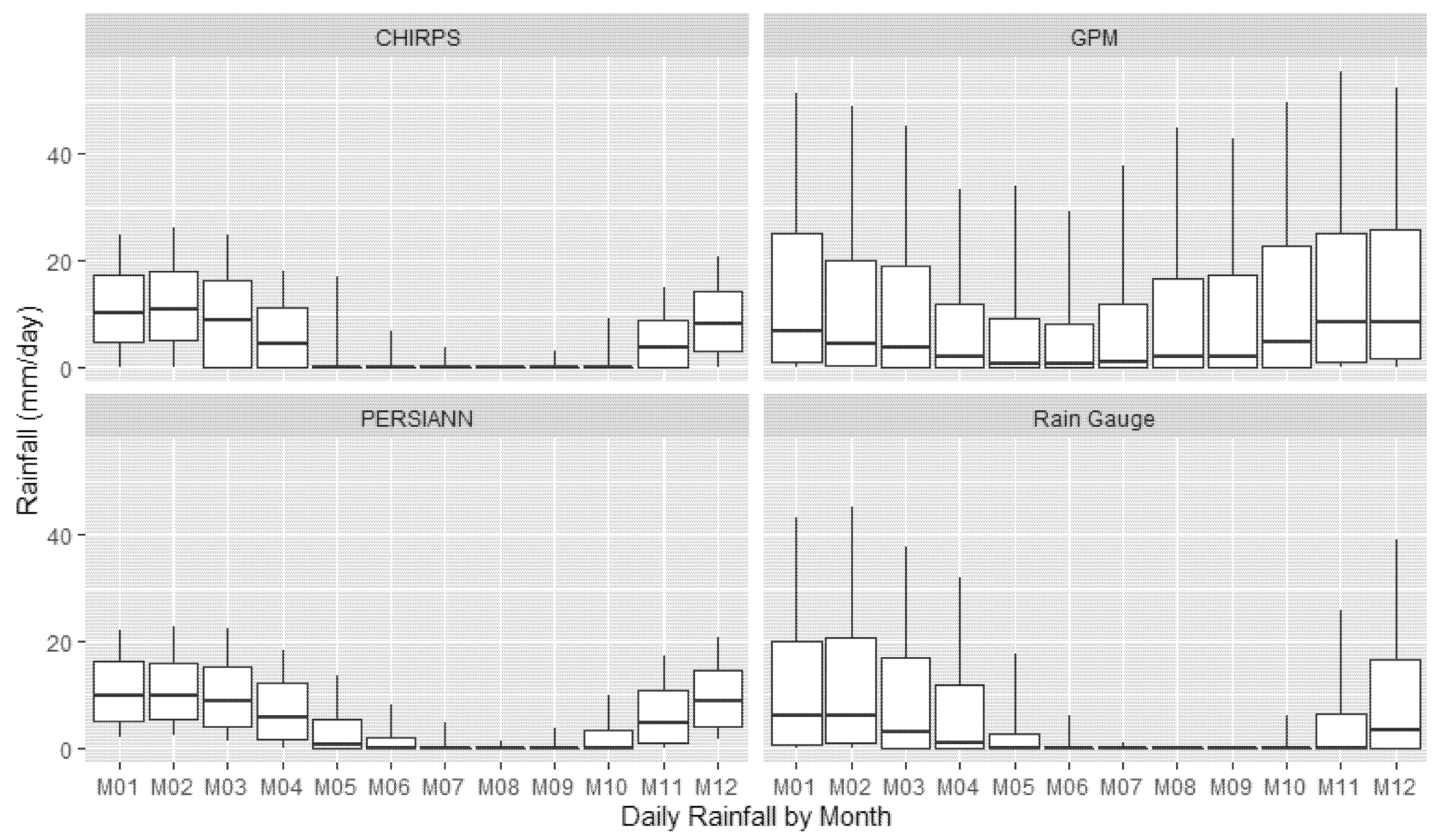
3.1.1. Descriptive Statistics of Satellite Rainfall Data

The results of rainfall extraction from satellite data and comparison with ground data is presented in Figure 3, Figure 4 and Figure 5.

The scatter plots show that CHIRPS and PERSIANN mainly underestimated for the rainfall higher than 100 m/day, especially in Nganjuk (NG), Pasuruan (PS), Juanda (JU), and Tanjung Perak (TP). GPM appears to be relatively more sensitive to ground rainfall variations.

Despite poor visual agreement in Figure 3, Figure 4 shows that satellite products have good visual seasonal patterns. It appears that after removing outliers, CHIPRS shows better seasonal patterns than GPM and PERSIANN. In dry seasons, CHRIPS appears to show a rainfall variability which is as visually good as the gauge’s rainfall, however, in wet seasons (Figure 4B), when outliers are considered, CHIRPS cannot detect rainfall over 100 m/day. Through this figure, GPM overestimates the observation in both dry and wet season.

Monthly-based daily rainfall distribution in Figure 5 provides more detailed information about the temporal patterns of satellite products. Figure 5 shows that all rainfall estimates from the three sources follow the pattern of the gauges’ rainfall. The seasonal patterns are clearer in CHRIPS and PERSIANN, while estimates from GPM clearly show overestimation from month to month, as also shown by Figure 4B.

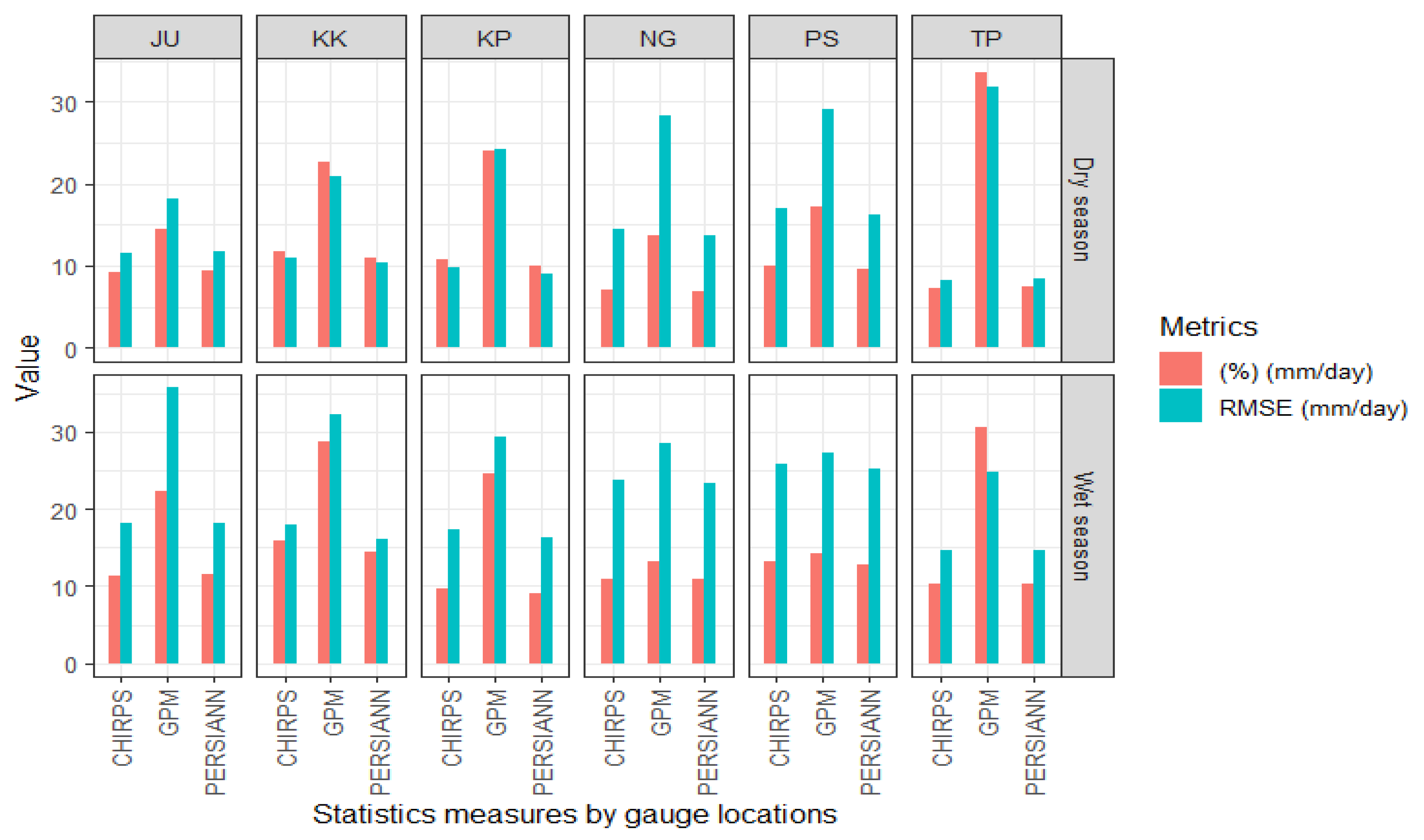
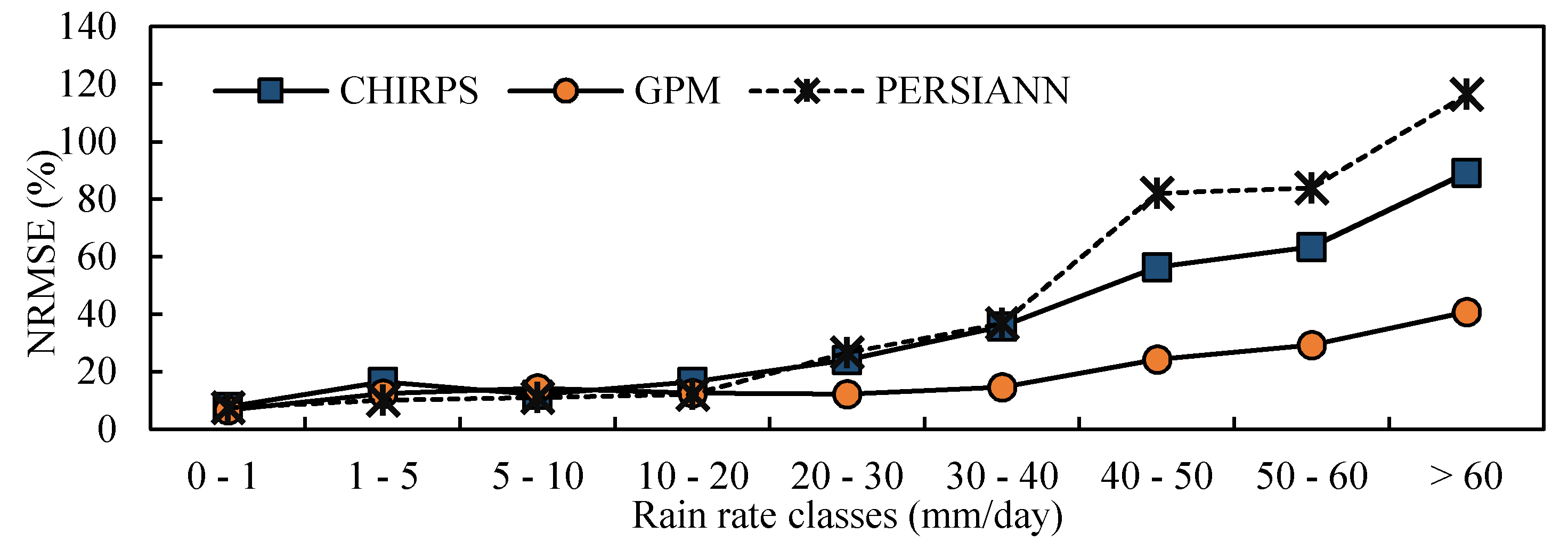
3.1.2. Quantitative Accuracy Assessments

A summary of quantitative accuracy assessments of three satellite products is presented in

Table 5. Summary of quantitative accuracy measures from three satellite rainfall products. Data calculated with outliers included.

Level	Dataset *	CHIRPS				GPM				PERSIANN
		RMSE	CC	MAE	NRMSE	RMSE	CC	MAE	NRMSE	RMSE	CC	MAE	NRMSE
Daily (mm/day)	All-combined	16.56	0.28	7.99	7.68	27.85	0.28	14.06	12.93	16.15	0.29	7.95	7.49
	JU	15.17	0.28	7.15	9.52	28.19	0.22	12.93	17.70	15.28	0.26	7.54	9.59
	KK	14.95	0.31	8.40	13.35	27.30	0.37	13.17	24.38	13.62	0.32	7.47	12.16
	KP	14.07	0.23	7.45	7.82	27.02	0.21	14.45	22.52	13.21	0.26	7.05	7.34
	NG	19.72	0.28	9.24	9.15	28.36	0.37	13.45	13.16	19.24	0.31	9.13	8.93
	PS	21.93	0.26	11.20	11.13	28.09	0.30	16.03	14.78	21.32	0.31	10.73	10.82
	TP	11.80	0.36	5.56	8.28	28.63	0.23	15.40	30.30	11.86	0.35	6.05	8.32
Total Monthly rainfall (mm)	All-combined	139.20	0.79	83.37	10.09	252.64	0.84	181.41	22.74	135.86	0.79	83.63	9.85
	JU	104.93	0.86	67.17	11.84	258.38	0.89	188.20	29.16	97.83	0.84	65.72	11.04
	KK	113.58	0.77	86.85	21.59	294.48	0.90	230.71	55.98	80.04	0.85	54.19	15.22
	KP	88.91	0.81	61.47	13.72	314.92	0.84	230.30	61.39	86.54	0.81	60.16	13.36
	NG	178.93	0.79	111.87	18.04	192.93	0.94	143.92	18.90	169.81	0.84	110.60	17.12
	PS	221.90	0.84	151.26	16.08	159.65	0.90	117.09	14.37	224.26	0.87	153.22	16.25
	TP	60.69	0.88	39.16	11.92	319.88	0.90	255.40	67.51	66.91	0.87	49.12	13.16
Daily in wet season	All-combined	19.91	0.22	11.44	9.24	30.77	0.24	16.77	14.28	19.51	0.22	11.35	9.05
	JU	18.13	0.22	10.23	11.38	35.66	0.16	19.84	22.39	18.24	0.19	10.79	11.45
	KK	17.89	0.21	11.78	15.98	32.14	0.29	18.70	28.70	16.16	0.23	10.29	14.43
	KP	17.23	0.16	10.86	9.57	29.37	0.18	16.59	24.47	16.30	0.16	10.23	9.06
	NG	23.73	0.21	13.19	11.01	28.48	0.37	13.77	13.21	23.41	0.22	13.19	10.86
	PS	25.79	0.19	15.36	13.09	27.18	0.29	15.28	14.30	25.29	0.22	14.80	12.84
	TP	14.56	0.32	8.31	10.22	24.76	0.31	12.60	30.57	14.57	0.30	8.77	10.23
Daily in dry season	All-combined	12.26	0.22	4.48	6.13	24.51	0.30	11.28	11.90	11.85	0.26	4.53	5.93
	JU	11.55	0.26	4.12	9.20	18.24	0.22	6.24	14.54	11.73	0.24	4.39	9.34
	KK	10.99	0.37	4.80	11.82	20.99	0.45	7.31	22.57	10.28	0.36	4.49	11.05
	KP	9.76	0.19	3.91	10.85	24.27	0.23	12.16	24.03	8.97	0.23	3.79	9.97
	NG	14.41	0.25	5.12	6.99	28.23	0.37	13.12	13.71	13.69	0.32	4.96	6.84
	PS	17.00	0.21	6.86	10.06	29.02	0.29	16.84	17.17	16.24	0.30	6.54	9.61
	TP	8.27	0.27	2.88	7.27	31.74	0.17	17.94	33.59	8.47	0.31	3.43	7.44

* All combined dataset represents taken from all six gauge’s locations (JU, KK, KP, NG, PS, and TP).

, covering accuracy assessment results by season, monthly rainfall aggregates, and the gauges’ individual locations. From Table 5, we can see that CHIRPS and PERSIANN have relatively similar performances, given the similar values of RMSE, MAR, CC, and NRSME, as shown in the combined daily data. The errors were evidently larger in the wet season, especially from GPM, whose NRMSE can reach 30%. Daily error ranges from CHIRPS and PERSIANN were relatively similar at 8–13% of NRSME (CC 0.28–0.35). Despite the weak performance of the daily data, monthly aggerated data show an improved association (CC 0.79–0.91) for all satellites. If we consider geographic variations, there have been varying performances from six locations, and apparently no observable patterns of errors with gauge locations. A more detailed comparison for each gauge location is presented in Figure 6. In all stations, GPM consistently exhibits the largest error compared to CHRIPS and PERSIANN.

To examine the error distribution, error histograms were created, as in Figure 7. The figure allows for the assessment of whether the errors were distributed normally or not. This can also infer if the satellite data experience a systematic error. As shown in Figure 7, the errors of three satellite products were normally distributed. It is also evident that wet season errors are the primary source of total errors.

Despite the normal error distributions as shown in Figure 7, the data show that the magnitude of errors are related to the magnitude of rain rates. Figure 8 shows the patterns between rain rate classes on the ground and magnitude of errors in terms of RMSE and NRMSE. Apparently, the error increases exponentially for higher rainfall rates. In rain rate classes of more than 20 mm/day, the RMSE values jump to higher than 10 mm/day, and even reach higher than 50 mm/day when rain rates are very high (>60 mm/day).

3.1.3. Quantitative Accuracy Assessments

A summary of the quantitative accuracy assessments of the three satellite products is presented in

Table 6. Categorical accuracy measures of three satellite products.

Source	Dataset	Accuracy Measure
		POD	FOH	FAR	CSI	DA
CHIRPS	All-combined	0.70	0.68	0.32	0.52	0.74
	Wet season	0.78	0.72	0.28	0.60	0.70
	Dry season	0.46	0.53	0.47	0.33	0.78
GPM	All-combined	0.96	0.54	0.46	0.52	0.63
	Wet season	0.98	0.53	0.47	0.53	0.59
	Dry season	0.96	0.54	0.46	0.52	0.63
PERSIANN	All-combined	0.91	0.60	0.40	0.57	0.72
	Wet season	0.76	0.46	0.54	0.41	0.74
	Dry season	0.97	0.66	0.34	0.65	0.69

below.

Despite the poorer performance of GPM’s rainfall data in terms of RMSE, MAE, and NRMSE, the GPM data show a better performance in detecting rain events, as shown by its consistent highest POD values in all dataset types (0.96–0.98). This confirms the finding from Figure 3 where GPM was able to show a sensitivity to rain events. However, the FOH and FAR scores of CHIRPS were the best, especially in all combined and wet season data, with the values being generally lower than 0.60. CSI integrates the comprehensive measures of accurate prediction, false prediction, and missing precipitation. The CSI scores varied by season and showed no clear observed patterns, with poor values lower than 0.6. The degree of ability shows that CHIPRS and PERSIANN are relatively similar (ranging from 0.6 to 0.8), which supports the similarity of quantitative accuracy measures in Table 4. The considerable differences in POD and DA suggests the low ability of the satellite-based rainfall estimates, especially in GPM, to match ground conditions where no rain is observed.

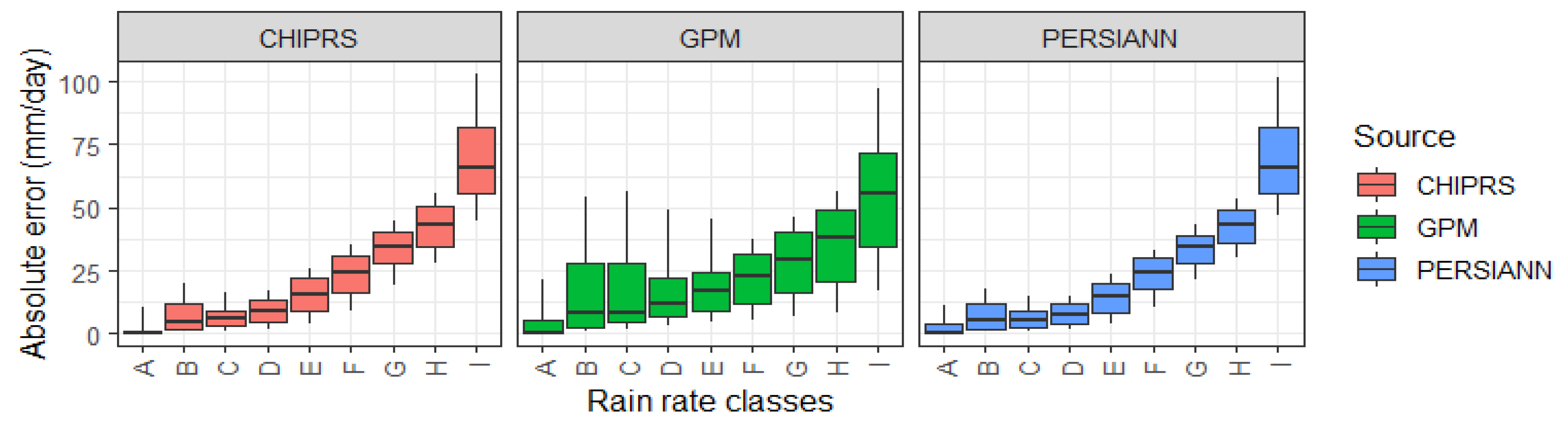
3.2. Influence of Varying Ecological Variables to Errors of Satellite Products

The Spearman correlation results of the errors and corresponding ecological conditions of gauges were presented in

Table 7. Correlation between absolute errors and ecological variables *.

	CHIRPS	GPM	PERSIANN
Cv_NDVI	0.04	−0.03	0.05
Av_NDVI	−0.05	0.16	−0.10
PET	−0.48	−0.01	−0.54
Wind	−0.39	0.14	−0.39
Temp	−0.19	0.21	−0.06
Av_Slope	0.29	0.16	0.29
Cv_Slope	−0.19	−0.17	−0.17
Av_Elevation	0.22	0.20	0.21
Cv_Elevation	−0.14	0.01	0.01

* bold are statistically significant (p < 0.05).

. For elevation, slope and NDVI, we included the coefficient of variation (CV) in addition to the mean values of the data within the satellite pixel boundaries. This is to examine if landscape variability also influences the rainfall estimates.

The correlation values in Table 6 suggest that landscape variables influence the quality of rainfall estimates. From the table, we can observe that the magnitude of errors have some association with the ecological variables or land characteristics. In CHRIPS and PERSIANN data, the association of the absolute errors were found to be significant with the PET and with the average slope within the satellite rainfall pixel boundaries. In brief, larger errors were inversely associated with magnitude of PET and wind, with a negative correlation of −0.48 and −0.39 (for CHIRPS), and −0.54 and −0.39 (for PERSIANN). Apart from climatic variables, the slope, on the other hand, shows that higher average slopes are associated with larger errors, with a correlation of 0.29 for CHIRPS and PERSIANN. Considering the elevation, higher elevation areas tend to pose larger errors, as shown by the positive relationship between the magnitude of errors and all three satellite rainfall products (r = 0.20–0.22). On the other hand, slope variations as a proxy for the topographic condition did not significantly link to the magnitude of errors. Interestingly, as we expected to represent land cover variability within the pixel boundary, both the average and CV of NDVI from the three rainfall estimates showed a very weak association with the error magnitudes (r = −0.10~0.05).

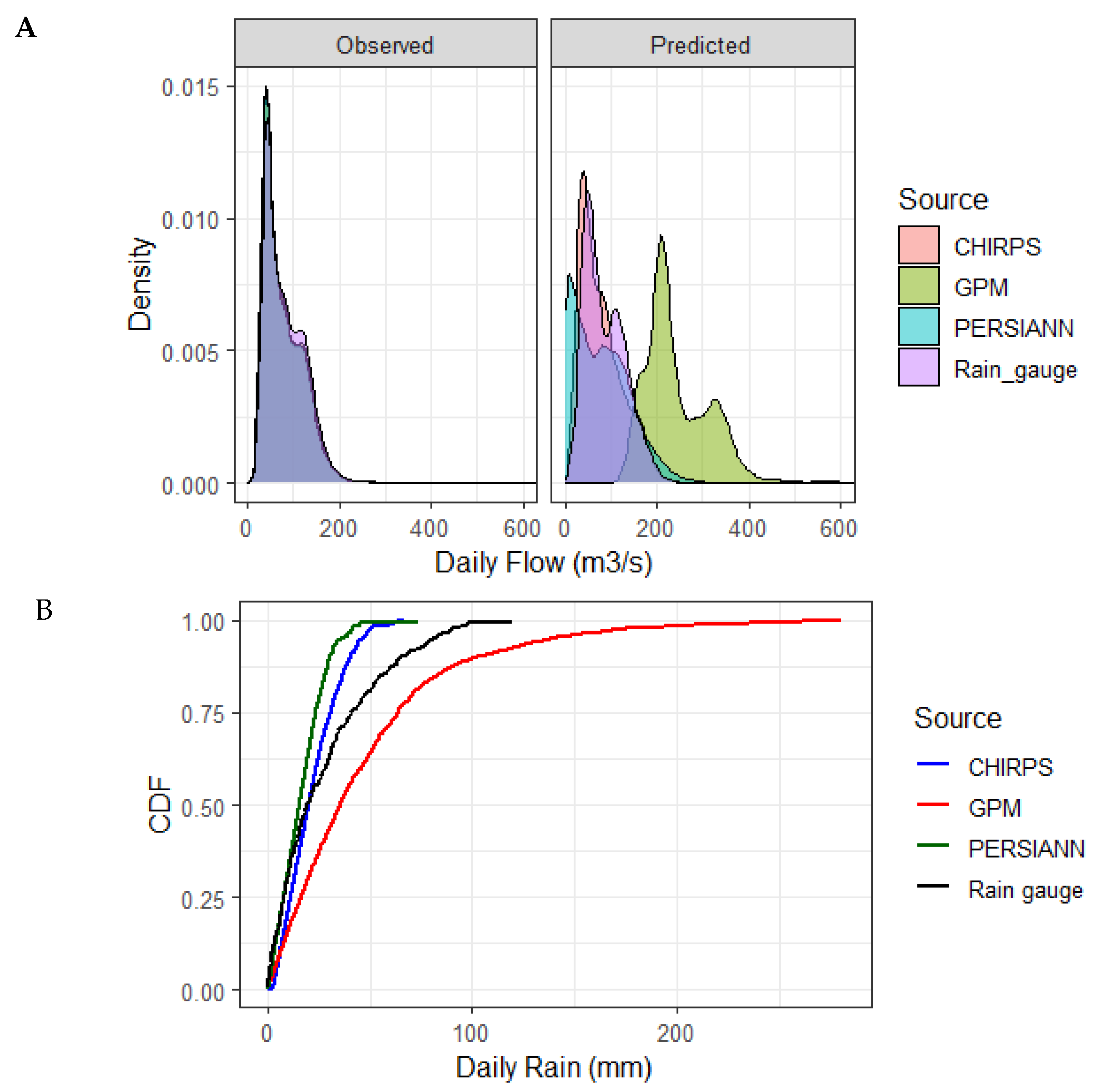
3.3. Assessment of Satellite Products as Inputs for Hydrological Modeling

3.3.1. Accuracy and Uncertainty Performance of the SWAT Models

The SUFI-2 results from the three SWAT models using three satellite rainfall estimates, compared to that of the rain gauges, is presented in

Table 8. Accuracy and uncertainty of SWAT daily models from four rainfall sources.

Dataset	Calibration (2003–2008)				Validation (2009–2013)
	R2	NS	p-Factor	r-Factor	R2	NSE	p-Factor	r-Factor
Rain gauge	0.75	0.74	0.97	1.96	0.74	0.73	0.93	0.94
CHIRPS	0.59	0.54	0.97	1.96	0.62	0.55	0.95	2.22
GPM	0.28	−13.58	0.33	4.49	0.37	−21.44	0.33	4.97
PERSIANN	0.47	0.35	0.92	1.7	0.61	0.55	0.88	1.84

below. From this, it was expected that three satellite-based rainfall inputs did not produce satisfactory results in both the calibration and validation period. The R² and NS, as the accuracy performance for these datasets, are relatively low (R²: 0.28–061 and NS: −21.44 to 0.55). These values are quite different from those gained from the rain gauge data (R²: 0.28–061 and NS: −21.44 to 0.55). Compared to two other satellite products, CHIRPS consistently outperformed the GPM and PERSIANN data, with R² and NS vales being the highest (R²: 0.59–0.62 and NS: 0.54–0.55). The values between calibration and validation are relatively similar, indicating no signs of over-fitting. Regarding the daily timespan, the NS values from the three satellite products were considered to be good, as they are comparable to the satisfactory monthly performance standards [56].

The estimated daily flows plotted against 1:1 line as in Figure 9 reveals the degree of accuracy from each rainfall datasets. Obvious overestimation was found from GPM-based flow estimates. Visually, CHIRPS and PERSIANN show relatively better estimates with narrow confidence interval bands, and almost all observations were within their 95% prediction intervals. GPM, as shown in Table 8, produced the lowest p-factor value (0.33) and r-factor values (4.49–4.97). These measures reveal that flows estimated from SWAT models using GPM data suffer the highest uncertainty. The uncertainty is higher for the flows higher than 200 m3/s, as shown by the increased deviation from both the prediction and confidence interval bands.

Further analysis reveals that the distribution of the estimated flow from CHIRPS is most similar to the estimated flow resulted from the rain gauge data (Figure 10A), especially to the flow with the range of 0–200 m³/s. The cumulative distribution of rainfall inputs (Figure 10B) clearly shows the similarity of CHIRPS and the rain gauge data for lower daily rain ranges (0–25 mm). Given the similarity in model structure, model parameters, and other model inputs (i.e., soil, land cover, and other climatic data), larger errors and higher uncertainty from GPM-based flow apparently originated from the larger deviation, as well as overestimation of the rainfall data as shown in Figure 10B.

The daily performances for the three satellite rainfall products were not satisfactory, as shown by the low R², NS, p-factor, and r-factor. However, the accuracy might be reduced, as well as the increased uncertainty for the application at a monthly basis. The monthly aggregated flow estimates from the daily data showed that R² and r increased drastically to around 0.6 and 0.9 (complete data not shown for brevity).

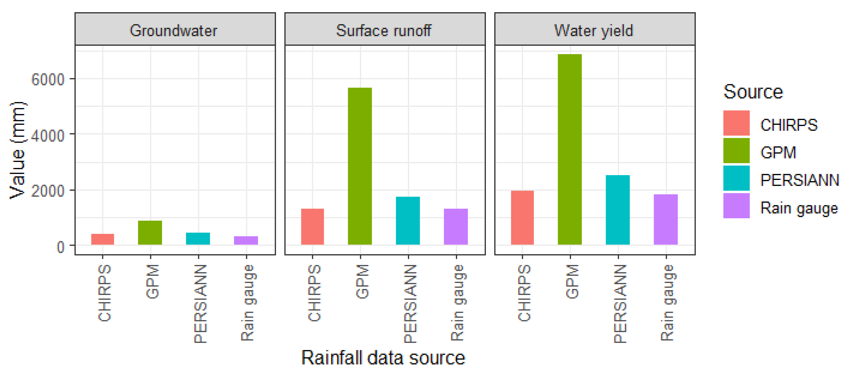
3.3.2. Impacts on Water Balance Components

Result show that, despite relatively good R² values at a monthly level, the three satellite products show negative NSE values, indicating a poor predictive ability. The error from flow data generated from satellite products in SWAT modeling propagated to the subsequential products, which are water balance components. The comparison of water balance components simulated for the year of 2010 is given in Figure 11 below.

The results show that SWAT modeling using rainfall satellite products did not produce very satisfactory results. All water balance components from the three satellite rainfall products show relatively higher than those from the rain gauge. At annual level, the simulated water balance components for the year of 2010 showed different results, as expected. GPM shows a clear overestimation of groundwater, surface runoff, and water yield, with ratio values higher than two. CHIPRS was relatively better compared to GPM and PERSIANN in terms of groundwater. The ratio values of CHIRPS for these two components were relatively close to 1.00. The overestimation and underestimation reflected as a ratio to values from rain gauge data were given in

Table 9. Ratio of water balance components of satellite data products compared to those of rain gauge.

Component	Ratio to Gauge Value
	CHIRPS	GPM	PERSIANN
Surface runoff	1.02	4.35	1.34
Groundwater	1.32	2.87	1.12
Water yield	1.08	3.80	1.40

.

Table 9 shows that the satellite-based rainfall estimates might be inaccurate for the analysis at a daily basis. However, aggregated estimates at an annual level would improve the usability of the satellite rainfall products, especially the CHIRPS’ data, as shown by its ratio values being close to one, the values of the estimates from the rain gauge data.

4. Discussion

In this study, we assessed the performance of the three globally used daily satellite rainfall products, which had varied spatial resolutions, using long-term ground rainfall data from 1990 to 2020. The ground rainfall data came from six varying locations and had similar traits in wind and evapotranspiration statistics, but relatively different traits in terrain and temperature characteristics. Overall, the performance of the three daily satellite rainfall products were not satisfactory, given only CC of 0.22–0.36 at combined daily data. The RMSE and NRMSE values were also not very good, with ranges between 11–21 mm/day and 7–30%, respectively. As expected, the errors in the wet season are larger than in the dry season due to larger rain magnitudes. These results are comparable to those from other tropical studies, such as in Bali [17], but are somewhat better than in tropical Malaysia [57].

In all gauges, both CHIRPS and PERSIANN, despite their relatively better RMSE than that of GPM (Table 4), show a tendency to underestimation (Figure 3). This underestimation was also found in tropical parts of Brazil [58]. These two products are less capable in capturing high rainfall rates. Figure 8 confirms this finding, where the errors of CHIRPS and PERSIANN are exponentially larger with the increase in rainfall rates, mainly higher rates (>20 mm/day). The inability of satellite products to sense high rain rates was probably due to the presence of rainfall/hydrology extremes [40,59].

As opposed to other studies, which show substantial spatial differences in the performance of satellite rainfall data, this study shows that among six locations, there have been no distinct differences in error patterns. This could partially be attributed to the scale of assessment, which is only within 11,000 km², so that the extreme spatial climatic variations within the area were not found. The only location that almost consistently has the largest error is the PS location (>1470 m above sea level). Mountainous terrain can introduce a significant effect to variations of rainfall due to the generation of local wind currents, producing orographic impacts in tropics, especially those close to the maritime region (e.g., [60,61]). This was probably due to the potentially strongest orographic influence in this location. While a study in Bali [17] shows that the land-water interface might contribute to the errors, this study shows that two locations, JU and TP, that have considerably close proximity to coastal areas (~2 km), do not exhibit major difference in performance. This was due in part to the fact that the number of gauges used in this study is limited, and therefore cannot sufficiently represent rainfall variability within the pixel boundary. Discrepancies between satellite products and gauge measurements, therefore, do not necessarily indicate satellite retrieval errors, but instead can originate from low density or nonuniform gauge coverage.

The categorical accuracy assessments reveal that GPM has the highest ability to detect (highest POD), however CHIRPS is more consistent, given its higher FOH, lower FAR, and higher agreement (DA). GPM shows its superiority in sensing wetter climates where rain events are evident, rain-rate magnitudes are high, and rain events are very extreme [31]. This information would offer an opportunity for the GPM to evaluate the spatial rainfall variability in tropical humid regions, especially in Indonesia, which might experience unexpected climate change, and are predicted to be much wetter and exposed to higher incidents of weather extremes [62].

Evaluation results of the relationship between errors and physical variables or land characteristics of the locations show that errors are larger in areas that have higher average elevation and steeper slopes. This suggests that accuracy decreases in the regions that have higher altitudes and topographic gradients. This could potentially be linked to the fact that higher elevation areas are associated with mountainous regions, where orographic influence is stronger [63]. In addition, larger errors can also be linked to the wind and evapotranspiration, where faster winds and higher evapotranspiration are associated with higher precipitation [64], thus introducing larger errors at higher rain rates. The larger errors in lower PET regions in tropics might be attributed to the ability of the algorithms of the satellite rainfall products. The ability of a satellite to detect and estimate the rate of rain is affected by the complex relationship between rain rates and brightness temperatures, which needs adjustment based on the evaporated water and relative humidity [65]. Larger errors in lower PET regions might be attributed to these variables, since these two variables are associated with the evapotranspiration and wind in the atmosphere. With regards to the land physical cover, interestingly, all three rainfall datasets did not show any observable association to the CV of NDVI values within the corresponding pixel boundaries. While the CV of NDVI values can provide an inference about variations of land-uses, these findings suggest that within the resolution of interest (5 km~25 km), the variations of land-uses/land-cover should not be a concern. Among the three rainfall products, GPM is the only satellite product whose errors show correlation with NDVI (r = 0.16). NDVI values represent the density of vegetative cover. Denser coverage induces infrared scattering from leaf structures. In addition, higher NDVI values are usually forested areas where precipitation is high. GPM’s algorithm is designed to intercalibrate, merge, and interpolate “all” satellite microwave rainfall estimates, in conjunction with microwave-calibrated infrared (IR) satellite estimates and precipitation gauge analysis [66]. Forest areas are mostly located in higher elevations, sparsely gauged or even ungauged, and often marked with high precipitation. Apart from the ground condition, the weakness of IR-based algorithms in the satellite rainfall estimate, where cloud thickness and cloud top temperature as estimated by the IR, do not always convey with the amount of rainfall. On the other hand, the microwave-based algorithms are also affected by water vapor, cloud liquid, oxygen, surface temperature, and the surface emissivity, which makes it very difficult to differentiate rain from the background, especially in the low rain regime [65]. This combined effect could potentially lead to an association between vegetation cover and errors in rainfall estimates.

This study expanded the assessment of rainfall potentials to hydrological applications. Findings reveal that CHIRPS performed better than GPM and PERSIANN products, delivering generated daily flow with high R² and highest NSE value (R² = 0.59–0.62, NS = 0.54 and 055). This indicates that CHIRPS data has a slightly better ability for hydrological modeling. Table 8 shows that ratios of CHIRPS and PERSIANN for three water balance components are generally better (close to one). The performance from CHIRPS for hydrological modeling is apparently influenced by its finer spatial resolution and station-based interpolator integrated in the algorithms. The results support the potential of CHIRPS for being complementary of rainfall gauge data. While for PERSIANN, it should be noted that PERSIANN’s resolution is 25 km², which probably is not suitable to support the hydrologic applications at the sub-catchments level, which are essential to sustainability resources, disaster management and environmental safety. While GPM, despite its better ability for rain event detection, is too poor to apply the datasets as a surrogate to ground rainfall data due to its extreme overestimation (3–4 times larger than gauge data). Some studies show the potential ways of improving the usability of satellite-based rainfall data. These include a blended method of interpolation and correlation [67], machine learning [68], and correction of orographic influence when applying hydrological modeling [69]. While these approaches were beyond this study, the findings from the study provide insight on the potential of satellite-based rainfall data for hydrological application in a humid tropic country, especially in Indonesia.

5. Conclusions

In this study, we evaluated three satellite rainfall products using long-term daily rainfall data (1990–2020) from six locations in a humid tropic watershed. Based on numerical (quantitative) accuracy measures, GPM is consistently the product with the largest errors in all selected timespans (daily, monthly, and seasonal), while CHIRPS and PERSIANN show similar degrees of performance. However, based on categorical measures, CHIRPS shows relatively consistent performance, as shown by its high POD, FOH, DA and low FAR. On the other hand, GPM shows better sensitivity in capturing rainfall variability, especially during high rainfall events (>40 mm/day). This means that s GPM has more potential for applications related to extreme rain events and hazard assessment. Terrain physical conditions, such as wind, slope, and evaporations, exhibit a degree of association with the magnitude of errors. This information provides insight about future potential satellite data calibration and downscaling efforts. Examination into hydrological modelling shows that CHIRPS slightly shows the best ability to model monthly flow and water balance at a finer resolution, followed by PERSIANN, and GPM being the worst. However, its coarse resolution impedes PERSIANN applications for local and regional analysis supporting watershed management.

References

1. Konapala, G.; Mishra, A.K.; Wada, Y.; Mann, M.E. Climate change will affect global water availability through compounding changes in seasonal precipitation and evaporation. Nat. Commun. 2020, 11, 3044. [Google Scholar] [CrossRef]
2. Gherardi, L.A.; Sala, O.E. Effect of interannual precipitation variability on dryland productivity: A global synthesis. Glob. Chang. Biol. 2019, 25, 269–276. [Google Scholar] [CrossRef] [Green Version]
3. Verón, S.R.; de Abelleyra, D.; Lobell, D.B. Impacts of precipitation and temperature on crop yields in the Pampas. Clim. Chang. 2015, 130, 235–245. [Google Scholar] [CrossRef] [Green Version]
4. Terribile, F.; Agrillo, A.; Bonfante, A.; Buscemi, G.; Colandrea, M.; D’Antonio, A.; De Mascellis, R.; De Michele, C.; Langella, G.; Manna, P.; et al. A Web-based spatial decision supporting system for land management and soil conservation. Solid Earth 2015, 6, 903–928. [Google Scholar] [CrossRef] [Green Version]
5. Ji, T.; Yang, H.; Liu, R.; He, T.; Wu, J. Applicability analysis of the TRMM precipitation data in the Sichuan-Chongqing region. Prog. Geogr. 2014, 33, 1375–1386. [Google Scholar]
6. Ly, S.; Charles, C.; Degre, A. Geostatistical interpolation of daily rainfall at catchment scale: The use of several variogram models in the Ourthe and Ambleve catchments, Belgium. Hydrol. Earth Syst. Sci. 2011, 15, 2259–2274. [Google Scholar] [CrossRef] [Green Version]
7. Mair, A.; Fares, A. Comparison of rainfall interpolation methods in a mountainous region of a tropical island. J. Hydrol. Eng. 2011, 16, 371–383. [Google Scholar] [CrossRef]
8. Chowdhury, M.A.I.; Kabir, M.M.; Sayed, A.F.; Hossain, S. Estimation of rainfall patterns in Bangladesh using different computational methods (arithmetic average, thiessen polygon and isohyet). J. Biodivers. Environ. Sci. 2016, 8, 43–51. [Google Scholar]
9. Zubieta, R.; Getirana, A.; Espinoza, J.C.; Lavado-Casimiro, W.; Aragon, L. Hydrological modeling of the Peruvian–Ecuadorian Amazon Basin using GPM-IMERG satellite-based precipitation dataset. Hydrol. Earth Syst. Sci. 2017, 21, 3543–3555. [Google Scholar] [CrossRef] [PubMed] [Green Version]
10. Gebremichael, M.; Bitew, M.M.; Hirpa, F.A.; Tesfay, G.N. Accuracy of satellite rainfall estimates in the B lue N ile B asin: L owland plain versus highland mountain. Water Resour. Res. 2014, 50, 8775–8790. [Google Scholar] [CrossRef]
11. Syed, K.H.; Goodrich, D.C.; Myers, D.E.; Sorooshian, S. Spatial characteristics of thunderstorm rainfall fields and their relation to runoff. J. Hydrol. 2003, 271, 1–21. [Google Scholar] [CrossRef] [Green Version]
12. Fekete, B.M.; Vörösmarty, C.J.; Roads, J.O.; Willmott, C.J. Uncertainties in precipitation and their impacts on runoff estimates. J. Clim. 2004, 17, 294–304. [Google Scholar] [CrossRef]
13. McMillan, H.; Jackson, B.; Clark, M.; Kavetski, D.; Woods, R. Rainfall uncertainty in hydrological modelling: An evaluation of multiplicative error models. J. Hydrol. 2011, 400, 83–94. [Google Scholar] [CrossRef]
14. Michaelides, S.; Levizzani, V.; Anagnostou, E.; Bauer, P.; Kasparis, T.; Lane, J.E. Precipitation: Measurement, remote sensing, climatology and modeling. Atmos. Res. 2009, 94, 512–533. [Google Scholar] [CrossRef]
15. Levizzani, V.; Cattani, E. Satellite remote sensing of precipitation and the terrestrial water cycle in a changing climate. Remote Sens. 2019, 11, 2301. [Google Scholar] [CrossRef] [Green Version]
16. Bharti, V.; Singh, C. Evaluation of error in TRMM 3B42V7 precipitation estimates over the Himalayan region. J. Geophys. Res. Atmos. 2015, 120, 12458–12473. [Google Scholar] [CrossRef]
17. Rahmawati, N.; Lubczynski, M.W. Validation of satellite daily rainfall estimates in complex terrain of Bali Island, Indonesia. Theor. Appl. Climatol. 2018, 134, 513–532. [Google Scholar] [CrossRef] [Green Version]
18. Bitew, M.M.; Gebremichael, M. Assessment of satellite rainfall products for streamflow simulation in medium watersheds of the Ethiopian highlands. Hydrol. Earth Syst. Sci. 2011, 15, 1147–1155. [Google Scholar] [CrossRef] [Green Version]
19. Vernimmen, R.R.E.; Hooijer, A.; Aldrian, E.; Van Dijk, A. Evaluation and bias correction of satellite rainfall data for drought monitoring in Indonesia. Hydrol. Earth Syst. Sci. 2012, 16, 133–146. [Google Scholar] [CrossRef] [Green Version]
20. Greene, J.S.; Morrissey, M.L. xxxxxxValidation and Uncertainty Analysis of Satellite Rainfall Algorithms. Prof. Geogr. 2000, 52, 247–258. [Google Scholar] [CrossRef]
21. Seo, B.-C.; Krajewski, W.F. Correcting temporal sampling error in radar-rainfall: Effect of advection parameters and rain storm characteristics on the correction accuracy. J. Hydrol. 2015, 531, 272–283. [Google Scholar] [CrossRef]
22. Gebregiorgis, A.S.; Hossain, F. Understanding the dependence of satellite rainfall uncertainty on topography and climate for hydrologic model simulation. IEEE Trans. Geosci. Remote Sens. 2012, 51, 704–718. [Google Scholar] [CrossRef]
23. Gao, Y.C.; Liu, M. Evaluation of high-resolution satellite precipitation products using rain gauge observations over the Tibetan Plateau. Hydrol. Earth Syst. Sci. 2013, 17, 837–849. [Google Scholar] [CrossRef] [Green Version]
24. Xu, S.; Wu, C.; Wang, L.; Gonsamo, A.; Shen, Y.; Niu, Z. A new satellite-based monthly precipitation downscaling algorithm with non-stationary relationship between precipitation and land surface characteristics. Remote Sens. Environ. 2015, 162, 119–140. [Google Scholar] [CrossRef]
25. Wohl, E.; Barros, A.; Brunsell, N.; Chappell, N.A.; Coe, M.; Giambelluca, T.; Goldsmith, S.; Harmon, R.; Hendrickx, J.M.H.; Juvik, J. The hydrology of the humid tropics. Nat. Clim. Chang. 2012, 2, 655–662. [Google Scholar] [CrossRef]
26. Vimont, D.J.; Battisti, D.S.; Naylor, R.L. Downscaling Indonesian precipitation using large-scale meteorological fields. Int. J. Climatol. 2010, 30, 1706–1722. [Google Scholar] [CrossRef]
27. As-syakur, A.R.; Tanaka, T.; Osawa, T.; Mahendra, M.S. Indonesian rainfall variability observation using TRMM multi-satellite data. Int. J. Remote Sens. 2013, 34, 7723–7738. [Google Scholar] [CrossRef]
28. Rahmawati, N.; Rahayu, K.; Yuliasari, S.T. Performance of daily satellite-based rainfall in groundwater basin of Merapi Aquifer System, Yogyakarta. Theor. Appl. Climatol. 2021, 146, 173–190. [Google Scholar] [CrossRef]
29. Funk, C.; Peterson, P.; Landsfeld, M.; Pedreros, D.; Verdin, J.; Shukla, S.; Husak, G.; Rowland, J.; Harrison, L.; Hoell, A.; et al. The climate hazards infrared precipitation with stations—A new environmental record for monitoring extremes. Sci. Data 2015, 2. [Google Scholar] [CrossRef] [Green Version]
30. Bai, L.; Shi, C.; Li, L.; Yang, Y.; Wu, J. Accuracy of CHIRPS satellite-rainfall products over mainland China. Remote Sens. 2018, 10, 362. [Google Scholar] [CrossRef] [Green Version]
31. Hou, A.Y.; Kakar, R.K.; Neeck, S.; Azarbarzin, A.A.; Kummerow, C.D.; Kojima, M.; Oki, R.; Nakamura, K.; Iguchi, T. The global precipitation measurement mission. Bull. Am. Meteorol. Soc. 2014, 95, 701–722. [Google Scholar] [CrossRef]
32. Satgé, F.; Hussain, Y.; Bonnet, M.P.; Hussain, B.M.; Martinez-Carvajal, H.; Akhter, G.; Uagoda, R. Benefits of the successive GPM based Satellite Precipitation Estimates IMERG-V03, -V04, -V05 and GSMaP-V06, -V07 over diverse geomorphic and meteorological regions of Pakistan. Remote Sens. 2018, 10, 1373. [Google Scholar] [CrossRef] [Green Version]
33. Tan, J.; Petersen, W.A.; Kirstetter, P.E.; Tian, Y. Performance of IMERG as a function of spatiotemporal scale. J. Hydrometeorol. 2017, 18, 307–319. [Google Scholar] [CrossRef] [PubMed]
34. Tan, J.; Huffman, G.J. Computing Morphing Vectors for Version 06 IMERG; NASA: Greenbelt, MD, USA, 2019.
35. Sun, S.; Zhou, S.; Shen, H.; Chai, R.; Chen, H.; Liu, Y.; Shi, W.; Wang, J.; Wang, G.; Zhou, Y. Dissecting performances of PERSIANN-CDR precipitation product over Huai River Basin, China. Remote Sens. 2019, 11, 1805. [Google Scholar] [CrossRef] [Green Version]
36. Xie, P.; Janowiak, J.E.; Arkin, P.A.; Adler, R.; Gruber, A.; Ferraro, R.; Huffman, G.J.; Curtis, S. GPCP pentad precipitation analyses: An experimental dataset based on gauge observations and satellite estimates. J. Clim. 2003, 16, 2197–2214. [Google Scholar] [CrossRef] [Green Version]
37. Ashouri, H.; Hsu, K.L.; Sorooshian, S.; Braithwaite, D.K.; Knapp, K.R.; Cecil, L.D.; Nelson, B.R.; Prat, O.P. PERSIANN-CDR: Daily precipitation climate data record from multisatellite observations for hydrological and climate studies. Bull. Am. Meteorol. Soc. 2015, 96, 69–83. [Google Scholar] [CrossRef] [Green Version]
38. Nguyen, P.; Thorstensen, A.; Sorooshian, S.; Zhu, Q.; Tran, H.; Ashouri, H.; Miao, C.; Hsu, K.; Gao, X. Evaluation of CMIP5 model precipitation using PERSIANN-CDR. J. Hydrometeorol. 2017, 18, 2313–2330. [Google Scholar] [CrossRef]
39. Sorooshian, S.; Hsu, K.; Braithwaite, D.; Ashouri, H. NOAA CDR Program NOAA Climate Data Record (CDR) of Precipitation Estimation from Remotely Sensed Information Using Artificial Neural Networks (PERSIANN-CDR), Version 1, Revision 1. Available online: https://www.ncei.noaa.gov/metadata/geoportal/rest/metadata/item/gov.noaa.ncdc:C00854/html# (accessed on 16 July 2021).
40. Sahlu, D.; Nikolopoulos, E.I.; Moges, S.A.; Anagnostou, E.N.; Hailu, D. First evaluation of the Day-1 IMERG over the upper Blue Nile basin. J. Hydrometeorol. 2016, 17, 2875–2882. [Google Scholar] [CrossRef]
41. Tang, G.; Zeng, Z.; Long, D.; Guo, X.; Yong, B.; Zhang, W.; Hong, Y. Statistical and hydrological comparisons between TRMM and GPM Level-3 products over a midlatitude Basin: Is day-1 IMERG a good successor for TMPA 3B42V7? J. Hydrometeorol. 2016, 17, 121–137. [Google Scholar] [CrossRef]
42. Tan, M.L.; Duan, Z. Assessment of GPM and TRMM precipitation products over Singapore. Remote Sens. 2017, 9, 720. [Google Scholar] [CrossRef] [Green Version]
43. Xu, R.; Tian, F.; Yang, L.; Hu, H.; Lu, H.; Hou, A. Ground validation of GPM IMERG and TRMM 3B42V7 rainfall products over southern Tibetan Plateau based on a high-density rain gauge network. J. Geophys. Res. Atmos. 2017, 122, 910–924. [Google Scholar] [CrossRef]
44. Paredes-Trejo, F.J.; Barbosa, H.A.; Kumar, T.V.L. Validating CHIRPS-based satellite precipitation estimates in Northeast Brazil. J. Arid Environ. 2017, 139, 26–40. [Google Scholar] [CrossRef]
45. Dinku, T.; Funk, C.; Peterson, P.; Maidment, R.; Tadesse, T.; Gadain, H.; Ceccato, P. Validation of the CHIRPS satellite rainfall estimates over eastern Africa. Q. J. R. Meteorol. Soc. 2018, 144, 292–312. [Google Scholar] [CrossRef] [Green Version]
46. Buitink, J.; Melsen, L.A.; Kirchner, J.W.; Teuling, A.J. A distributed simple dynamical systems approach (dS2 v1.0) for computationally efficient hydrological modelling at high spatio-temporal resolution. Geosci. Model Dev. 2020, 13, 6093–6110. [Google Scholar] [CrossRef]
47. Amiri, M.; Tarkesh, M.; Jafari, R.; Jetschke, G. Bioclimatic variables from precipitation and temperature records vs. remote sensing-based bioclimatic variables: Which side can perform better in species distribution modeling? Ecol. Inform. 2020, 57, 101060. [Google Scholar] [CrossRef]
48. Mishra, A.K.; Ines, A.V.M.; Das, N.N.; Prakash Khedun, C.; Singh, V.P.; Sivakumar, B.; Hansen, J.W. Anatomy of a local-scale drought: Application of assimilated remote sensing products, crop model, and statistical methods to an agricultural drought study. J. Hydrol. 2015, 526, 15–29. [Google Scholar] [CrossRef]
49. Astuti, I.S.; Sahoo, K.; Milewski, A.; Mishra, D.R. Impact of Land Use Land Cover (LULC) Change on Surface Runoff in an Increasingly Urbanized Tropical Watershed. Water Resour. Manag. 2019, 33, 4087–4103. [Google Scholar] [CrossRef]
50. Nash, J.E.; Sutcliffe, J.V. River flow forecasting through conceptual models part I—A discussion of principles. J. Hydrol. 1970, 10, 282–290. [Google Scholar] [CrossRef]
51. Beven, K.; Freer, J. Equifinality, data assimilation, and uncertainty estimation in mechanistic modelling of complex environmental systems using the GLUE methodology. J. Hydrol. 2001, 249, 11–29. [Google Scholar] [CrossRef]
52. Yen, H.; Wang, X.; Fontane, D.G.; Harmel, R.D.; Arabi, M. A framework for propagation of uncertainty contributed by parameterization, input data, model structure, and calibration/validation data in watershed modeling. Environ. Model. Softw. 2014, 54, 211–221. [Google Scholar] [CrossRef]
53. Zhao, F.; Wu, Y.; Qiu, L.; Sun, Y.; Sun, L.; Li, Q.; Niu, J.; Wang, G. Parameter uncertainty analysis of the SWAT model in a mountain-loess transitional watershed on the Chinese Loess Plateau. Water 2018, 10, 690. [Google Scholar] [CrossRef] [Green Version]
54. Wu, H.; Chen, B. Evaluating uncertainty estimates in distributed hydrological modeling for the Wenjing River watershed in China by GLUE, SUFI-2, and ParaSol methods. Ecol. Eng. 2015, 76, 110–121. [Google Scholar] [CrossRef]
55. Abbaspour, K.C. SWAT Calibration and Uncertainty Programs—A User Manual; Swiss Federal Institute of Aquatic Science and Technology: Eawag, Switzerland, 2015; Available online: https://swat.tamu.edu/media/114860/usermanual_swatcup.pdf (accessed on 3 August 2021).
56. Moriasi, D.N.; Arnold, J.G.; Van Liew, M.W.; Bingner, R.L.; Harmel, R.D.; Veith, T.L. Model evaluation guidelines for systematic quantification of accuracy in watershed simulations. Trans. ASABE 2007, 50, 885–900. [Google Scholar] [CrossRef]
57. Mahmud, M.R.; Hashim, M.; Reba, M.N.M. How effective is the new generation of GPM satellite precipitation in characterizing the rainfall variability over Malaysia? Asia-Pacific J. Atmos. Sci. 2017, 53, 375–384. [Google Scholar] [CrossRef]
58. Cavalcante, R.B.L.; da Silva Ferreira, D.B.; Pontes, P.R.M.; Tedeschi, R.G.; da Costa, C.P.W.; de Souza, E.B. Evaluation of extreme rainfall indices from CHIRPS precipitation estimates over the Brazilian Amazonia. Atmos. Res. 2020, 238, 104879. [Google Scholar] [CrossRef]
59. Manz, B.; Páez-Bimos, S.; Horna, N.; Buytaert, W.; Ochoa-Tocachi, B.; Lavado-Casimiro, W.; Willems, B. Comparative ground validation of IMERG and TMPA at variable spatiotemporal scales in the tropical Andes. J. Hydrometeorol. 2017, 18, 2469–2489. [Google Scholar] [CrossRef]
60. Austin, G.L.; Dirks, K.N. Topographic Effects on Precipitation. In Encyclopedia of Hydrological Sciences; John Wiley and Sons: West Sussex, UK, 2005. [Google Scholar]
61. Zhao, Y. Diurnal variation of rainfall associated with tropical depression in South China and its relationship to land-sea contrast and topography. Atmosphere 2014, 5, 16. [Google Scholar] [CrossRef] [Green Version]
62. Case, M.; Ardiansyah, F.; Spector, E. Climate Change in Indonesia Implications for Humans and Nature. Energy WWF Reports. 2007. Available online: https://wwf.panda.org/wwf_news/?118240/Climate-Change-in-Indonesia-Implications-for-Humans-and-Nature (accessed on 15 August 2021).
63. Liu, C.; Zipser, E.J. “Warm rain” in the tropics: Seasonal and regional distributions based on 9 yr of TRMM data. J. Clim. 2009, 22, 767–779. [Google Scholar] [CrossRef] [Green Version]
64. Back, L.E.; Bretherton, C.S. The relationship between wind speed and precipitation in the Pacific ITCZ. J. Clim. 2005, 18, 4317–4328. [Google Scholar] [CrossRef]
65. Varma, A.K. Measurement of Precipitation from Satellite Radiometers (Visible, Infrared, and Microwave): Physical Basis, Methods, and Limitations. In Remote Sensing of Aerosols, Clouds, and Precipitation; Elsevier Inc.: Amsterdam, The Netherlands, 2018. [Google Scholar]
66. Huffman, G.J.; Bolvin, D.T.; Braithwaite, D.; Hsu, K.; Joyce, R. Algorithm Theoretical Basis Document (ATBD) NASA Global Precipitation Measurement (GPM) Integrated Multi-Satellite Retrievals for GPM (IMERG); National Aeronautics and Space Administration: Washington, DC, USA, 2015.
67. Li, M.; Shao, Q. An improved statistical approach to merge satellite rainfall estimates and raingauge data. J. Hydrol. 2010, 385, 51–64. [Google Scholar] [CrossRef]
68. Lazri, M.; Labadi, K.; Brucker, J.M.; Ameur, S. Improving satellite rainfall estimation from MSG data in Northern Algeria by using a multi-classifier model based on machine learning. J. Hydrol. 2020, 584, 124705. [Google Scholar] [CrossRef]
69. Tuo, Y.; Duan, Z.; Disse, M.; Chiogna, G. Evaluation of precipitation input for SWAT modeling in Alpine catchment: A case study in the Adige river basin (Italy). Sci. Total Environ. 2016, 573, 66–82. [Google Scholar] [CrossRef] [Green Version]
Figure 1. Study area, with the background of elevation, gauges (black triangles) distribution and pixels corresponding to CHIRPS (red-box), GPM (black box), and PERSIANN (blue-box) boundaries. Green lines are river networks. Name of gauges: JU = Juanda, KK = Karangkates, KP = Karangploso, NG = Nganjuk, PS = Pasuruan, TP = Tanjung Perak.
Hydrology 08 00154 g001
Figure 2. Rainfall data coverage (%) for each rain gauge locations: combined all statons (A), Juanda (B), Karangploso (C), NGanjuk (D), Pasuruan (E), and Tanjung Perak (F).
Hydrology 08 00154 g002
Figure 3. Scatter plots between rainfall from gauges and satellite products from all observation dates (1990–2020).
Hydrology 08 00154 g003
Figure 4. Variability of daily rainfall based on dry and wet season. (A) Outliers (>1.5 IQR were retained, (B) Outliers were removed for clarity (outliers represent 1.5% of the total observations).
Hydrology 08 00154 g004
Figure 5. Comparison of daily rainfall variability at a monthly basis from three satellite products and rainfall gauges.
Hydrology 08 00154 g005
Figure 6. Errors RMSE and NRSME variability of each satellite products at the gauges.
Hydrology 08 00154 g006
Figure 7. Error histograms of three satellite rainfall products.
Hydrology 08 00154 g007
Figure 8. Errors (RMSE and NRMSE) distributions by rain rate classes: A (0–1), B (1–5), C (5–10), D (10–20), E (20–30), F (30–40), G (40–50), H (50–60), I (>60) mm/day.
Hydrology 08 00154 g008aHydrology 08 00154 g008b
Figure 9. Performance of best simulated daily flow using rain gauge, CHIRPS, GPM, and PERSIANN data plotted with 1:1 line during calibration and validation period.
Hydrology 08 00154 g009
Figure 10. Probability density function (PDF) of observed and predicted daily flow (A), Cumulative density function of rainfall input (B).
Hydrology 08 00154 g010
Figure 11. Comparison of water balance components: surface runoff, groundwater and water yield based on source of rainfall data at simulated year 2010.
Hydrology 08 00154 g011