High-Resolution Mapping of Tile Drainage in Agricultural Fields Using Unmanned Aerial System (UAS)-Based Radiometric Thermal and Optical Sensors


Abstract
1. Introduction
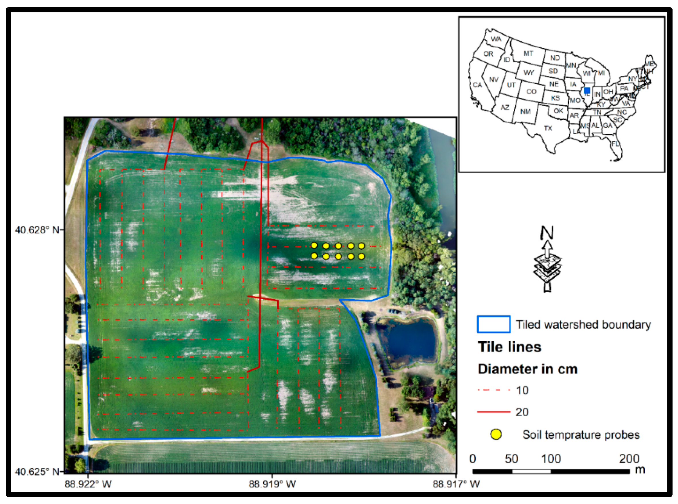
2. Study Site
3. Methods and Data
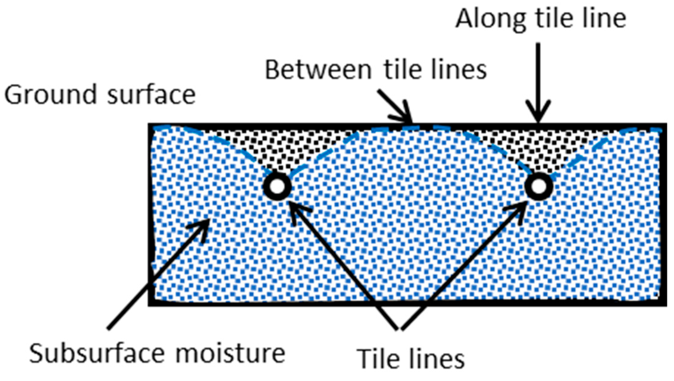
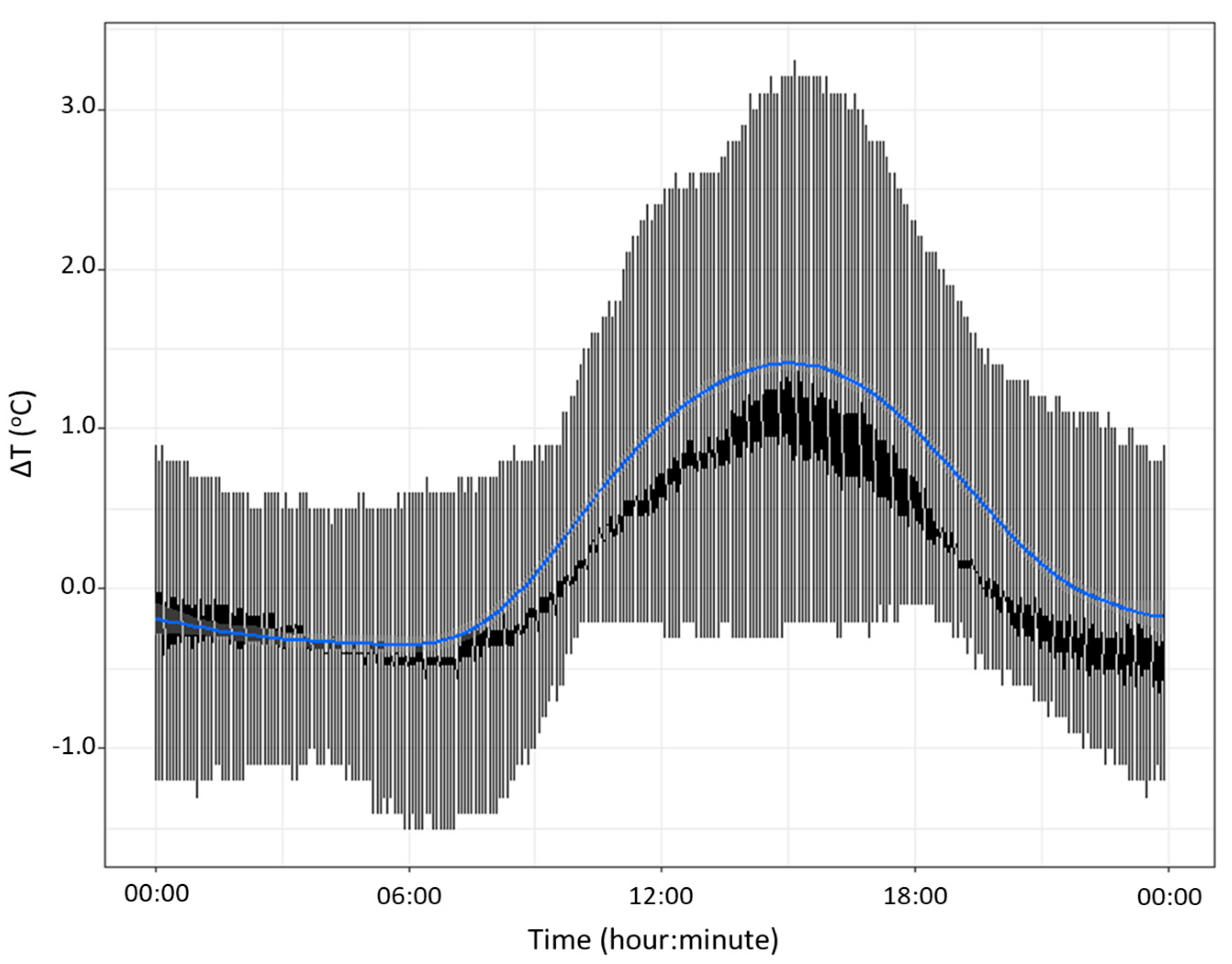
3.1. In-Situ Soil Temperature
3.2. Sensors
Thermal and Optical Sensors
3.3. UAS Flight Planning
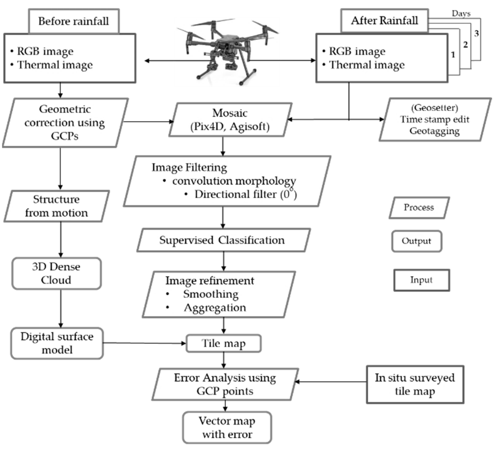
3.4. Data Processing and Analysis
3.4.1. Visible Image
3.4.2. Thermal Image
3.4.3. Data Analysis
- D = Euclidean distance
- i = the ith class
- x = n-dimensional data (where n is the number of bands)
- mi = mean vector of the class i
4. Results
4.1. In-Situ Soil Temperature
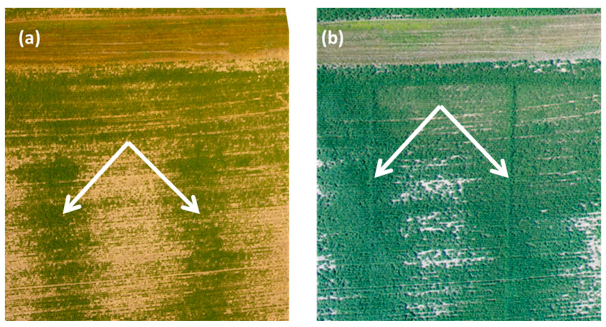
4.2. UAS Optical Imagery
4.3. Digital Surface Model (DSM)
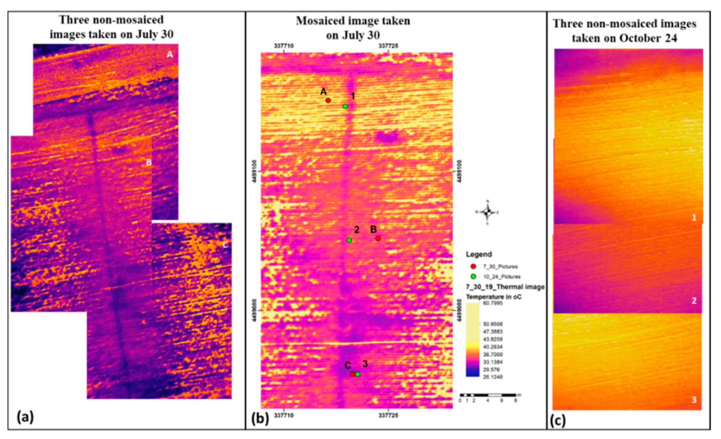
4.4. Radiometric Thermal Imagery
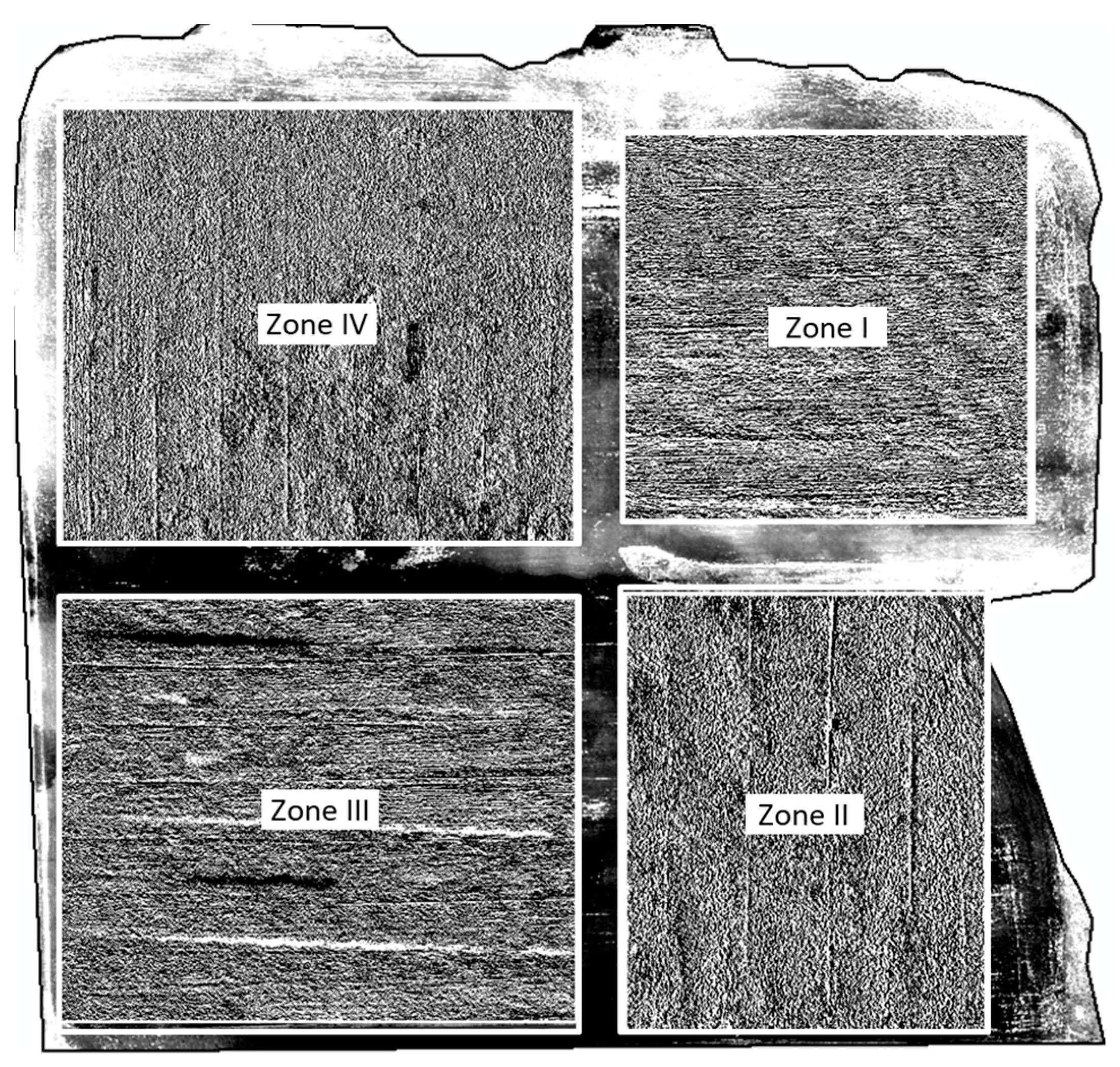
4.5. Image Processing
5. Discussion
6. Conclusions
Author Contributions
Funding
Institutional Review Board Statement
Informed Consent Statement
Data Availability Statement
Acknowledgments
Conflicts of Interest
References
- Van Metre, P.C.; Mahler, B.; Carlisle, D.; Coles, J.F. The Midwest Stream Quality Assessment—Influences of Human Activities on Streams; U.S. Geological Survey Fact Sheet 2017–3087: Reston, VA, USA, 2018.
- Naz, B.S.; Ale, S.; Bowling, L.C. Detecting subsurface drainage systems and estimating drain spacing in intensively managed agricultural landscapes. Agric. Water Manag. 2009, 96, 627–637. [Google Scholar] [CrossRef]
- Yannopoulos, S.I.; Grismer, M.E.; Bali, K.M.; Angelakis, A.N. Evolution of the Materials and Methods Used for Subsurface Drainage of Agricultural Lands from Antiquity to the Present. Water 2020, 12, 1767. [Google Scholar] [CrossRef]
- Kalita, P.; Cooke, R.; Anderson, S.; Hirschi, M.; Mitchell, J. Subsurface Drainage and Water Quality: The Illinois Experience. Trans ASABE 2007, 50, 1651–1656. [Google Scholar] [CrossRef]
- Valipour, M.; Krasilnikof, J.; Yannopoulos, S.; Kumar, R.; Deng, J.; Roccaro, P.; Mays, L.; Grismer, M.E.; Angelakis, A.N. The Evolution of Agricultural Drainage from the Earliest Times to the Present. Sustainability 2020, 12, 416. [Google Scholar] [CrossRef]
- Fausey, N.R.; Brown, L.C.; Belcher, H.W.; Kanwar, R.S. Drainage and Water Quality in Great Lakes and Cornbelt States. J. Irrig. Drain Eng. 1995, 121, 283–288. [Google Scholar] [CrossRef]
- Fausey, N.R. Drainage Management for Humid Regions. Int. J. Agric. Eng. 2005, 14, 209–214. [Google Scholar]
- Sugg, Z. Assessing US Farm Drainage: Can GIS Lead to Better Estimates of Subsurface Drainage Extent; World Resources Institute: Washington, DC, USA, 2007. [Google Scholar]
- Beauchamp, K.H. Chapter 2: A History of Drainage and Drainage Methods. In Farm Drainage in the United States: History, Status, and Prospects; Pavelis, G.A., Ed. Miscellaneous Publication No. 1455; Economic Research Service: Washington, DC, USA, 1987; Volume 186, pp. 13–29. [Google Scholar]
- Stillman, J.S.; Haws, N.W.; Govindaraju, R.S.; Rao, P.S.C. A semi-analytical model for transient flow to a subsurface tile drain. J. Hydrol. 2006, 317, 49–62. [Google Scholar] [CrossRef]
- Kornecki, T.S.; Fouss, J.L. Quantifying soil trafficability improvements provided by subsurface drainage for field crop operations in Louisiana. Appl. Eng. Agric. 2001, 17, 777–781. [Google Scholar] [CrossRef]
- Skaggs, R.W.; Brevé, M.A.; Gilliam, J.W. Hydrologic and water quality impacts of agricultural drainage. Crit. Rev. Environ. Sci. Technol. 1994, 24, 1–32. [Google Scholar] [CrossRef]
- Gilliam, J.W.; Baker, J.L.; Reddy, K.R. Chapter 24. Water Quality Effects of Drainage in Humid Regions. In Agricultural Drainage; Skaggs, R.W., van Schilfgaarde, J., Eds.; American Society of Agronomy: Madison, WI, USA, 1999; Volume Agronomy Monograph No. 38; pp. 801–830. [Google Scholar]
- Gardner, W.; Drendel, M.; McDonald, G. Effects of subsurface drainage, cultivation, and stubble retention on soil porosity and crop growth in a high rainfall area. Aust. J. Exp. Agric. 1994, 34, 411–418. [Google Scholar] [CrossRef]
- Williams, M.; King, K.; Fausey, N.R. Drainage water management effects on tile discharge and water quality. Agric. Water Manag. 2015, 148, 43–51. [Google Scholar] [CrossRef]
- Gökkaya, K.; Budhathoki, M.; Christopher, S.F.; Hanrahan, B.R.; Tank, J.L. Subsurface tile drained area detection using GIS and remote sensing in an agricultural watershed. Ecol. Eng. 2017, 108, 370–379. [Google Scholar] [CrossRef]
- Allred, B.J.; Redman, J.D. Location of Agricultural Drainage Pipes and Assessment of Agricultural Drainage Pipe Conditions Using Ground Penetrating Radar. J. Environ. Eng. Geophys. 2010, 15, 119–134. [Google Scholar] [CrossRef]
- Allred, B.; Eash, N.; Freeland, R.; Martinez, L.; Wishart, D. Effective and efficient agricultural drainage pipe mapping with UAS thermal infrared imagery: A case study. Agric. Water Manag. 2018, 197, 132–137. [Google Scholar] [CrossRef]
- Chow, T.L.; Rees, H.W. Identification of subsurface drain locations with ground-penetrating radar. Can. J. Soil Sci. 1989, 69, 223–234. [Google Scholar] [CrossRef]
- Lane, A.L.; Hedley, C.B.; McColl, S.T. Ground penetrating radar: The pros and cons of identifying physical features in alluvial soils. In Science and Policy: Nutrient Management Challenges for the Next Generation; Currie, L.D., Hedley, M.J., Eds.; Fertilizer and Lime Research Centre, Massey University: Palmerston North, New Zealand, 2017; Volume Occasional Report No. 30; p. 12. Available online: http://flrc.massey.ac.nz/publications.html (accessed on 1 November 2019).
- Naz, B.S.; Bowling, L.C. Automated Identification of Tile Lines from Remotely Sensed Data. Trans. ASABE 2008, 51, 1937–1950. [Google Scholar] [CrossRef]
- Seyoum, W.M. Characterizing water storage trends and regional climate influence using GRACE observation and satellite altimetry data in the Upper Blue Nile River Basin. J. Hydrol. 2018, 566, 274–284. [Google Scholar] [CrossRef]
- Seyoum, W.M.; Milewski, A.M.; Durham, M.C. Understanding the relative impacts of natural processes and human activities on the hydrology of the Central Rift Valley lakes, East Africa. Hydrol. Process 2015, 29, 4312–4324. [Google Scholar] [CrossRef]
- Seyoum, W.M.; Milewski, A.M. Improved methods for estimating local terrestrial water dynamics from GRACE in the Northern High Plains. Adv. Water Resour. 2017, 110, 279–290. [Google Scholar] [CrossRef]
- Seyoum, M.W.; Kwon, D.; Milewski, M.A. Downscaling GRACE TWSA Data into High-Resolution Groundwater Level Anomaly Using Machine Learning-Based Models in a Glacial Aquifer System. Remote Sens. 2019, 11, 824. [Google Scholar] [CrossRef]
- Zhang, C.; Kovacs, J.M. The application of small unmanned aerial systems for precision agriculture: A review. Precis. Agric. 2012, 13, 693–712. [Google Scholar] [CrossRef]
- Jeziorska, J. UAS for Wetland Mapping and Hydrological Modeling. Remote Sens. 2019, 11, 1997. [Google Scholar] [CrossRef]
- Tmušić, G.; Manfreda, S.; Aasen, H.; James, M.R.; Gonçalves, G.; Ben-Dor, E.; Brook, A.; Polinova, M.; Arranz, J.J.; Mészáros, J.; et al. Current Practices in UAS-based Environmental Monitoring. Remote Sens. 2020, 12, 1001. [Google Scholar] [CrossRef]
- Woo, D.K.; Song, H.; Kumar, P. Mapping subsurface tile drainage systems with thermal images. Agric. Water Manag. 2019, 218, 94–101. [Google Scholar] [CrossRef]
- Guan, X.; Huang, J.; Guo, N.; Bi, J.; Wang, G. Variability of soil moisture and its relationship with surface albedo and soil thermal parameters over the Loess Plateau. Adv. Atmos. Sci. 2009, 26, 692–700. [Google Scholar] [CrossRef]
- Rickels, E.S.; Stumpf, A.J.; Malone, D.H.; Shields, W.E. Surficial geology of the Saybrook 7.5-minute Quadrangle, Mclean County, Illinois, USA. J. Maps 2017, 13, 191–195. [Google Scholar] [CrossRef]
- Beekmans, C.; Schneider, J.; Läbe, T.; Lennefer, M.; Stachniss, C.; Simmer, C. Cloud photogrammetry with dense stereo for fisheye cameras. Atmos. Chem. Phys. 2016, 16, 14231–14248. [Google Scholar] [CrossRef]
- Roosevelt, C.H. Mapping site-level microtopography with Real- Time Kinematic Global Navigation Satellite Systems (RTK GNSS) and Unmanned Aerial Vehicle Photogrammetry (UAVP). Open Archaeol. 2014, 1, 29–53. [Google Scholar] [CrossRef]
- Agisoft LLC Agisoft Metashape 1.5.4; 2019. Available online: https://www.agisoft.com/ (accessed on 6 October 2020).
- Rumpler, M.; Tscharf, A.; Mostegel, C.; Daftry, S.; Hoppe, C.; Prettenthaler, R.; Fraundorfer, F.; Mayer, G.; Bischof, H. Evaluations on multi-scale camera networks for precise and geo-accurate reconstructions from aerial and terrestrial images with user guidance. Comput. Vision Image Underst. 2017, 157, 255–273. [Google Scholar] [CrossRef]
- Schmidt, F. GeoSetter, Version 3.5.3: Freeware Tool for Showing and Changing Metadata of Image Files. 2019. Available online: https://geosetter.de/en/main-en/ (accessed on 11 October 2020).
- Harris Geospatial Solutions, I. ENVI 5.5.1 (API version 3.3). 2018. Available online: https://www.l3harrisgeospatial.com/ (accessed on 12 October 2020).
- Putzig, N.E. Thermal inertia and surface heterogeneity on Mars. Ph.D Thesis, Colorado School of Mines, Golden, CO, USA, 2006. [Google Scholar]
- Haruna, S.I.; Anderson, S.H.; Nkongolo, N.V.; Reinbott, T.; Zaibon, S. Soil Thermal Properties Influenced by Perennial Biofuel and Cover Crop Management. Soil Sci. Soc. Am. J. 2017, 81, 1147–1156. [Google Scholar] [CrossRef]


| Parameter | FLIR Vue Pro R | DJI FC 6510 ZENMUSE X4S SPECS | DJI FC330 Phantom 4 Quadcopter |
|---|---|---|---|
| Spectral Range | 7.5–13.5 µm | 380–740 nm | 380–740 nm |
| Frame Rate | 30HZ | 14 frames per second | 30 frames per second |
| Data Format | Radiometric jpeg | DNG, JPEG, DNG+JPEG | JPEG, DNG RAW |
| Sensor Resolution | 640 × 512 | 16:9 (5472 × 3078), 4:3 (4864 × 3648) | 12 MP (4000 × 3000) |
| FOV | 45° × 35° | 84° | 94° |
| Thermal Sensitivity (NETD) | 0.02°C | N/A | N/A |
| Focal length (mm) | 13 | 24 | 20 |
| Weight (g) | 92–113 | 253 | 190 |
| Type of Camera | Flight Date | Flight Started | Flight Ended | Weather Condition (Max T. °C/Min T. °C) | Flight Altitude ABGL (m) | No. of Images Collected |
|---|---|---|---|---|---|---|
| FLIR Vue Pro R 640 | 22 July 2019 | 17:20:22 | 18:03:30 | 27/15 °C, partly cloudy, 24.4 mm rain on 5/7/2019 | 45 | 733 |
| 29 July 2019 | 16:51:40 | 17:27:14 | 31/18 °C, cloudy, 2.3 mm of rain on 27/7/2019 | 45 | 645 | |
| 30 July 2019 | 16:04:02 | 16:43:28 | 29/20 °C cloudy, 16.8 mm of rainfall the night before | 45 | 750 | |
| 24 October 2019 | 17:05:24 | 17:50:34 | 13/5 °C, Cloudy, 3.6 mm rain on 21/10 | 45 | 628 | |
| DJI FC 6510 ZENMUSE X4S | 6 August 2019 | 17:04:14 | 17:30:14 | 18/19 °C, Partly cloudy, 6.9 mm rainfall in the morning | 100 | 348 |
| 24 October 2019 | 15:15:00 | 15:30:00 | 13/5, Cloudy, 3.6 mm rain on 21/10 | 100 | 356 | |
| DJI FC330 phantom 4 Quadcopter | 15 July 2019 | 15:49:02 | 16:02:02 | 30/19 °C, windy and cloudy | 60 | 325 |
| Statistical Parameter | Date Collected | ||
|---|---|---|---|
| 22/7/2019 | 29/7/2019 | 30/7/2019 | |
| Min. Temperature | 15.01 | 20.82 | 15.03 |
| 1st Quartile | 29.17 | 32.41 | 32.69 |
| Median | 31.18 | 33.9 | 34.59 |
| Mean | 31.43 | 34.66 | 36.06 |
| 3rd Quartile | 33.41 | 36.18 | 38.27 |
| Max Temperature | 49.95 | 59.02 | 63.94 |
| IQR (interquartile Range) | 4.83 | 7.27 | 9.46 |
Publisher’s Note: MDPI stays neutral with regard to jurisdictional claims in published maps and institutional affiliations. |
© 2020 by the authors. Licensee MDPI, Basel, Switzerland. This article is an open access article distributed under the terms and conditions of the Creative Commons Attribution (CC BY) license (http://creativecommons.org/licenses/by/4.0/).
Share and Cite
Tilahun, T.; Seyoum, W.M. High-Resolution Mapping of Tile Drainage in Agricultural Fields Using Unmanned Aerial System (UAS)-Based Radiometric Thermal and Optical Sensors. Hydrology 2021, 8, 2. https://doi.org/10.3390/hydrology8010002
Tilahun T, Seyoum WM. High-Resolution Mapping of Tile Drainage in Agricultural Fields Using Unmanned Aerial System (UAS)-Based Radiometric Thermal and Optical Sensors. Hydrology. 2021; 8(1):2. https://doi.org/10.3390/hydrology8010002
Chicago/Turabian StyleTilahun, Tewodros, and Wondwosen M. Seyoum. 2021. "High-Resolution Mapping of Tile Drainage in Agricultural Fields Using Unmanned Aerial System (UAS)-Based Radiometric Thermal and Optical Sensors" Hydrology 8, no. 1: 2. https://doi.org/10.3390/hydrology8010002
APA StyleTilahun, T., & Seyoum, W. M. (2021). High-Resolution Mapping of Tile Drainage in Agricultural Fields Using Unmanned Aerial System (UAS)-Based Radiometric Thermal and Optical Sensors. Hydrology, 8(1), 2. https://doi.org/10.3390/hydrology8010002