Numerical Simulation of Flow in Parshall Flume Using Selected Nonlinear Turbulence Models

Abstract

This study uses a computational fluid dynamics (CFD) approach to simulate flows in Parshall flumes, which are used to measure flowrates in channels. The numerical results are compared with the experimental data, which show that choosing the right turbulence model, e.g., $v^2-f$ and LC, is the key element in accurately simulating Parshall flumes. The Standard Error of Estimate (SEE) values were very low, i.e., 0.76% and 1.00%, respectively, for the two models mentioned above. The Parshall flume used for this experiment is a good example of a hydraulic structure for which the design can be more improved by implementing a CFD approach compared with a laboratory (physical) modeling approach, which is often costly and time-consuming.

1. Introduction

Data from downscaled physical models of different hydraulic structures, such as dams, weirs, etc., were, in the past, the main resource for predicting the consequences of extreme damage. In recent years, with advancements in computing facilities and numerical modeling methods, numerical simulations have become a powerful and popular approach in the design of hydraulic structures [1].

There are various reasons, such as irrigation and quality control, for the importance of measuring the flowrate in an open channel, and this has led different individuals to come up with various ideas and designs for discharge measurement devices. One of the most popular devices is the Parshall flume, a modification of the Venturi flume, developed by Ralph L. Parshall in the 1930s. The major difference between this flume and the Venturi flume is the drop that was introduced in the throat’s bed elevation. This design, with a negative bed slope starting at the beginning of the throat section, helps fluid gain speed and, shortly before exiting the throat, a relatively gentle positive slope reduces the speed of the fluid at the exit of the throat section. The relationship between the head at two locations within the flume, i.e., the throat and upstream, provides a value for the flowrate in the open channel [2].

The available sizes for Parshall flumes are limited, and in addition, within this limited range, manufacturers tend to contravene the original specifications provided by Parshall as the inventor. To create a custom-size Parshall flume, many experiments have to be undertaken by the manufacturers to ensure the accuracy of the flowrate within the device. It is costly and time-consuming to run the necessary laboratory experiments for a new size, and using a Computational Fluid Dynamics (CFD) model can significantly accelerate the process [3].

Computer simulations are an essential tool in the design and optimization of hydraulic structures at present, and recent advancements in computing hardware now also allow researchers and engineers to solve previously impossible equations. Fluid motion is one of the most complicated engineering phenomena, and a particular approach to solving a fluid’s governing equations depends on the hardware limitations and available time. Various turbulence models are available within different computational fluid dynamics simulation software, and obtaining the best possible hydraulic structural design is possible through the use of CFD simulations. It is important to choose the best model with respect to the cost of calculations and accuracy. Therefore, in this paper, three nonlinear turbulence models from the RANS family were chosen to simulate the flow of water in a 3-inch Parshall flume, and the data from the simulations are compared with the experimental results from a study conducted by Dursun [4].

The study by Wright et al. [5] on the Parshall flume rating curve revealed that calibration for low-discharge flows for the Parshall flume had not been carried out; therefore, there was a bias in the results provided by Parshall himself for the proposed relationship. In their paper, they tried to provide a solution to this flaw, and so a numerical model was established to address the effect of the viscosity of the fluid on the depth discharge relationship. Experiments on a variety of flumes that carried only 15% of the recommended discharge revealed that the flowrate was overpredicted by 25%. The proposed numerical model for the low discharges provided a good match with the experimental data obtained in the laboratory.

Khosronejad et al. [6] implemented a Large Eddy Simulation (LES) model to determine the accuracy of Parshall flume discharge results in comparison with the experimental data. Their study was conducted on two Parshall flumes that were placed in a parallel arrangement, and the results were taken either from the flow passing through an individual flume when the other flume was closed or with the flow passing through both flumes at the same time. In addition to the flow measurement device used in this experiment, a dye dilution approach was also implemented to determine flow rates in the field. The difference between the standard rating curve value and the modeled value according to their study was, at maximum, 10%, while the discharge was at the lower flow rate for all three different scenarios, i.e., flows passing through flumes individually or in parallel, and was a minimum of 1.3% when the discharge was between 1.13 and 1.7 $m^3/s$ in the parallel flow case. It was concluded that a Parshall flume could provide more accurate results when operated at higher flowrates.

Davis and Deutsch [7] conducted studies on Parshall flumes with nonstandard positioning: the slope of the stream, the upstream velocity profile, and alterations in Parshall flume geometry were investigated in this research. Due to the implementation of SOFA-LUMP, a 3D finite-difference code, the simulated flowrates were accurate enough and the computational cost was under the expected budget. A downside of this study was the neglect of the viscosity effects in the numerical model; however, the numerical results were close to the experimental findings. The authors concluded that the proposed numerical model could be used as a guideline to determine the results for nonstandard Parshall flumes, and that the numerical model was the best substitute for laboratory experiments or field installations for accurate results.

Sun et al. [8] investigated the flow in a flume with symmetrical curve obstructions on the flume’s sides, and the results revealed that there was an incremental velocity increase within the throat section and a sudden flowrate decrease due to the introduction of a submerged flow condition at the end of that section. A comparison of water levels between the laboratory experiments and the numerical simulations showed a 4.7% error value, which was described as a good agreement. Due to its high accuracy and lower head loss, the proposed curved flume was believed to be an ideal choice for implementation from mild sloped flows to flat ones, e.g., for agriculture and irrigation systems.

Savage et al. [9] tackled the common problem of nonstandard entrance wingwalls in Parshall flumes, which is often neglected. To obtain proper results, it is important to know the best upstream location to measure the head for the flume. It was shown that CFD is a better tool, providing more accurate data compared to the costly physical “build and test” method. This paper introduced a correction factor for a range of different sizes (2–8 ft) of Parshall flumes, to adjust their results, and the implementation of this study for a nonstandard Parshall flume with a free-flow condition increased the accuracy of the discharge results from a 60% error to just +/−5%.

In a study by Heyrani et al. [10], the data from seven different turbulence models were compared with the experimental results from Dursun [4]. In the paper, it was concluded that, among the Reynolds-average Navier–Stokes (RANS), Large Eddy Simulation (LES), and Detached Eddy Simulation (DES) models, the best performance was achieved by the $k-\epsilon$ model from the RANS family, while the Dynamic K LES model was in second place. The water level results from the CFD simulations provided an error of less than 1.93%–2.08% compared to the experimental findings and were reasonably acceptable for further implementation. Although several turbulence models were examined in the study, some important ones remained unused, which are the subject of the present paper.

The objective of this paper is to extend the study by Heyrani et al. (2021) with more sophisticated, and potentially more accurate, turbulence models in order to develop highly accurate yet efficient modeling approaches for Parshall flumes. Two nonlinear $k-\epsilon$ models, which have proved to be highly accurate in certain fluid problems, are considered. In addition, the $v^2-f$ model, which is a compromise between the computational efficiency of two-equation models and the accuracy of the Reynolds Stress Models (RSM), is also considered in this study.

This paper is organized as follows. Governing equations and description of turbulence models are provided in Section 2, and numerical details such as mesh, boundary, and initial conditions are then described in Section 3. Next, results and discussions are presented in Section 4, and some concluding results complete the study.

2. Methodology

2.1. Description of CFD Model

As one of the most reliable tools to analyze the behavior of fluids, Computational Fluid Dynamics (CFD) is capable of calculating a wide range of related parameters by taking advantage of the recent development of computer processors. The parameters that are accurately calculated by CFD include flow velocity, temperature and pressure.

CFD models are capable of providing solutions for the flow equations or describing the behavior of a fluid when it interacts with rigid boundaries or obstacles along its path. With respect to the conservation of mass, energy, and momentum, the Navier–Stokes system of equations is derived for viscous fluids [11].

As a reliable open-source solver for computational fluid dynamics models, OpenFOAM is implemented in this study to perform reliable simulations. This computing platform uses the Finite Volume Method (FVM) and includes many specific libraries developed in C++. It is an object-oriented toolbox that can simulate a wide range of flow problems, such as two-phase flows and free-surface flows, with a wide range of turbulence models. It also has the ability to numerically solve continuum mechanics problems [12].

Three nonlinear turbulence models are used to simulate the flow motion in this paper, i.e., the LC low-Reynold, SQ low-Reynold, and $v^2-f$ models, which are briefly discussed in the following section.

2.2. Governing Equations

A viscous incompressible fluid flow is governed by a set of general three-dimensional systems of equations called the Navier–Stokes system, which consists of momentum and continuity equations. The system is described as follows [13,14]:

$$\frac{\partial u}{\partial x}+\frac{\partial v}{\partial y}+\frac{\partial w}{\partial z}=0$$

(1)

Equation (1) is the continuity equation, followed by the three momentum equations (Equations (2)−(4)) for different directions, i.e., x, y, and z directions.

$$\frac{\partial u}{\partial t}+u\frac{\partial u}{\partial x}+v\frac{\partial u}{\partial y}+w\frac{\partial u}{\partial z}=-\frac{1}{\rho }\frac{\partial p}{\partial x}+\nu {𝛻}^{2}u$$

(2)

$$\frac{\partial v}{\partial t}+u\frac{\partial v}{\partial x}+v\frac{\partial v}{\partial y}+w\frac{\partial v}{\partial z}=-\frac{1}{\rho }\frac{\partial p}{\partial y}+\nu {𝛻}^{2}v$$

(3)

$$\frac{\partial w}{\partial t}+u\frac{\partial w}{\partial x}+v\frac{\partial w}{\partial y}+w\frac{\partial w}{\partial z}=-\frac{1}{\rho }\frac{\partial p}{\partial z}+\nu {𝛻}^{2}w-g$$

(4)

In the above equations, fluid density is denoted by $\rho$, the three spatial directions of velocity are represented by $u$, $v$, and $w$, $p$ denotes the total pressure, time is symbolized by $t$, and $g$ is the gravitational acceleration.

2.2.1. RANS

The Reynolds-Averaged Navier–Stokes Model is the dominant practical method for simulating the motion of a fluid. Other methods, such as Large Eddy Simulation (LES), are computationally more expensive and still impractical for engineering applications. The viscosity-related properties of the fluid are essentially used to estimate the impact of turbulence. The variation in the turbulent kinetic energy (k) is described by an equation for k.

A variety of turbulence models are available under this category, and the application of three non-linear approaches to form a comparison with the experimental data forms the main objective of this study.

v² − f Model

A modified version of the $k-\epsilon$ model, where k represents the turbulent kinetic energy and $\epsilon$ denotes the energy dissipation, is called the $v^2-f$ turbulence model, which consists of four equations to simulate the effect of turbulence to find a solution for fluid flow motion. It has two extra equations for velocity and relaxation factors, as well as the two general kinetic energy and dissipation equations. This model falls between the categories of the Reynolds Stress Models (RSM) and the original $k-\epsilon$ model. In order to evaluate eddy viscosity with this model, the new term $v^2$, which represents the velocity, is implemented instead of the term for kinetic energy. The governing equations of this model are as follows:

$$\frac{\partial k}{\partial t}+\frac{\partial k{u}_i}{\partial x_i}=P-\epsilon +\frac{\partial }{\partial x_j}(D{k}_{eff}\frac{\partial k}{\partial x_j})+S_k$$

(5)

$$\frac{\partial \epsilon }{\partial t}+\frac{\partial \epsilon u_i}{\partial x_i}=\frac{C_{\epsilon 1}^{\prime }P-C_{\epsilon 2}\epsilon }{T}\frac{\partial }{\partial x_j}(D{\epsilon }_{eff}\frac{\partial \epsilon }{\partial x_j})+S_{\epsilon }$$

(6)

$$\frac{\partial \overline{V^2}}{\partial t}+\frac{\partial \overline{V^2}{u}_i}{\partial x_i}=kf-6\overline{V^2}\frac{\epsilon }{k}\frac{\partial }{\partial x_j}(D{k}_{eff}\frac{\partial \overline{V^2}}{\partial x_j})+S_{\overline{V^2}}$$

(7)

$$f-L^2\frac{{\partial }^{2}f}{\partial x_i{}^2}=(C_1-1)\frac{\frac{2}{3}-\frac{\overline{V^2}}{k}}{T}+C_2\frac{P}{k}+(\frac{5\overline{V^2}/k}{T})+S_f$$

(8)

In the above equations, the length and time-scales for turbulence are denoted by $L$ and $T$, while $f$ represents the solution to the last equation. The elliptic operator is used by the $v^2-f$ model to calculate a similar term to the strain–pressure correlation term of the RSM. There are four different constant $C$ terms, i.e.,$C_1$, $C_2$, $C_{\epsilon 1}^{\prime }$, and $C_{\epsilon 2}$, which are considered the constants, and the four $S$ terms, i.e.,$S_k$, $S_{\epsilon }$, $S_{\overline{V^2}}$, and $S_f$, which are expected to be defined by the user as source terms. The reader is referred to [15] for further details and values of the coefficients.

Shih et al. (1998) Quadratic k − ε Model (SQ)

This model is derived from the direct implementation of a basic turbulence relationship. To propose a novel algebraic equation for the Reynolds stress, an essential turbulent relationship has been applied. Two limitations are defined based on their realizability and the theory of rapid distortion and, within the inertia sublayer, the coefficients of the model are regulated using simple flows, such as surface flow and homogenous shear flow.

Quadratic and cubic terms of average velocity in the model were proposed for Reynolds stresses. This is a short version of the general formula for mean velocity gradients and turbulent stresses [16]. The rapid distortion theory was used to determine the coefficients of the model’s constraints [17] of realizability [18].

The equations used to model the general turbulent shear flow are:

$${\rho }_{,t}+{\left(\rho U_j\right)}_{,j}=0$$

(9)

$${\left(\rho U_i\right)}_{,t}+{\left(\rho U_i{U}_j\right)}_{,j}=-P_{,i}+{\left[\mu \left(U_{i,j}+U_{j,i}-\frac{2}{3}{U}_{k,k}{\delta }_{ij}\right)-\rho \overline{u_i{u}_j}\right]}_{,j}$$

(10)

$${\left(\rho k\right)}_{,t}+{\left(\rho U_{i}k\right)}_{,i}={\left[\left(\mu +\frac{{\mu }_T}{{\sigma }_k}\right)k_{,j}\right]}_{,j}-\rho \overline{u_i{u}_j}{U}_{i,j}-\rho \epsilon$$

(11)

$${\left(\rho \epsilon \right)}_{,t}+{\left(\rho U_i\epsilon \right)}_{,i}={\left[\left(\mu +\frac{{\mu }_T}{{\sigma }_{\epsilon }}\right){\epsilon }_{,j}\right]}_{,j}+C_1{f}_1\rho S \epsilon -C_2{f}_2\rho \frac{{\epsilon }^2}{k+\sqrt{v\epsilon }}+C_3\frac{\mu {\mu }_T}{\rho }{S}_{,j}{S}_{,j}$$

(12)

where S in the above equation is defined as:

$$S=\sqrt{2S_{ij}{S}_{ij}} , S_{ij}=\frac{1}{2}\left(U_{i,j}+U_{j,i}\right)$$

The nonlinear model for the Reynolds stresses is:

$$\begin{array}{cc}\hfill -\rho \overline{u_i{u}_j}=-\frac{2}{3}\rho k& {\delta }_{ij}+{\mu }_T\left(U_{i,j}+U_{j,i}-\frac{2}{3}{U}_{k,k}{\delta }_{ij}\right)+A_3\frac{\rho k^3}{2{\epsilon }^2}\left(U_{k,i}{U}_{k,j}-U_{i,k}{U}_{j,k}\right)\hfill \\ & +A_5\frac{\rho k^4}{{\epsilon }^3}[U_{k,i}{U}_{k,p}{U}_{p,j}+U_{k,j}{U}_{k,p}{U}_{p,i}-\frac{2}{3}{\Pi }_3{\delta }_{ij}-\frac{1}{2}{U}_{l,l}\left(U_{i,k}{U}_{k,j}+U_{j,k}{U}_{k,i}-\frac{2}{3}{\Pi }_1{\delta }_{ij}\right)\hfill \\ & -\frac{1}{2}{U}_{l,l}\left(U_{k,i}{U}_{k,j}+U_{i,k}{U}_{j,k}-\frac{2}{3}{\Pi }_2{\delta }_{ij}\right)]\hfill \end{array}$$

(13)

$${\mathsf{\Pi }}_1=U_{i,j}{U}_{j,i} , {\mathsf{\Pi }}_2=U_{i,j}{U}_{i,j} , {\mathsf{\Pi }}_3=U_{i,k}{U}_{i,p}{U}_{p,k}$$

(14)

The equations used to obtain the coefficients value of ${\mu }_T$ and $A_3$ to $A_5$ are provided below:

$${\mu }_T=C_{\mu }{f}_{\mu }\rho \frac{k\left(k+\sqrt{v\epsilon }\right)}{\epsilon }, A_3=\frac{\sqrt{1-\frac{9}{2}{C}_{\mu }^2{\left(\frac{k{S}^{*}}{\epsilon }\right)}^{2 }} }{0.5+\frac{3}{2}\frac{k^2}{{\epsilon }^2}{\mathsf{\Omega }}^{*} S^{*}}, A_5=\frac{1.6 {\mu }_T}{\frac{p{k}^4}{{\epsilon }^3}\frac{7{\left(S^{*}\right)}^2+{\left({\mathsf{\Omega }}^{*}\right)}^2}{4} }$$

(15)

$$\begin{array}{c}{C}_{\mu }=\frac{1}{4+A_s{U}^{*}\frac{k}{\epsilon }} , C_1=\max \left\{0.43,\frac{\eta }{5+\eta }\right\}, C_2=1.9, C_3=1.0,\\ {\sigma }_k=1.0, {\sigma }_{\epsilon }=1.2, U^{*}=\sqrt{{\left(S^{*}\right)}^2+{\left({\mathsf{\Omega }}^{*}\right)}^2} , S^{*}=\sqrt{S_{ij}^{*}{S}_{ij}^{*}},\\ {\mathsf{\Omega }}^{*}=\sqrt{{\mathsf{\Omega }}_{ij}{\mathsf{\Omega }}_{ij}}, {\mathsf{\Omega }}_{ij}=\frac{1}{2}\left(U_{i,j}-U_{j,i}\right), S_{ij}^{*}=S_{ij}-\frac{1}{3}{S}_{kk}{\delta }_{ij},\\ \eta =\frac{S k}{\epsilon }, A_s=\sqrt{6}\cos \varphi , \varphi =\frac{1}{3}\arccos \left(\sqrt{6}{W}^{*}\right), W^{*}=\frac{S_{ij}^{*}{S}_{ji}^{*}{S}_{ki}^{*}}{{\left(S^{*}\right)}^3}\end{array}$$

(16)

The reader is referred to [19] for further details and values of the coefficients.

Lien (1996) Cubic Turbulence Model (LC)

A new version of an eddy-viscosity model for turbulent flows with high Reynolds numbers was derived in [15] by implementing a nonlinear association between the parameters of strain and Reynolds stresses. For low-Reynolds conditions, vorticity tensors were also included in this relationship to identify all the variations in the turbulence length scale close to the wall in an asymptotic manner.

Using series-expansion, a general and coordinate invariant formula for strains and stresses is possible, as follows:

$$\begin{array}{c}\frac{\overline{u_i^{\prime }{u}_j^{\prime }}}{k}=\frac{2}{3}{\delta }_{ij}-\frac{{\nu }_T}{k}{S}_{ij}+C_1\frac{{\nu }_T}{ϵ}\left[S_{ik}{S}_{kj}-\frac{1}{3}{\delta }_{ij}{S}_{kl}{S}_{kl}\right]+C_2\frac{{\nu }_T}{ϵ}\left[{\mathsf{\Omega }}_{ik}{S}_{kj}+{\mathsf{\Omega }}_{jk}{S}_{ki}\right]\\ +C_3\frac{{\nu }_T}{ϵ}\left[{\mathsf{\Omega }}_{ik}{\mathsf{\Omega }}_{jk}-\frac{1}{3}{\delta }_{ij}{\mathsf{\Omega }}_{kl}{\mathsf{\Omega }}_{kl}\right]+HOT\end{array}$$

(17)

where $C_{\mu }$ and $C_1$ to $C_3$, proposed by [20] and only applicable to high-Reynolds areas, are:

$$C_{\mu }=\frac{0.667}{A_1+S+0.9\mathsf{\Omega }}{|}_{A_1=1.25,}$$

(18)

$$C_1=\frac{3/4}{\left(1000+S^3\right)},C_2=\frac{15/4}{\left(1000+S^3\right)},C_3=\frac{19/4}{\left(1000+S^3\right)}$$

(19)

$$S_{ij}=\frac{\partial u_i}{\partial x_j}+\frac{\partial u_j}{\partial x_i},{\mathsf{\Omega }}_{ij}=\frac{\partial u_i}{\partial x_j}+\frac{\partial u_j}{\partial x_i},S=\frac{k}{ϵ}\sqrt{\frac{1}{2}{S}_{ij}{S}_{ij}},\mathsf{\Omega }=\frac{k}{ϵ}\sqrt{\frac{1}{2}{\mathsf{\Omega }}_{ij}{\mathsf{\Omega }}_{ij}}.$$

(20)

To inspect the consequence of streamline curvature, a cubic correction proposed by [21] is also used:

$$HOT=C_4\frac{{\nu }_{T}k}{{ϵ}^2}\left(S_{ki}{\mathsf{\Omega }}_{lj}+S_{kj}{\mathsf{\Omega }}_{li}\right)S_{kl}+C_5\frac{{\nu }_{T}k}{{ϵ}^2}\left(S_{kl}{S}_{kl}-{\mathsf{\Omega }}_{kl}{\mathsf{\Omega }}_{kl}\right)S_{ij}$$

(21)

where:

$$C_4=-10C_{\mu }^2\hspace{1em}{C}_5=-2C_{\mu }^2$$

(22)

The turbulent viscosity ${\nu }_T$ obtained from the $k-\epsilon$ modelling framework is described as:

$${\nu }_T=C_{\mu }\frac{k^2}{ϵ}$$

(23)

The reader is referred to [22] for further details and values of the coefficients.

2.3. Numerical Setup

The interFoam solver from the OpenFOAM family was chosen as the solver in this study, as it provides a blend of applications of the VoF method and the finite-volume method [10]. The Euler and Crank–Nicolson schemes were implemented as first- and second-order time schemes, respectively, to discretize the temporal term, while the Gauss linear method was applied for the gradient terms. The results from the two different temporal discretization schemes used in this study showed no significant differences, i.e., no significant improvement was observed when the second-order scheme was used. Therefore, using either method has no effect on the reduction in error. In other words, the time scheme has a negligible impact as the source of error. Within this solver, different schemes were used for different purposes, such as the corrected Gauss linear scheme for the Laplacian scheme and a linear scheme for the purpose of discretization of the interpolation terms.

As the initial condition, the inflows of the flume for different scenarios were constant, i.e., 10 l/s, 20 l/s, and 30 l/s. Similar to Heyrani et al. (2021), the flow passing through the walls was considered to be zero, and no dissipation or acceleration was initially defined in the model.

2.3.1. Boundary Conditions

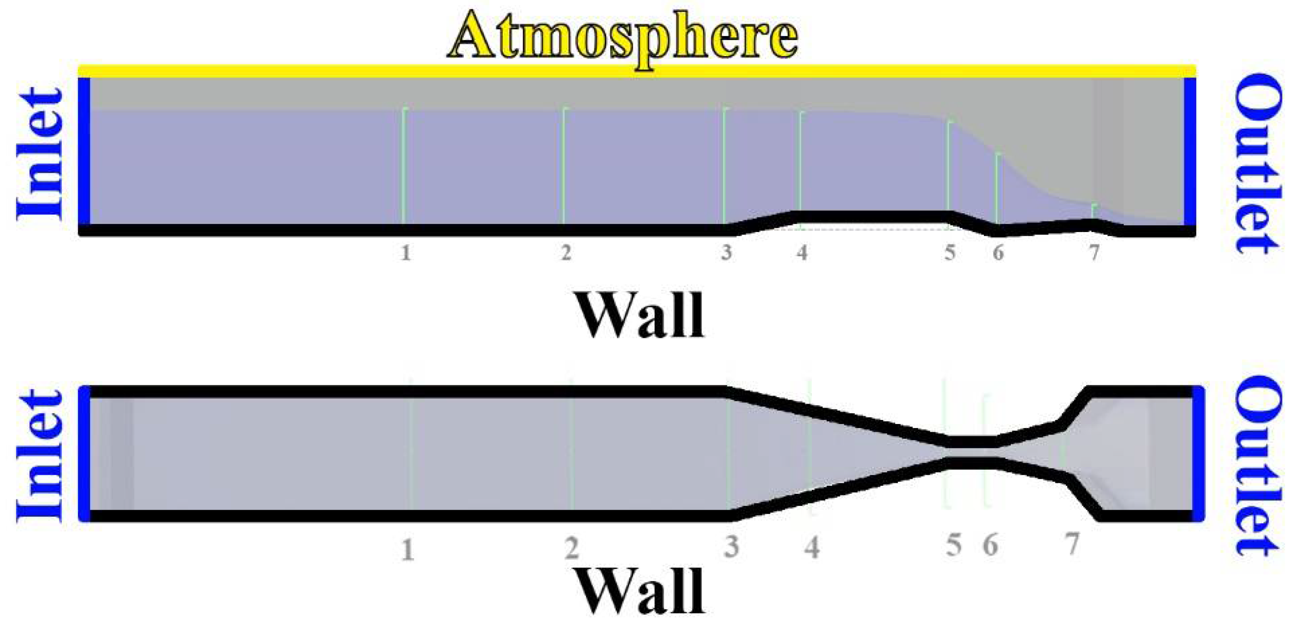
Figure 1 provides a schematic side and top view of the boundary condition considered in this simulation, where the flow enters and exits from one end to another while passing above the bed, which was defined as a wall. Over the flow is the atmosphere boundary, and the condition at the outlet is zero gradient. The volume of fluid method was implemented for the surface of the flow with regard to the zero-pressure state where the two fluids, i.e., liquid and air, meet.

2.3.2. Mesh Sensitivity Analysis

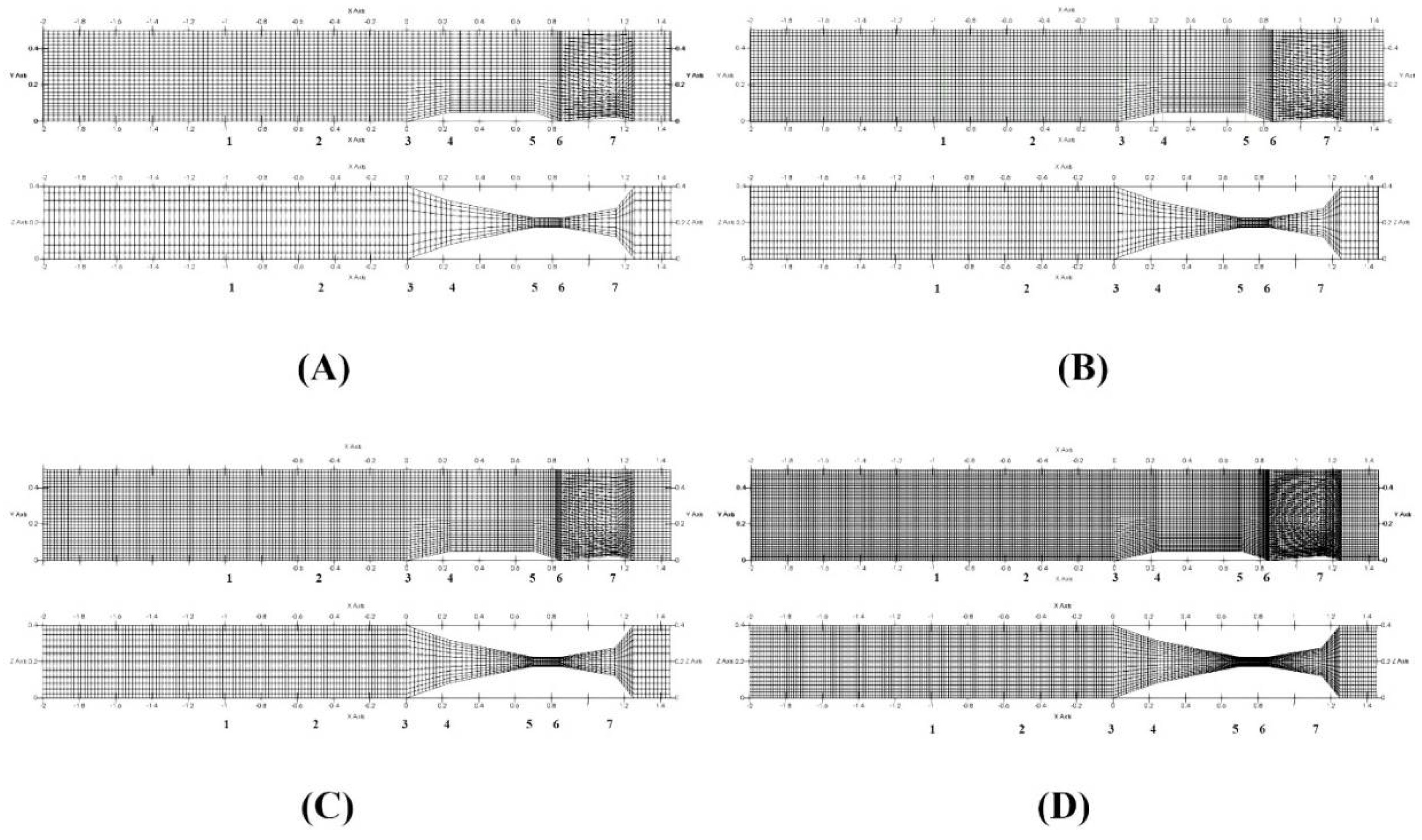
Implementing the right mesh size, i.e., the mesh closest to the optimum grid size, allows for the simulation to produce the results that are the closest to the actual data, i.e., experimental results, with an optimal computational cost. For the simulations in this study, a mesh sensitivity analysis was performed to determine the best grid size for the structured mesh that was used.

In this procedure, the refined mesh resolution was progressively increased until no further changes were obtained in the results. Figure 2 describe the four steps taken to find the optimum grid size in this study. This was started with 52,000 cells in total, progressing to 270,000 over three steps. The data quality resulting from the progression to the second step, i.e., from 52,000 to 75,000 cells, had significant changes, but on proceeding to 270,000, there were no significant changes recorded in the quality of the simulated data. Therefore, no further increase in the number of cells is recommended after 75,000.

2.4. Data

The trials that resulted in the experimental data were conducted by [4] at the hydraulic laboratory of Firat University in Elazig, Turkey. All experiments were completed in a flume with a rectangular shape and fixed dimensions of 0.4 m width, 5 m length, and 0.6m depth. Although the scope of Dursun’s study was the measurement of dissolved oxygen in the fluid before and after entering and exiting the flume, in the present study, only data for water levels were used. Flowrates of 10, 20, 30, and 40 l/s were chosen, which were measured with the help of an electromagnetic flow meter within a modifiable Parshall flume to obtain results that were sufficient to draw conclusions.

The time taken for the simulation to reach steady state was 50 seconds. With respect to the existing hardware that performed the simulation, i.e., Intel Xeon Processor E5-2683 v3 (35M Cache, 2.00 GHz) the total time taken to achieve steady-state, i.e., 50 seconds, was approximately 4 hours. Considering the total number of the cells used in all three simulations, i.e., 75000, the nonlinear model is not a costly model and could be considered in the future by other researchers.

The optimum number of time-steps to achieve a steady water level was found to be 150. The maximum height fluctuations were found to be less than 2% of the steady level height. ParaView was used as post-processing software to demonstrate the water levels and other properties of the flow passing through the flumes. To determine the height of a column of water as a representative segment in each selected cross-section, the line of intersection between two perpendicular planes passing through the column point was found. Then, using the value of the Y coordinate of each datapoint, the water level was determined.

3. Results

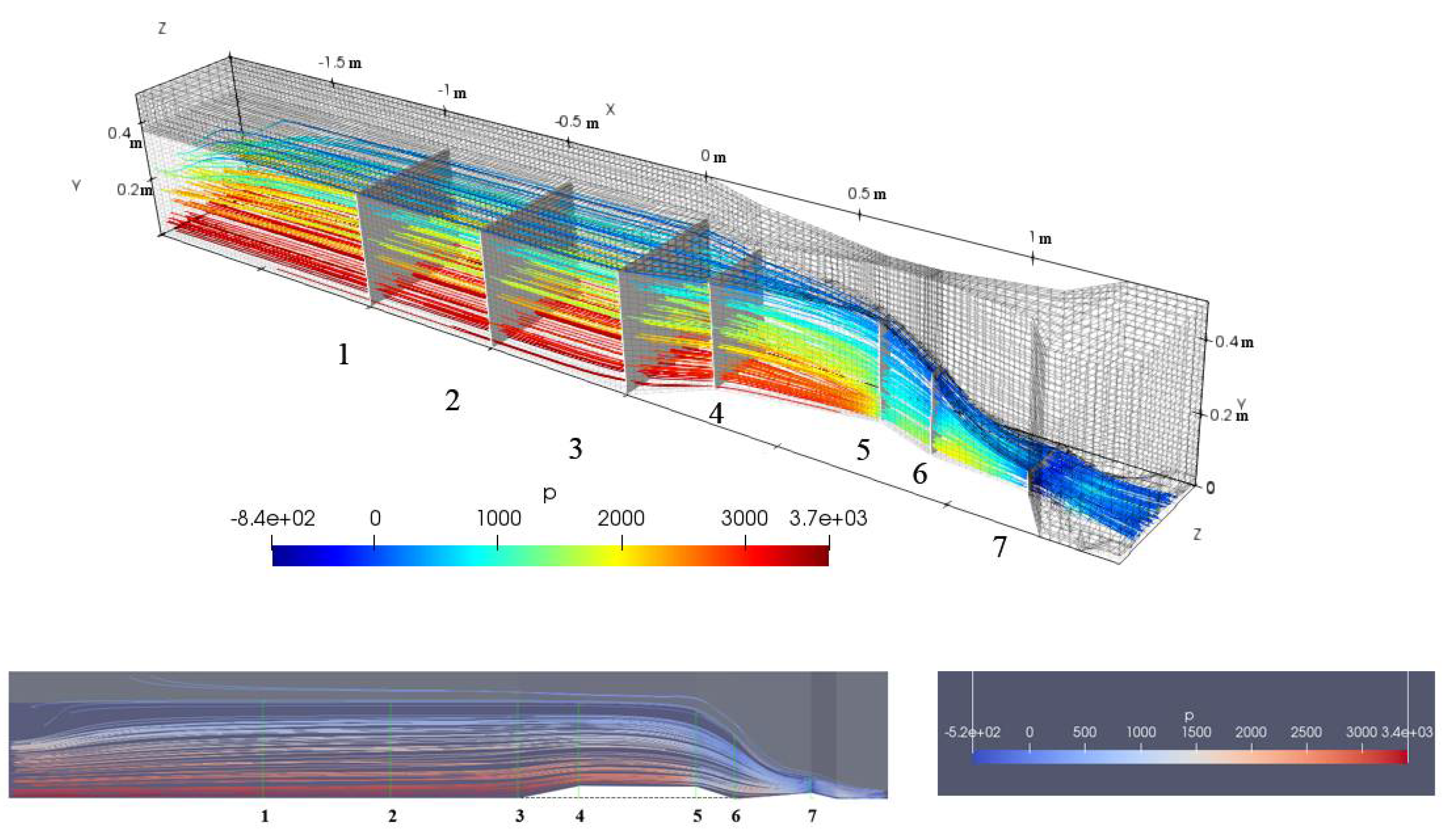
The water levels at different sections of the flume were measured for comparison with the experimental results obtained by Dursun (2016). Figure 3 illustrates the geometry and dimensions of the Parshall flume used in the simulation. Water enters the main channel, which has a width of 40 cm, i.e., cross-sections 1 and 2, and, with the help of wing walls, it gradually enters the throat section, which has a 5-cm wall-to-wall distance. The length of the throat, i.e., the distance between cross-sections 5 and 6, is 15 cm. Finally, the flow passes the divergence section, where the slope of the bed gradually becomes positive after cross-section 6.

As shown in Figure 3, seven locations were chosen along the x-axis to assess the water levels for this experiment. As, in the previous study by Heyrani et al. [10], the adjustment of the first sampling location was suggested to obtain more accurate results, cross-section number one was shifted forward, to where fewer fluctuations occur. The locations of the remaining cross-sections were selected as at the beginning of each transition in the flume, i.e., cross-sections 3 and 4 were where the convergence section starts and cross-section 5 was at the start of the throat section. The remaining cross-sections followed the same pattern.

The model was run with four different grid sizes to find the most suitable one, to obtain better-quality data. Among the different cell quantities tried in this study, i.e., 27,000, 52,000, 75,000, and 275,000, the results tended to remain the same with cell numbers of 52,000 and above.

The models were also run with three different flowrates, i.e., 10 l/s, 20 l/s and 30 l/s, and the smallest error was achieved for the 20 l/s discharge.

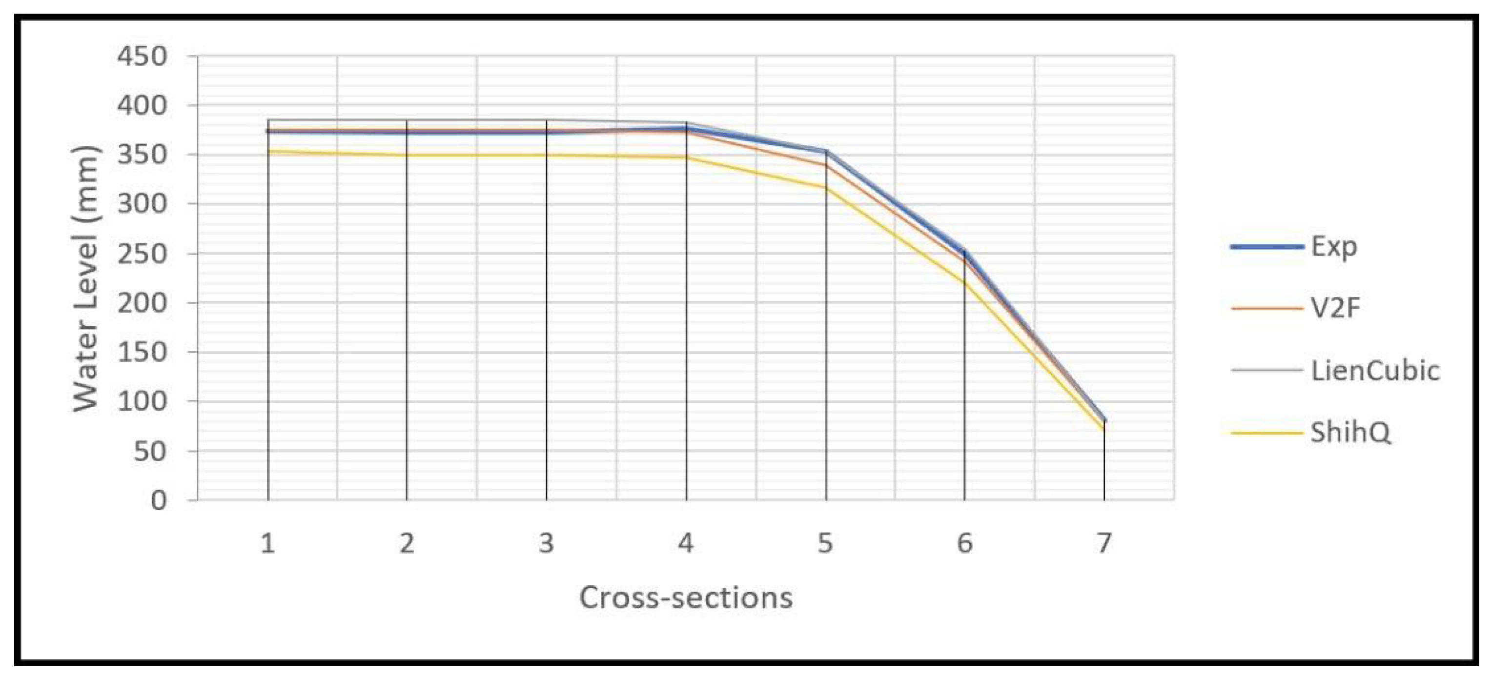
Figure 4 illustrates the water levels obtained using the three different turbulence models versus the experimental results from Dursun (2016). The performance of the nonlinear models was found to be more precise compared to the other turbulence models used by Heyrani et al. (2021). The error value derived with Equation (25) for the $v^2-f$ model, which was the lowest among the three, was 0.76%.

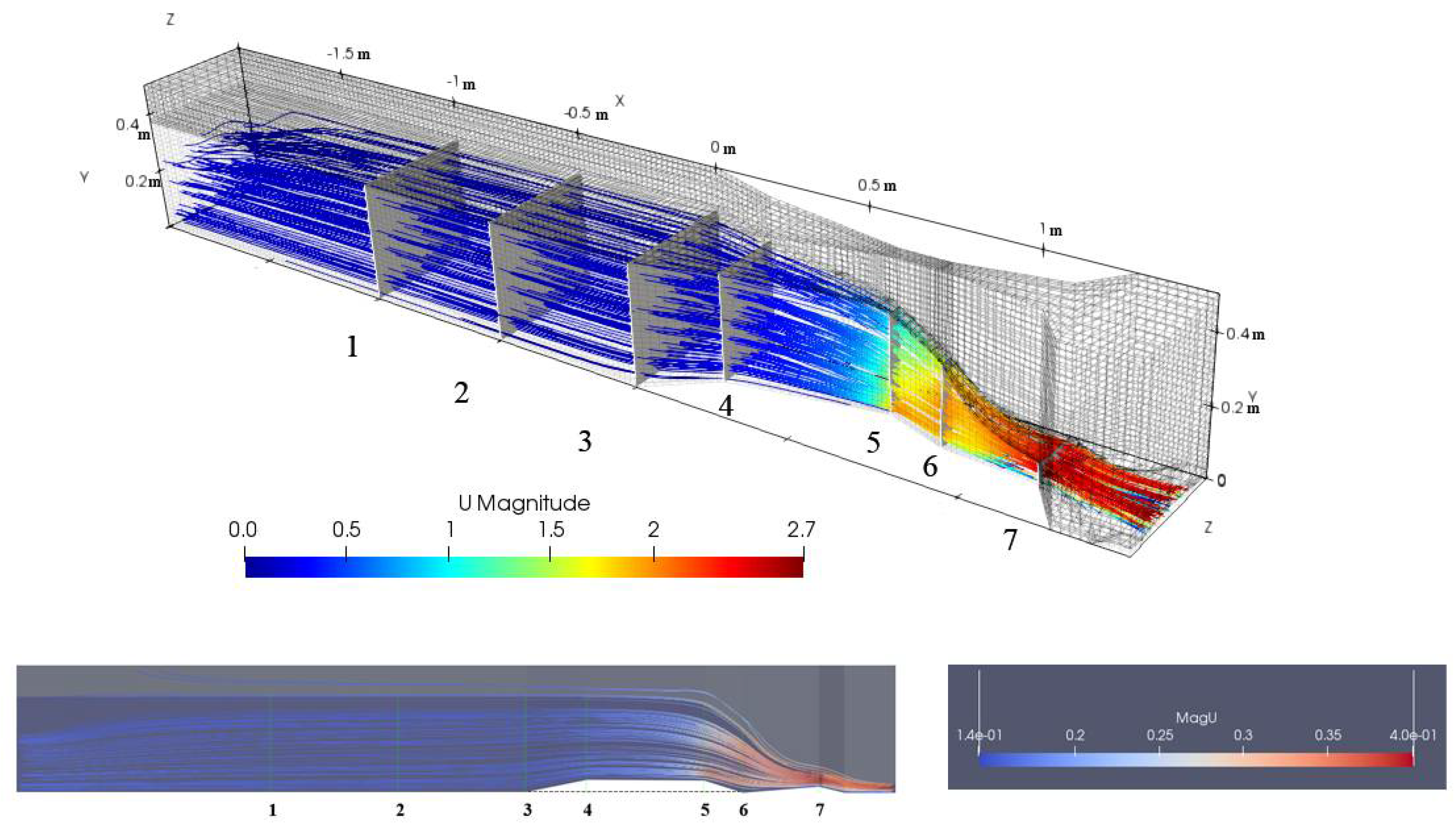
Figure 5 shows the velocity gradient of the flow passing through the flume. The contraction at the beginning of the throat, i.e., cross-section 5, forces the flow to gain velocity until it reaches its highest point at cross-section 7, where it experiences the maximum velocity downstream at the second diverging section. Parshall flume’s design leads to an increase in flow velocity at certain sections, while the flowrate remains constant.

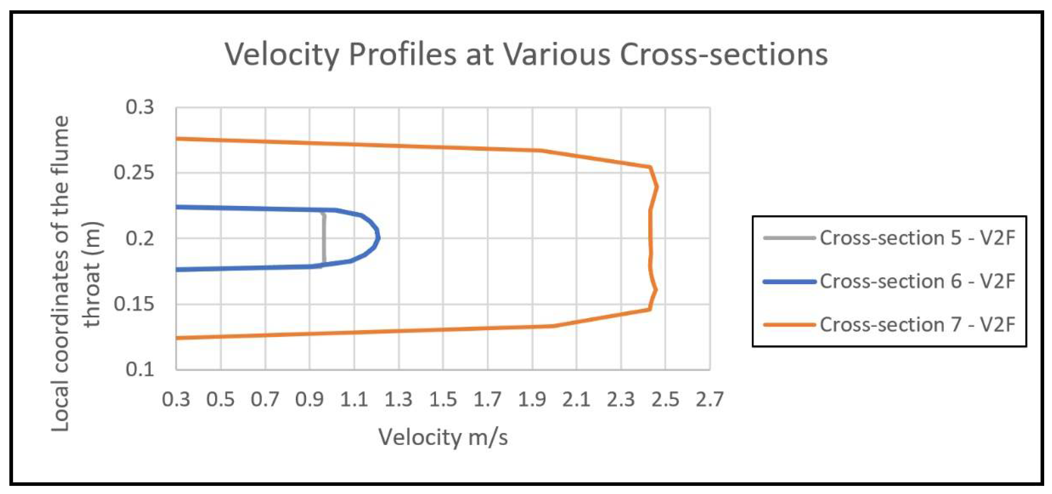
The velocity profiles at cross-sections 5, 6, and 7 are presented in Figure 6. As shown in Figure 5, the flow speed variation gradually increases along the flow path. At different cross-sections in Figure 6, the maximum speeds were 0.97, 1.21, and 2.45 m/s, respectively, from cross-sections 5 to 7. Due to the shape of the flume, the distribution of the velocity profiles was varied in shape, e.g., at cross-section 5 it was distributed evenly, but as the flow moves forward, the velocity concentration shifted toward the center of the cross-section. The diverging shape of section 7 is the reason that the velocity distribution was concentrated at the sides and not the center.

As illustrated in Figure 7, the flow’s pressure field gradient was the lowest when the flow achieved a higher speed from cross-sections 5 to 7. Due to the presence of the throat contraction, a higher pressure was present downstream over the entire flow up to the start of the throat section.

4. Discussion

Different methods of comparing of the water levels estimated from OpenFOAM versus the experimental results from the case study are illustrated in

Table 1. Error percentage calculated by Equation (24) of the estimated values for the three turbulence models across 7 cross-sections.

	Error Percentage
Cross-Sections	1	2	3	4	5	6	7
V2-F	0.29%	0.55%	0.79%	1.05%	3.92%	3.13%	2.83%
LienCubic(LC)	2.97%	3.23%	3.48%	1.60%	0.25%	2.10%	1.60%
ShihQ(SQ)	5.59%	6.42%	5.93%	7.95%	10.70%	11.57%	12.67%

and

Table 2. Average error, Standard Error of Estimate (SEE), Square of Correlation coefficient $R^2$ vs. experimental data.

Turbulence Model	Average Error %	SEE %	${\mathit{R}}^2$	$(1-{\mathit{R}}^2)\mathit{\%}$
V2F	1.79%	0.76%	0.9971	0.29 %
LienCubic(LC)	2.17%	1.00%	0.9985	0.15 %
ShihQ(SQ)	8.69%	3.09%	0.9959	0.41 %

. The relationships used to calculate the error values are as follows:

$$Error=\frac{\left|x_{exp}-x_{sim}\right|}{x_{exp}}$$

(24)

$$Standard Error of Estimate \left(SEE\right)=\sqrt{\frac{{{\displaystyle \sum }}_{i=1}^n{\left(x_{ex{p}_i}-x_{si{m}_i}\right)}^2}{n-2}}$$

(25)

$$R^2=\frac{{{\displaystyle \sum }}_{i=1}^n{\left(x_{ex{p}_i}-\overline{x_{exp}}\right)}^2}{{{\displaystyle \sum }}_{i=1}^n{\left(x_{si{m}_i}-\overline{x_{exp}}\right)}^2}$$

(26)

The Standard Error of Estimate (SEE) and the correlation coefficient (R) were calculated to estimate the errors of the simulation data. Table 1 and Table 2 shows the calculated error values.

Equation (24) was applied to each individual cross-section and returned a separate error value for each of them, while Equations (25) and (26) provided a single overall value for each dataset, i.e., data from the LC simulation or the $v^2-f$ model. To represent a single value for an error obtained by Equation (24), an average value was considered for all seven cross-sections.

In an overall analysis of the error percentages, for the first four cross-sections, the $v^2-f$ turbulence model provided the least amount of error, while the SQ model returned the highest amount of error for the same sections. Moving to the subsequent sections, $v^2-f$ lost its superiority over the LC turbulence model, where, for all three remaining cross-sections, the LC model provided the least amount of error. The SQ model in this study delivered unacceptable results compared to the other two, and as the average error percentages in Table 2 show, the $v^2-f$ model was higher than the rest.

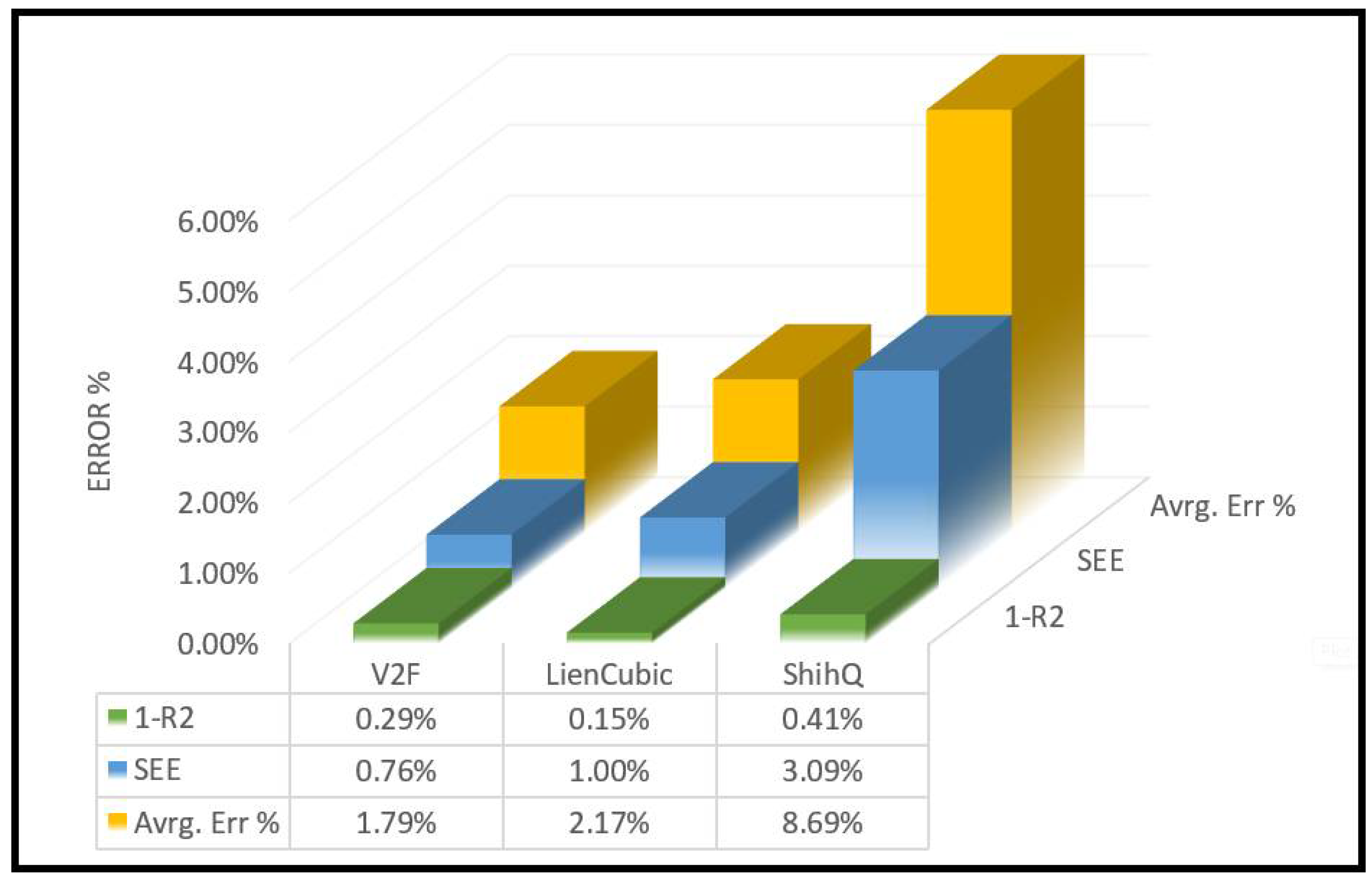
As described above, different methods were used to determine how far the simulation results were from the experimental ones. The standard square of estimate is one useful method for estimating the exactness of any prediction. The values produced by this method were 0.76% for the $v^2-f$ model, 1.00% for the LC model, and 3.09% for the SQ model. This is another proof of the accuracy of the $v^2-f$ model for this scenario. The correlation coefficient and the root mean square value are also counted as two other proofs of the superiority of the $v^2-f$ turbulence model.

4.1. SQ Model

The error values from this turbulence model’s estimates show higher error percentages than the different methods, and the overall performance of this model was the poorest among the three. As shown in Figure 8 and Figure 9, the average error values for the different cross-sections increased rapidly compared to the other two models. The maximum error value is recorded when the mean value of the error percentages for the seven different cross-sections is calculated.

4.2. LC Model

The correlation coefficient values that were closest to the experimental data were obtained from this model, i.e., 1-0.15%=0.9985 (99.85%), as shown in Figure 9. Additionally, the last three cross-sections tended to have the lowest error percentage values under the Lien Cubic model. This model produces error values that are almost identical to the $v^2-f$ model, but slightly higher. Compared to the SQ model, after the $v^2-f$ model, the data from the LC model are considered reliable.

4.3. ${\mathit{v}}^{\mathbf{2}}\mathbf{-}\mathit{f}$ Model

Of all the methods used to determine the error percentages of the estimated water levels, compared to the experimental one, this model provided the least error and was the most accurate. Aside from the lack of accuracy regarding the last three cross-sections, i.e., 5, 6, and 7, this model is the most recommended based on the results of this study.

5. Conclusions

The objective of this research was to study the reliability of numerical simulations of a Parshall flume using various nonlinear turbulence models. This is the first time that these state-of-the-art turbulence models have been employed to investigate the hydrodynamic performance of the Parshall flumes.

This study was specifically performed in alignment with the previous research conducted by Heyrani et al. [10]; however, the methods and turbulence models described here have been enhanced to provide more accurate results. Additionally, the recommendations offered in the other paper are implemented in this study where applicable, i.e., in the selection of locations for cross-section number 1. The following points are the main highlights of this research:

• The comparison of three nonlinear turbulence models, i.e., the LC, SQ, and $v^2-f$ models, reveals that the results obtained from these nonlinear models, except for the SQ model, lead to higher accuracy when compared with the experimental data, as shown in Table 1 and Table 2, where the mean error values over all seven cross-sections are 1.79% and 2.17% for the $v^2-f$ and LC models, respectively.
• The use of $v^2-f$ and LC models in this study is considered a significant improvement since, in the previous study by Heyrani et al. [10], with the similar initial criteria of the model parameters, none of the seven turbulence models from the three different families of RANS, LES and DES were able to provide the accuracy of the $v^2-f$ and LC results when compared to the experimental data, especially the $v^2-f$ model. However, these two non-linear turbulence models could be considered when the highest accuracy is demanded under similar conditions.
• The performance of the quadratic model in this simulation was not adequate and led to a high error percentage, well beyond the desired boundary. Hence, it is strongly recommended that, if the nonlinear model is chosen, the quadratic model is not used when dealing with Parshall flume modeling with similar specifications and flowrate value.
• The results strongly support the possibility of using CFD simulation as a reliable and cost-effective solution for a variety of different hydraulic projects. It was not only proven to be cost-effective compared to laboratory-scale simulations, but is also less time-consuming, depending on how powerful the computer system is.
• With respect to the enhancement of the Parshall flume design, implementing CFD software is a key element to improving common designs that are used and approved by many different authorities. More studies and laboratory experiments are needed to determine the optimum design, but the results from this study support the possibility of skipping or supplementing the use of experimental data and substituting them with bias-corrected simulation data.

Although the findings presented in this study show acceptable level of error, which are less than 1% with the Standard Error of Estimate method, more research is needed to determine the best combination of different turbulence models for use under various hydraulic conditions, to design Parshall flumes. This will be undertaken with the aim of determining the best numerical approach.