
Hydro-Geomorphologic-Based Water Budget at Event Time-Scale in A Mediterranean Headwater Catchment (Southern Italy)


Abstract
1. Introduction
2. Materials and Methods
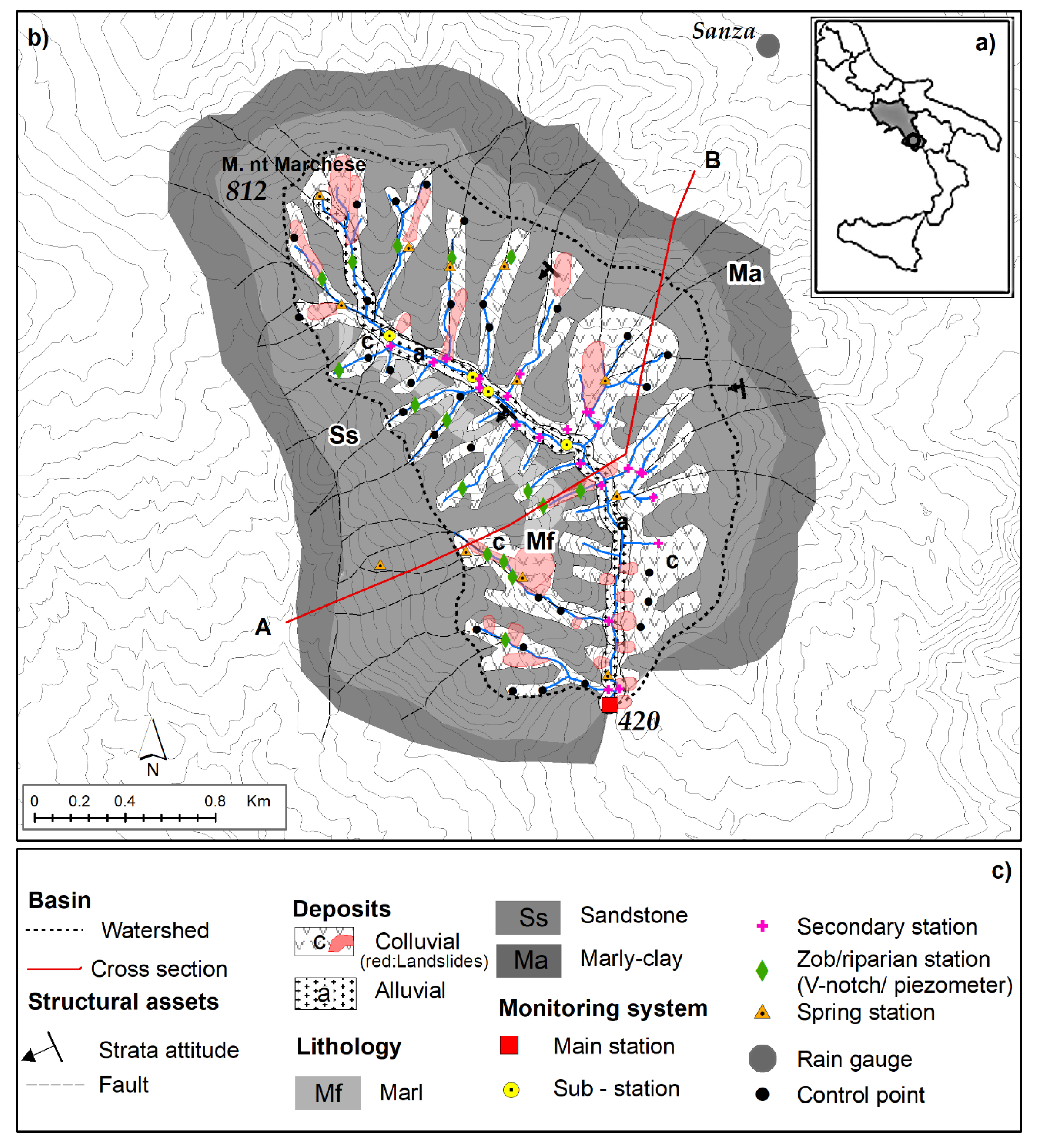
2.1. Study Area
2.2. Dataset
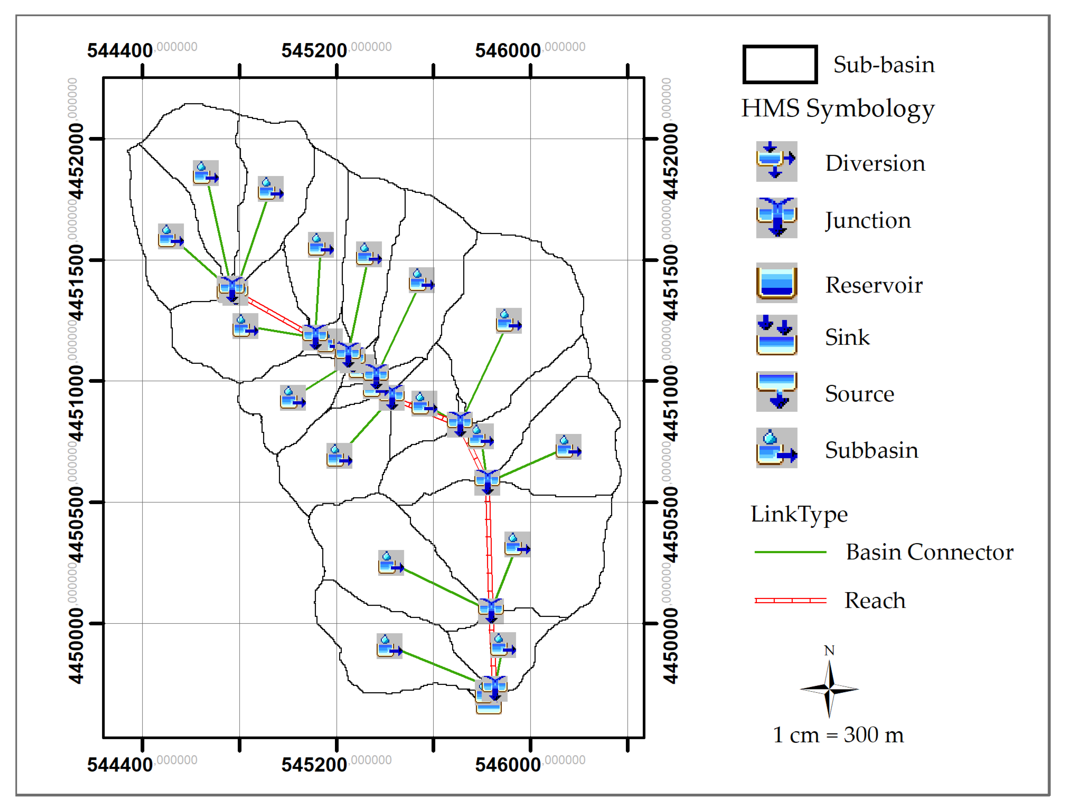
2.3. Hydrologic Modeling
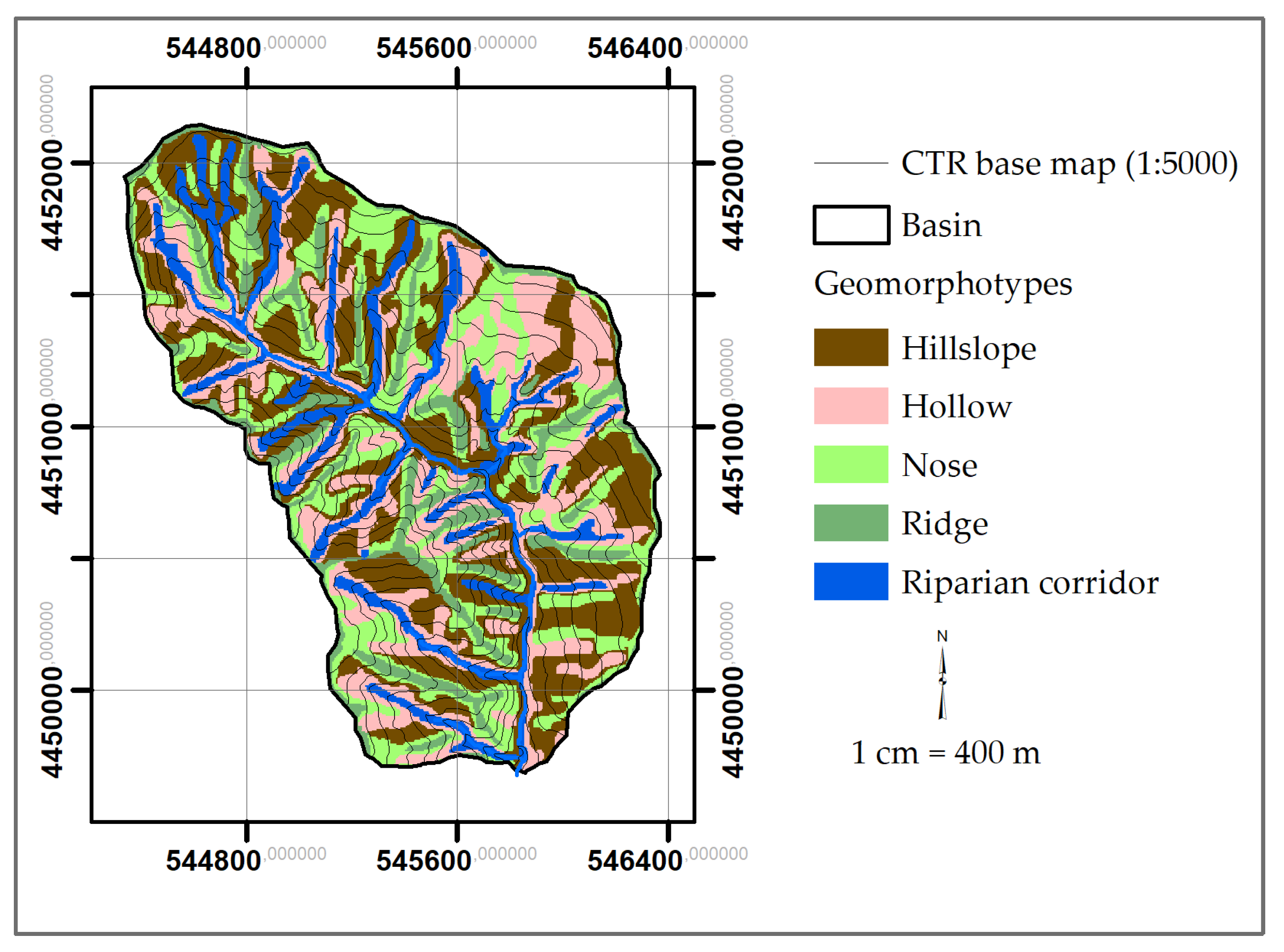
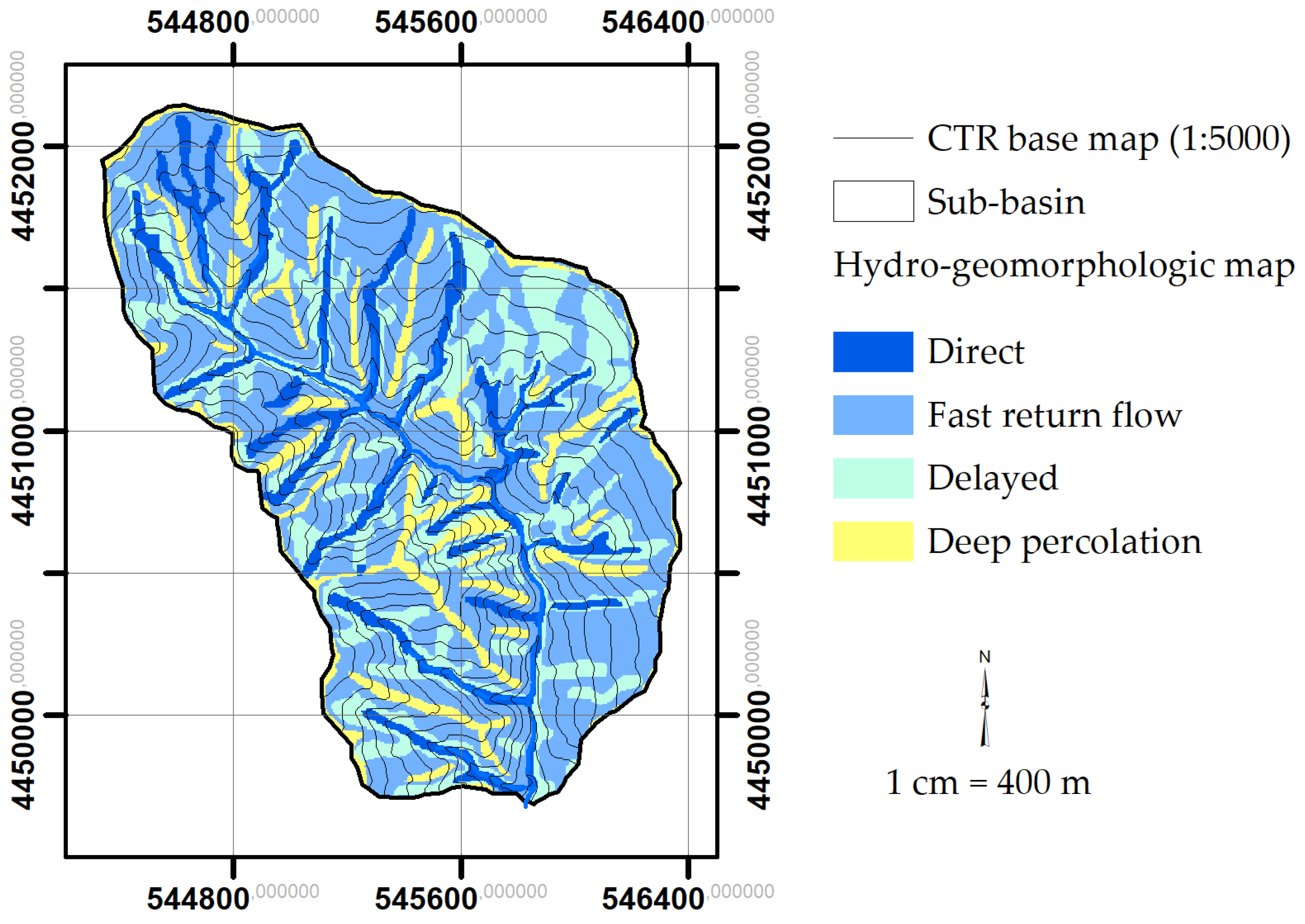
2.4. Hydro-Geomorphologic Modeling
2.5. Model Perfomance Evaluation
- Mean Absolute Error (MAE):
- 2.
- Mean Squared Error (MSE)
- 3.
- Root Mean Squared Error (RMSE)
- 4.
- Nash–Sutcliffe Efficiency coefficient (NSE)
- 5.
- Index of agreement (d)
3. Results and Discussions
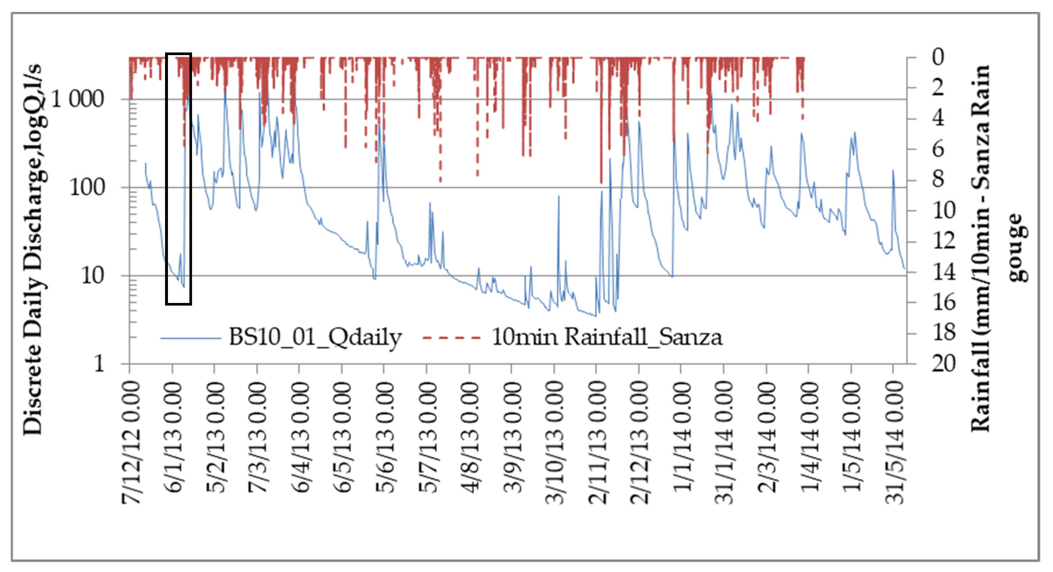
3.1. Recession Curve Analysis
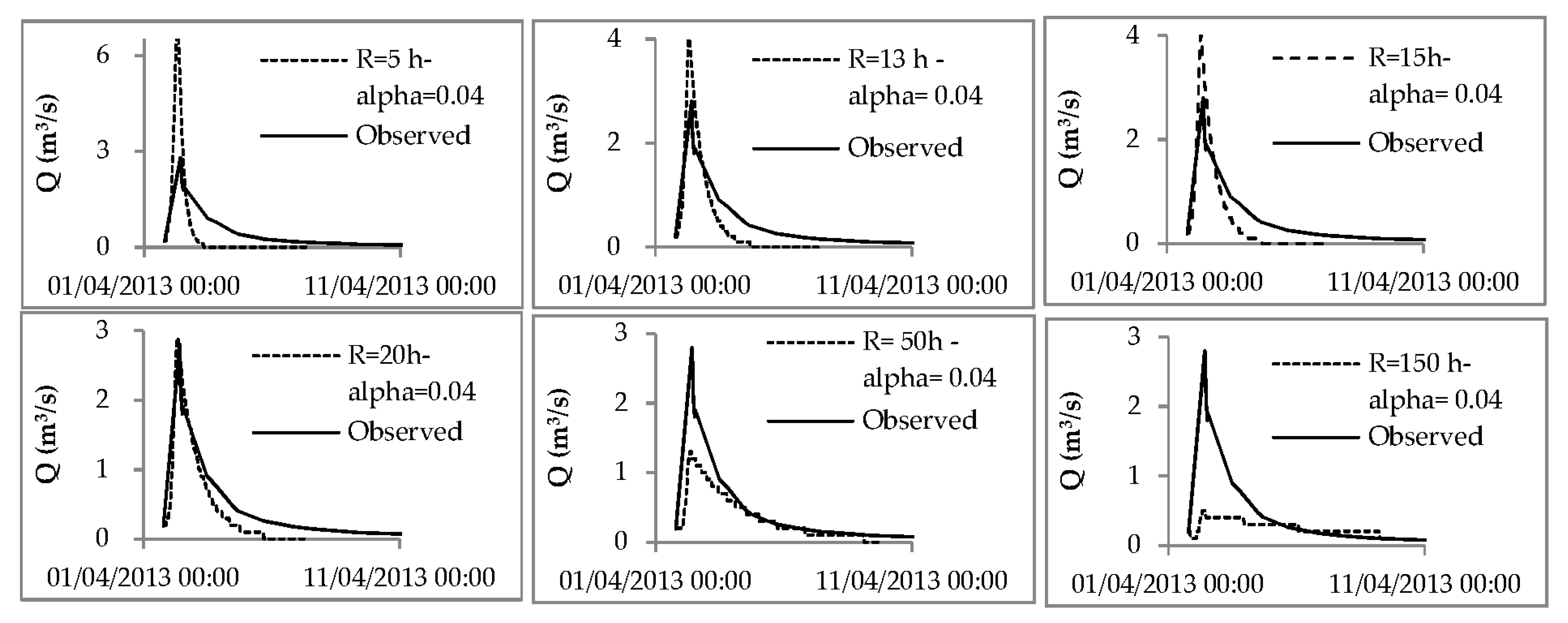
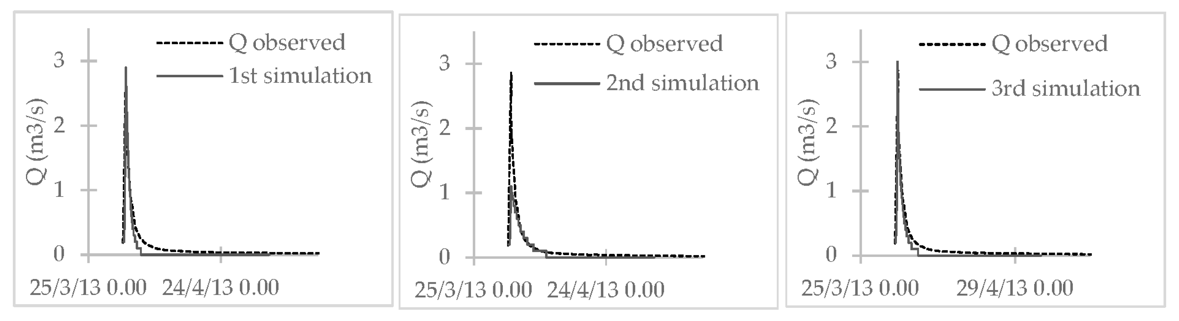
3.2. Lumped-Based Hydrologic Simulation
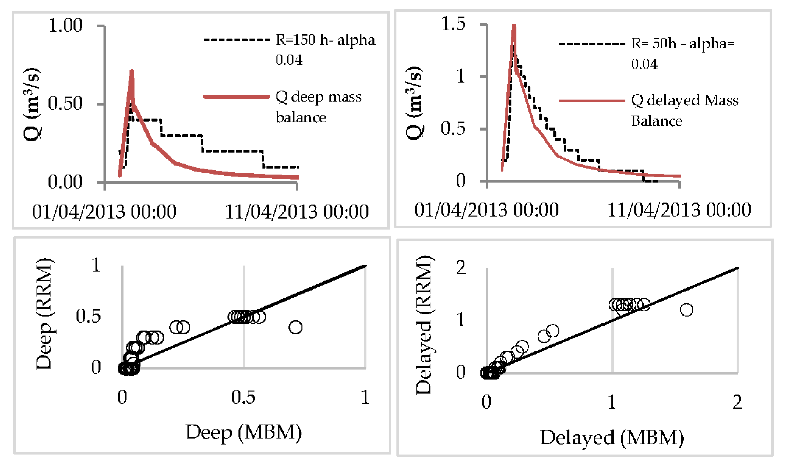
3.3. Distributed Rainfall–Runoff Simulations
3.3.1. Hydro-Geomorphologic Map
3.3.2. Hydro-Geomorphological Rainfall–Runoff Simulation
4. Conclusions
Author Contributions
Funding
Institutional Review Board Statement
Informed Consent Statement
Acknowledgments
Conflicts of Interest
References
- Borga, M.; Stoffel, M.; Marchi, L.; Marra, F.; Jakob, M. Hydrogeomorphic response to extreme rainfall in headwater systems: Flash floods and debris flows. J. Hydrol. 2014, 518, 194–205. [Google Scholar] [CrossRef]
- Portugués-Mollá, I.; Bonache-Felici, X.; Mateu-Bellés, J.F.; Marco-Segura, J.B. A GIS-Based Model for the analysis of an urban flash flood and its hydro-geomorphic response. The Valencia event of 1957. J. Hydrol. 2016, 541, 582–596. [Google Scholar] [CrossRef]
- Sidle, R.C.; Tsuboyama, Y.; Noguchi, S.; Hosoda, I.; Motohisa, F.; Shimuizu, T. Stormflow generation in steep forested headwater: A linked hydrogeomorphic paradigm. Hydrol. Process. 2000, 14, 369–385. [Google Scholar] [CrossRef]
- Sidle, R.C.; Kim, K.; Tsuboyama, Y.; Hosoda, I. Development and application of a simple hydrogeomorphic model for headwater catchments. Water Resour. Res. 2011, 47. [Google Scholar] [CrossRef]
- Kim, K.; Sidle, R.C.; Tsuboyama, Y. Modeling runoff dynamics from zero-order basins: Implications for hydrological pathways. Hydrol. Res. Lett. 2011, 5, 6–10. [Google Scholar] [CrossRef]
- Beven, K.J. Rainfall–Runoff Modelling: The Primer. Available online: http://public.eblib.com/choice/publicfullrecord.aspx?p=822562. (accessed on 25 October 2020).
- Bloschl, G. Rainfall–runoff Modeling of Ungauged Catchments. In Encyclopedia of Hydrological Sciences; Anderson, M.G., Ed.; John Wiley & Sons, Ltd.: Hoboken, NJ, USA, 2005; p. 19. [Google Scholar]
- James, L.D. Selection, calibration, and testing of hydrologic models. In Hydrologic Modeling of Small Watersheds; American Society of Agricultural Engineers: St. Joseph, MO, USA, 1982; pp. 437–472. [Google Scholar]
- Razaq, S.; Ismail, T.; Arien, H.; Awan, U.; Alamgir, M.; Hadipour, S. Streamflow prediction in ungauged catchments in the east coast of Peninsular Malaysia using multivariate statistical techniques. J. Teknol. 2016, 78. [Google Scholar] [CrossRef]
- Salinas, J.L.; Laaha, G.; Rogger, M.; Parajka, J.; Viglione, A.; Sivapalan, M.; Blöschl, G. Comparative assessment of predictions in ungauged basins & ndash; Part 2: Flood and low flow studies. Hydrol. Earth Syst. Sci. 2013, 17, 2637–2652. [Google Scholar] [CrossRef]
- Kite, G.W.; Kouwen, N. Watershed modeling using land classifications. Water Resour. Res. 1992, 28, 3193–3200. [Google Scholar] [CrossRef]
- Flügel, W.-A. Delineating hydrological response units by geographical information system analyses for regional hydrological modelling using PRMS/MMS in the drainage basin of the River Bröl, Germany. Hydrol. Process. 1995, 9, 423–436. [Google Scholar] [CrossRef]
- Liang, X.; Lettenmaier, D.P.; Wood, E.F.; Burges, S.J. A simple hydrologically based model of land surface water and energy fluxes for general circulation models. J. Geophys. Res. Atmos. 1994, 99, 14415–14428. [Google Scholar] [CrossRef]
- Jain, S.K.; Kumar, N.; Ahmad, T.; Kite, G.W. SLURP model and GIS for estimation of runoff in a part of Satluj catchment, India. Hydrol. Sci. J. 1998, 43, 875–884. [Google Scholar] [CrossRef]
- Becker, A.; Braun, P. Disaggregation, aggregation and spatial scaling in hydrological modelling. J. Hydrol. 1999, 217, 239–252. [Google Scholar] [CrossRef]
- Wooldridge, S.; Kalma, J. Regional-scale hydrological modelling using multiple-parameter landscape zones and a statistical water balance model. Hydrol. Earth Syst. Sci. 2001, 5. [Google Scholar] [CrossRef]
- Wood, E.F.; Sivapalan, M.; Beven, K.; Band, L. Effects of spatial variability and scale with implications to hydrologic modeling. J. Hydrol. 1988, 102, 29–47. [Google Scholar] [CrossRef]
- Reggiani, P.; Sivapalan, M.; Majid Hassanizadeh, S. A unifying framework for watershed thermodynamics: Balance equations for mass, momentum, energy and entropy, and the second law of thermodynamics. Adv. Water Resour. 1998, 22, 367–398. [Google Scholar] [CrossRef]
- Zhang, G.P.; Savenije, H.H.G.; Fenicia, F.; Pfister, L. Modelling subsurface storm flow with the Representative Elementary Watershed (REW) approach: Application to the Alzette River Basin. Hydrol. Earth Syst. Sci. 2006, 10, 937–955. [Google Scholar] [CrossRef]
- Demaria, E.M.; Nijssen, B.; Wagener, T. Monte Carlo sensitivity analysis of land surface parameters using the Variable Infiltration Capacity model. J. Geophys. Res. Atmos. 2007, 112. [Google Scholar] [CrossRef]
- Gou, J.; Miao, C.; Duan, Q.; Tang, Q.; Di, Z.; Liao, W.; Wu, J.; Zhou, R. Sensitivity Analysis-Based Automatic Parameter Calibration of the VIC Model for Streamflow Simulations Over China. Water Resour. Res. 2020, 56, e2019WR025968. [Google Scholar] [CrossRef]
- Chawla, I.; Mujumdar, P.P. Partitioning uncertainty in streamflow projections under nonstationary model conditions. Adv. Water Resour. 2018, 112, 266–282. [Google Scholar] [CrossRef]
- Greuell, W.; Franssen, W.H.P.; Biemans, H.; Hutjes, R.W.A. Seasonal streamflow forecasts for Europe—Part I: Hindcast verification with pseudo- and real observations. Hydrol. Earth Syst. Sci. 2018, 22, 3453–3472. [Google Scholar] [CrossRef]
- Niraula, R.; Meixner, T.; Dominguez, F.; Bhattarai, N.; Rodell, M.; Ajami, H.; Gochis, D.; Castro, C. How Might Recharge Change Under Projected Climate Change in the Western U.S.? Geophys. Res. Lett. 2017, 44, 10, 407–410, 418. [Google Scholar] [CrossRef] [PubMed]
- Zhang, Q.; Manzoni, S.; Katul, G.; Porporato, A.; Yang, D. The hysteretic evapotranspiration—Vapor pressure deficit relation. J. Geophys. Res. Biogeosciences 2014, 119, 125–140. [Google Scholar] [CrossRef]
- Cuomo, A. Il Contributo Della Idro-Geomorfologia Nella Valutazione Delle Piene in Campania; University of Salerno: Fisciano, Italy, 2012. [Google Scholar]
- Dramis, F.; Guida, D.; Cestari, A. Chapter Three-Nature and Aims of Geomorphological Mapping. In Developments in Earth Surface Processes; Smith, M.J., Paron, P., Griffiths, J.S., Eds.; Elsevier: Amsterdam, The Netherlands, 2011; Volume 15, pp. 39–73. [Google Scholar]
- Guida, D.; Palmieri, V.; Paron, P.; Siervo, V. The Salerno University Geomorphological Informative Mapping System (GmIS_UniSa): Application to a polygenetic Mediterranean landscape (Cilento and Vallo di Diano European Geopark). In Proceedings of the IAG/AIG International Workshop on Objective Geomorphological Representation Models: Breaking through a New Geomorphological Mapping Frontier, Salerno, Italy, 15–19 October 2012; pp. 73–77. [Google Scholar]
- Cuomo, A.; Guida, D. Using hydro-chemograph analyses to reveal runoff generation processes in a Mediterranean catchment. Hydrol. Process. 2016, 30, 4462–4476. [Google Scholar] [CrossRef]
- Guida, D.; Cuomo, A.; Palmieri, V. Using object-based geomorphometry for hydro-geomorphological analysis in a Mediterranean research catchment. Hydrol. Earth Syst. Sci. 2016, 20, 3493–3509. [Google Scholar] [CrossRef]
- Cuomo, A.; Guida, D. Discharge-Electrical Conductivity Relationship in the Ciciriello Torrent, a Reference Catchment of the Cilento, Vallo Diano and Alburni European Geopark (Southern Italy); Rendiconti Online Societa Geologica Italiana: Roma, Italy, 2013; Volume 28, pp. 36–40. [Google Scholar]
- Guida, D.; Cuomo, A. Using discharge-electrical conductivity relationship in a Mediterranean catchment: The T. Ciciriello in the Cilento, Vallo Diano and Alburni European Geopark (Southern Italy). In Proceedings of the Engineering Geology for Society and Territory, Torino, Italy, 15–19 September 2014; pp. 201–205. [Google Scholar]
- Blasi, C.; Capotorti, G.; Copiz, R.; Guida, D.; Mollo, B.; Smiraglia, D.; Zavattero, L. Classification and mapping of the ecoregions of Italy. Plant Biosyst. Int. J. Deal. All Asp. Plant Biol. 2014, 148, 1255–1345. [Google Scholar] [CrossRef]
- Bonardi, G.; Amore, F.O.; Ciampo, G.; De Capoa, P.; Miconnet, P.; Perrone, V. Il complesso liguride Auct.: Stato delle conoscenze e problemi sualla sua evoluzione Pre-Appenninica ed i suoi rapporti con l’arco calabro. Mem. Soc. Geol. Ital. 1988, 41, 17–35. [Google Scholar]
- Guida, D.; Cuomo, A.; Longobardi, A.; Villani, P. Geohydrology of a Reference Mediterranean Catchment (Cilento UNESCO Geopark, Southern Italy). Appl. Sci. 2020, 10, 4117. [Google Scholar] [CrossRef]
- Cascini, L.; Cuomo, S.; Guida, D. Typical source areas of May 1998 flow-like mass movements in the Campania region, Southern Italy. Eng. Geol. 2008, 96, 107–125. [Google Scholar] [CrossRef]
- Hewlett, J.D.; Hibbert, A.R. Factors affecting the response of small forested watersheds to precipitation in humid regions. Forest Hydrol. 1967, 1, 275–290. [Google Scholar]
- USACE. HEC-HMS Hydrologic Modeling System User’s Manual; USACE: Davis, CA, USA, 2000.
- Fleming, M.; Neary, V. Continuous hydrologic modeling study with the hydrologic modeling system. J. Hydrol. Eng. 2004, 9, 175–183. [Google Scholar] [CrossRef]
- Moghadas, S. Long-term Water Balance of an Inland River Basin in an Arid Area, North-Western China; Lund Institute of Technology, Lund University: Lund, Sweden, 2009. [Google Scholar]
- Wang, J.; Hong, Y.; Gourley, J.; Adhikari, P.; Li, L.; Su, F. Quantitative assessment of climate change and human impacts on long-term hydrologic response: A case study in a sub-basin of the Yellow River, China. Int. J. Climatol. 2010, 30, 2130–2137. [Google Scholar] [CrossRef]
- USACE. HEC-HMS Hydrologic Modeling System User’s Manual; USACE: Davis, CA, USA, 2008.
- Maillet, E. Essais D’hydraulique Souterraine & Fluviale; Librairie Sci., A. Hermann: Paris, France, 1905; 218p. [Google Scholar]
- Jakada, H.; Chen, Z.; Luo, M.; Zhou, H.; Wang, Z.; Habib, M. Watershed Characterization and Hydrograph Recession Analysis: A Comparative Look at a Karst vs. Non-Karst Watershed and Implications for Groundwater Resources in Gaolan River Basin, Southern China. Water 2019, 11, 743. [Google Scholar] [CrossRef]
- Scharffenberg, W.; Ely, P.; Daly, S.; Fleming, M.; Pak, J. Hydrologic modeling system (hec-hms): Physically-based simulation components. In Proceedings of the 2nd Joint Federal Interagency Conference, Las Vegas, NV, USA, 27 June–1 July 2010. [Google Scholar]
- Longobardi, A.; Villani, P.; Guida, D.; Cuomo, A. Hydro-geo-chemical streamflow analysis as a support for digital hydrograph filtering in a small, rainfall dominated, sandstone watershed. J. Hydrol. 2016, 539, 177–187. [Google Scholar] [CrossRef]
- Keller, E.A.; Pinter, N. Active Tectonics: Earthquake, Uplift, and Landscape; Prentice Hall: Upper Saddle River, NJ, USA, 1996; p. 338. [Google Scholar]
- Latron, J.; Soler, M.; Llorens, P.; Gallart, F. Spatial and temporal variability of the hydrological response in a small Mediterranean research catchment (Vallcebre, Eastern Pyrenees). Hydrol. Process. 2008, 22, 775–787. [Google Scholar] [CrossRef]


| Storm Event | IPmax( mm/h) | Pt (mm) | Qo (l/s) | Qmax (l/s) | API15 (mm) | RC * |
|---|---|---|---|---|---|---|
| 1/4/13 10.00 | 4.8 | 65.8 | 189 | 2200 | 53 | 0.9 |
| Landform, Component, or Element | Geomorphotype [27] | Hydro-Geomorphological Behaviour | Hydro-Geomorphotype (HGmT in [26]) | EC Range (μS/cm) [35]) |
|---|---|---|---|---|
| Upland, summit, peak, crest | Ridge | Groundwater recharge on bare bedrock and dominant excess infiltration runoff after storm | Deep percolation | 250–300 <100 |
| Shoulder, side slope | Nose | Shallow soil, groundwater recharge area, prevalent excess infiltration runoff | Deep percolation | 250–300 <100 |
| Scarps, back-slope, foot-slope, wash-slope, talus | Hillslope | Debris, deep soil, shallow aquifer, excess saturation excess and sub-surficial runoff | Fast return flow | 120–180 |
| Glen, swallet, scar | Hollow | Deep soil, shallow aquifer, prevalently excess saturation, delayed runoff production | Delayed return flow | 200–220 |
| V-shaped stream, gully, bank, stream bed | Riparian corridor | Shallow soil, groundwater discharge, prevalently sub-surface, delayed return flow and groundwater ridging | Direct | 80–120 |
| α (1/Day) | Mean | Max | Min | SD |
|---|---|---|---|---|
| Direct runoff (α1) | 5.40 | 6.90 | 2.50 | 2.05 |
| Quick return flow 1 (α2) | 0.52 | 0.80 | 0.36 | 0.14 |
| Delayed return flow (α3) | 0.161 | 0.21 | 0.11 | 0.038 |
| Deep percolation (α4) | 0.04 | 0.09 | 0.02 | 0.02 |
| Runoff Mechanisms | t (h) |
|---|---|
| Direct runoff | 5.26 |
| Quick return flow | 49.61 |
| Delayed return flow | 157.51 |
| Deep percolation | 729.76 |
| Ab (km2) | La (km) | Zm (m) | Z0 (m) | tc (h) |
|---|---|---|---|---|
| 3.04 | 2.53 | 617.15 | 393.6 | 0.9 |
| Sub-Basin | Channel | Ab (km2) | La (km) | Zm (m) | Z0 (m) | tc (h) |
|---|---|---|---|---|---|---|
| W240 | R20 | 0.167 | 0.449 | 715.89 | 583.5 | 0.25 |
| W250 | R40 | 0.155 | 0.356 | 705.48 | 579.2 | 0.23 |
| W260 | R10 | 0.153 | 0.205 | 682.23 | 582.9 | 0.23 |
| W270 | R30 | 0.002 | 0.019 | 597.32 | 579.4 | 0.06 |
| W280 | R60 | 0.134 | 0.210 | 664.31 | 541.4 | 0.20 |
| W290 | R50 | 0.186 | 0.415 | 619.54 | 541.2 | 0.33 |
| W300 | R80 | 0.132 | 0.250 | 667.16 | 528.3 | 0.19 |
| W310 | R120 | 0.190 | 0.378 | 647.95 | 520.1 | 0.26 |
| W320 | R70 | 0.021 | 0.166 | 562.50 | 527.8 | 0.18 |
| W330 | R150 | 0.306 | 0.415 | 641.24 | 499.0 | 0.30 |
| W340 | R90 | 0.001 | 0.028 | 532.60 | 526.8 | 0.07 |
| W350 | R100 | 0.110 | 0.088 | 637.45 | 526.8 | 0.17 |
| W360 | R110 | 0.018 | 0.130 | 549.44 | 519.3 | 0,17 |
| W370 | R130 | 0.028 | 0.122 | 565.89 | 514.0 | 0.15 |
| W380 | R160 | 0.156 | 0.222 | 635.06 | 514.2 | 0.22 |
| W390 | R140 | 0.087 | 0.341 | 558.01 | 497.9 | 0.27 |
| W400 | R170 | 0.178 | 0.312 | 587.31 | 474.0 | 0.25 |
| W410 | R180 | 0.171 | 0.150 | 607.88 | 474.3 | 0.20 |
| W420 | R200 | 0.341 | 0.586 | 536.61 | 426.8 | 0.38 |
| W430 | R190 | 0.228 | 0.514 | 602.15 | 427.7 | 0.25 |
| W440 | R220 | 0.093 | 0.361 | 460.84 | 396.3 | 0.27 |
| W450 | R210 | 0.179 | 0.410 | 572.33 | 396.7 | 0.22 |
| W460 | R230 | 0.006 | 0.066 | 408.43 | 393.6 | 0.13 |
| Sub-Basin | HGmIdeep | HGmI delayed | HGmIast | HGmIdirect |
|---|---|---|---|---|
| W240 | 0.11 | 0.04 | 0.60 | 0.25 |
| W250 | 0.15 | 0.20 | 0.48 | 0.17 |
| W260 | 0.11 | 0.32 | 0.46 | 0.12 |
| W270 | 0.37 | 0.35 | 0.28 | |
| W280 | 0.11 | 0.24 | 0.55 | 0.10 |
| W290 | 0.09 | 0.20 | 0.60 | 0.11 |
| W300 | 0.10 | 0.41 | 0.30 | 0.19 |
| W310 | 0.11 | 0.44 | 0.29 | 0.15 |
| W320 | 0.17 | 0.22 | 0.52 | 0.10 |
| W330 | 0.06 | 0.41 | 0.43 | 0.11 |
| W340 | 0.42 | 0.58 | ||
| W350 | 0.19 | 0.16 | 0.37 | 0.28 |
| W360 | 0.05 | 0.02 | 0.78 | 0.15 |
| W370 | 0.15 | 0.29 | 0.51 | 0.05 |
| W380 | 0.10 | 0.25 | 0.51 | 0.14 |
| W390 | 0.19 | 0.21 | 0.52 | 0.08 |
| W400 | 0.25 | 0.31 | 0.29 | 0.16 |
| W410 | 0.09 | 0.21 | 0.62 | 0.07 |
| W420 | 0.12 | 0.17 | 0.63 | 0.08 |
| W430 | 0.10 | 0.25 | 0.53 | 0.13 |
| W440 | 0.06 | 0.18 | 0.69 | 0.06 |
| W450 | 0.16 | 0.28 | 0.43 | 0.13 |
| W460 | 0.01 | 0.37 | 0.41 | 0.21 |
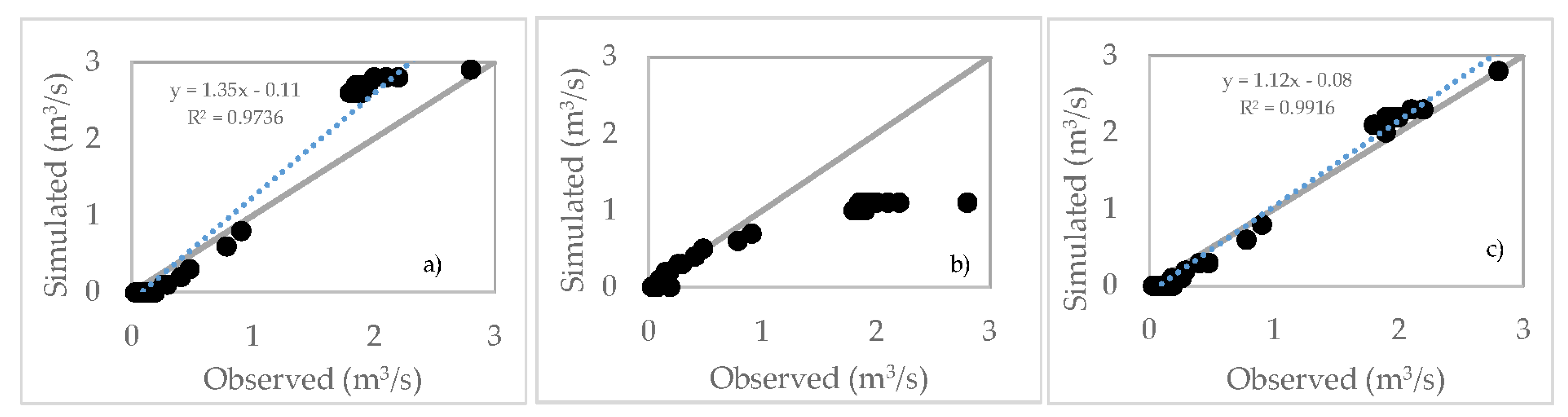
| Simulation | MAE | MSE | RMSE | NSE | d |
|---|---|---|---|---|---|
| 1 | 0.22 | 0.35 | 0.59 | 0.64 | 0.86 |
| 2 | 0.25 | 2.76 | 1.66 | 0.32 | 0.78 |
| 3 | 0.10 | 0.01 | 0.10 | 0.95 | 0.93 |
Publisher’s Note: MDPI stays neutral with regard to jurisdictional claims in published maps and institutional affiliations. |
© 2021 by the authors. Licensee MDPI, Basel, Switzerland. This article is an open access article distributed under the terms and conditions of the Creative Commons Attribution (CC BY) license (http://creativecommons.org/licenses/by/4.0/).
Share and Cite
Cuomo, A.; Guida, D. Hydro-Geomorphologic-Based Water Budget at Event Time-Scale in A Mediterranean Headwater Catchment (Southern Italy). Hydrology 2021, 8, 20. https://doi.org/10.3390/hydrology8010020
Cuomo A, Guida D. Hydro-Geomorphologic-Based Water Budget at Event Time-Scale in A Mediterranean Headwater Catchment (Southern Italy). Hydrology. 2021; 8(1):20. https://doi.org/10.3390/hydrology8010020
Chicago/Turabian StyleCuomo, Albina, and Domenico Guida. 2021. "Hydro-Geomorphologic-Based Water Budget at Event Time-Scale in A Mediterranean Headwater Catchment (Southern Italy)" Hydrology 8, no. 1: 20. https://doi.org/10.3390/hydrology8010020
APA StyleCuomo, A., & Guida, D. (2021). Hydro-Geomorphologic-Based Water Budget at Event Time-Scale in A Mediterranean Headwater Catchment (Southern Italy). Hydrology, 8(1), 20. https://doi.org/10.3390/hydrology8010020