Calibration of NSRP Models from Extreme Value Distributions

Abstract

In this work, the authors investigated the feasibility of calibrating a model which is suitable for the generation of continuous high-resolution rainfall series, by using only data from annual maximum rainfall (AMR) series, which are usually longer than continuous high-resolution data, or they are the unique available data set for many locations. In detail, the basic version of the Neyman–Scott Rectangular Pulses (NSRP) model was considered, and numerical experiments were carried out, in order to analyze which parameters can mostly influence the extreme value frequency distributions, and whether heavy rainfall reproduction can be improved with respect to the usual calibration with continuous data. The obtained results were highly promising, as the authors found acceptable relationships among extreme value distributions and statistical properties of intensity and duration for the pulses. Moreover, the proposed procedure is flexible, and it is clearly applicable for a generic rainfall generator, in which probability distributions and shape of the pulses, and extreme value distributions can assume any mathematical expression.

1. Introduction

Long continuous high-resolution series of rainfall are more and more necessary for many hydrological purposes, in particular for applications related to small urban catchments.

However, for many locations of interest, the sample sizes of continuous data with a high resolution are usually short, or they are not available, and only annual maximum rainfall (AMR) series exist, but they are often not so long at the finest time scales (1 or 5 min).

These usual data deficiencies, together with the necessity to obtain perturbed time series, that can be representative of future rainfall fields at hydrological scales, induced the development of stochastic rainfall generators (SRGs), which are characterized by simple mathematical formulations and low computational costs, thus allowing for the quick generation of large ensembles of long precipitation time series.

A review of all these SRGs is provided in [1,2]. In particular, many works [3,4,5,6,7,8,9] highlighted the capacity of a specific class of SRGs, i.e., the Poisson cluster models, to satisfactorily reproduce observed summary statistics, such as mean, variance, skewness, proportion of dry/wet periods, and k-lag autocorrelation values, of the continuous rainfall process at several fine time scales. Poisson cluster models mainly comprise Neyman–Scott and Bartlett–Lewis families, which perform equally well [10]. Many applications of these models regarded England [5,8,11,12,13], Scotland [14], Belgium [7], Switzerland [15], Germany [9], Spain [16], Ireland [16], South Africa [17], New Zealand [18], Australia [19,20,21], Greece [22], Italy [23,24], United States [3,4,23,25,26,27], and Korean Peninsula [28].

On the contrary, other works stated the inability of these models to reconstruct extreme values, as they usually underestimate these rainfall heights at hourly and sub-hourly scales (see e.g., [29]). Consequently, many variants were proposed, related to (i) a change of model structure [9,30,31,32], (ii) inclusion of disaggregation techniques [33,34,35,36], (iii) model fitting with more information about the variability of precipitation [37]. However, many of these proposals implied an increasing parameterization, which limited their adoption, in particular for locations with very short samples.

In order to overcome these problems, censored versions [38] were introduced. They only model rainfall values over a prefixed threshold (i.e., there is only one more parameter to be estimated) and allow for a better reproduction of heavy portions of the hyetographs, because skewness (which usually assumes very high values at fine scales) and the proportion of dry/wet periods are both considered as unimportant. However, due to these latter aspects, these censored approaches are unsuitable for generating continuous time series as well, because a rainfall value below the censor is automatically set to zero, and then it is impossible to obtain a good reproduction of the proportion of dry/wet periods, which can be of interest for some applications.

From the above briefly discussed state-of-art for SRGs, two main key aspects emerge:

• The sample size of continuous rainfall series with a high resolution plays a crucial role for a robust calibration of SRGs. In many locations, this sample size is very short and/or only AMR series are available.
• The basic versions of SRGs usually underestimate extreme values at fine scales. Many attempts at improving the modeling were carried out, but they implied an unsuitable over parameterization for short sample sizes or an inability to reconstruct other features, such as dry/wet ratios.

In this context, the goal of this work is to answer to the following questions, which could arise from the above considerations:

(a)

Is it possible to calibrate a SRG by only using AMR series, which are usually more and more longer than continuous data with a high-resolution for many locations? Even, AMR series are the unique available data set for some locations.

(b)

If so, for a specific SRG are there some parameters which mostly influence the extreme value distributions?

In detail, the authors focused on the basic version of the single-site Neyman–Scott Rectangular Pulses model (NSRP [3,11,39]) and they carried out numerical experiments in order to reply to the previous questions.

The paper is organized as follows:

• In Section 2, the authors provided a brief overview of the NSRP model and described the adopted calibration and validation procedures, in order to derive possible relationships among extreme value distributions and NSRP parameters.
• The obtained results, from calibration and validations procedures, are illustrated in Section 3.
• Section 4 regards discussion about results and future developments.

2. Materials and Methods

2.1. Brief Theoretical Description of NSRP Model

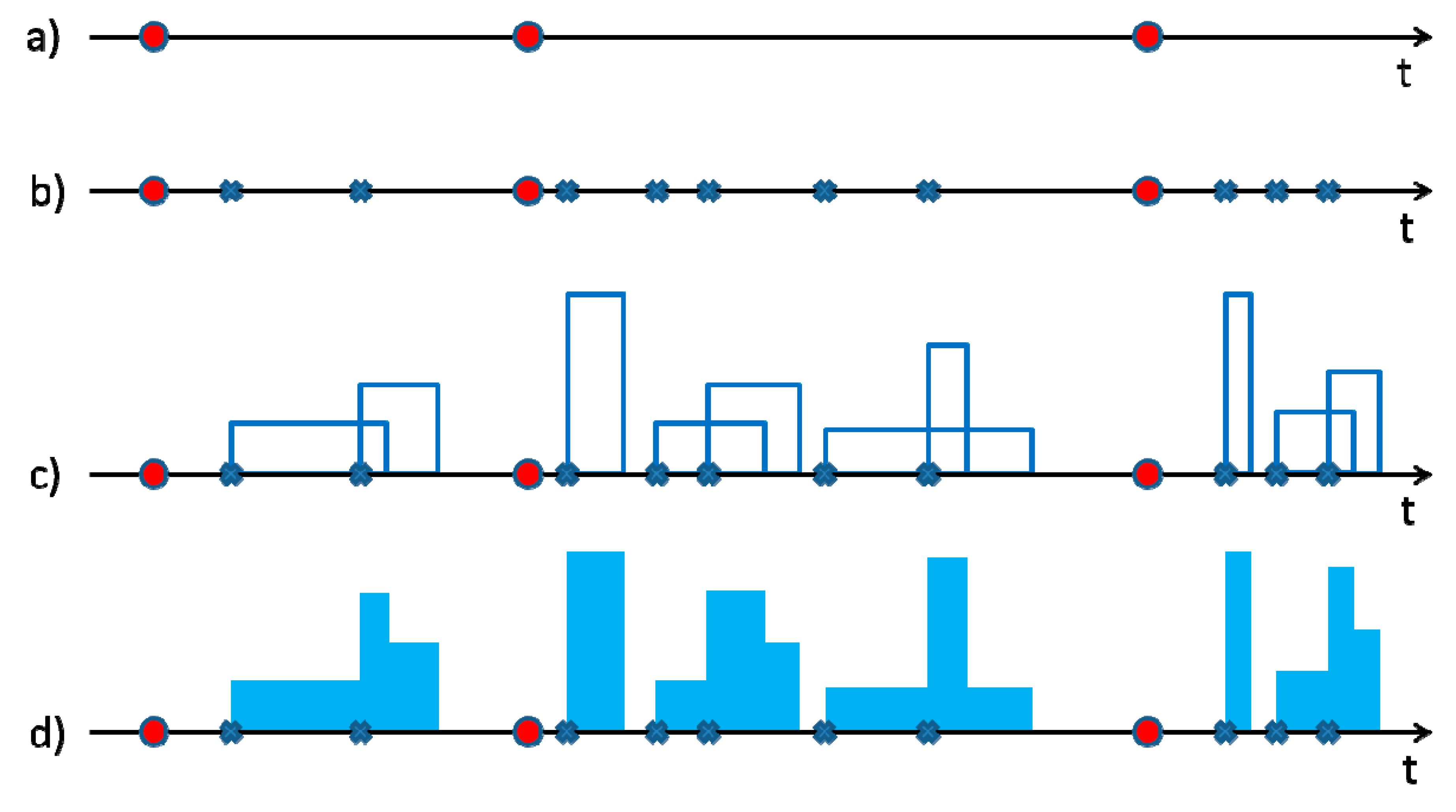
In this work, the authors focused their attention on the single-site Neyman–Scott Rectangular Pulses (NSRP [3,11,39]) model, which is based on a clustering approach: rainfall is associated with clusters of rain cells making up storm events. In detail, the basic formulation is described below (see also Figure 1):

• It is assumed that the number of storms is a homogeneous Poisson random variable. This means that the inter-arrivals, $T_s$, between the origins of two consecutive storms are independent and identically distributed, and they follow an exponential distribution:

  $$P_{T_S}\left(t_S\right)=P\left[T_s\le t_s\right]=1-e^{-\lambda \cdot t_S},$$

  (1)

  where $P\left[T_s\le t_s\right]$ is the probability for the event $T_s\le t_s$ and $1/\lambda$ represents the mean value for the inter-arrivals.
• A number, $M$, of rain cells (also named bursts or pulses) is associated with each storm origin; $M$ is usually considered as geometric or Poisson distributed. In this work, a geometric distribution is assumed and, with the aim of having at least one burst for each storm, the random variable $C=M-1$ is used, with $E\left[C\right]=\theta -1$, so that $E\left[M\right]=\theta$ and:

  $$P_C\left(c\right)=\frac{1}{\theta }\cdot {\left(1-\frac{1}{\theta }\right)}^c.$$

  (2)
• With respect to the associated storm origin, each burst origin occurs after a waiting time, W, which is assumed as an exponentially distributed variable with parameter ${\beta }_W$ and $E\left[W\right]=1/{\beta }_W$:

  $$P_W\left(w\right)=P\left[W\le w\right]=1-e^{-{\beta }_W\cdot w}.$$

  (3)
• Each burst has a rectangular shape, with an intensity I and a duration D which are both considered as exponential distributed, with parameters ${\beta }_I$ and ${\beta }_D$, respectively, and $E\left[I\right]=1/{\beta }_I$, $E\left[D\right]=1/{\beta }_D$:

  $$P_I\left(i\right)=P\left[I\le i\right]=1-e^{-{\beta }_I\cdot i},$$

  (4)

  $$P_D\left(d\right)=P\left[D\le d\right]=1-e^{-{\beta }_D\cdot d}.$$

  (5)
• The total precipitation intensity, $Y\left(t\right),$ at time t is then calculated as the sum of the intensities which are related to the active bursts at time t:

  $$Y\left(t\right)={\displaystyle \underset{0}{\overset{+\infty }{\int }}{I}_{t-u}\left(u\right)dM\left(t-u\right)},$$

  (6)

  where $I_{t-u}\left(u\right)$ is the intensity of a single rectangular pulse at time u and $M\left(t\right)$ is the counting process of the burst occurrences. Then, the aggregated process, i.e., the rainfall height $H_j^{\left(\tau \right)}$ cumulated on the temporal $\tau$ resolution and related to the time interval j is:

  $$H_j^{\left(\tau \right)}={\displaystyle \underset{\left(j-1\right)\cdot \tau }{\overset{j\cdot \tau }{\int }}Y\left(t\right)}\cdot dt.$$

  (7)

Therefore, the basic version of a NSRP model has five parameters. Calibration is usually carried out by minimizing an objective function, which is defined as the sum of residuals (normalized or not) between the considered (by users) statistical properties of the observed data at chosen resolutions and their theoretical expressions. The statistical properties are typically referred to high-resolution continuous time series (e.g., 5 min rainfall time series): mean, variance, k-lag autocorrelation for ${\mathrm{H}}_j^{\left(\tau \right)}$ at several values of $\tau$ [40] can be mentioned as examples. However, the sample size of these datasets is usually short (at most 15–20 years of records), and it is not very suitable for obtaining robust estimations, even more so when a specific five-parameter set is considered for each month or season, in order to take into account the seasonality of the process. Moreover, as already mentioned in Section 1, currently many high-resolution time series from rain gauges usually regard only annual maximum rainfall (AMR) data; from these, it is impossible to obtain information about the above-listed statistical properties of the continuous process, and then it could seem unthinkable to obtain a NSRP calibration from AMR data.

In this context, the authors investigated the possibility/feasibility of calibrating the basic version of a NSRP model (to be preferred for reasons concerning parametric parsimony) from AMR series, also in order to improve the performance regarding reconstruction of extreme events, which are generally underestimated when continuous data are used (see e.g., [29]).

With this goal, Section 2.1 and Section 2.2 regard the description of the adopted calibration and validation procedures, respectively.

2.2. Calibration Procedure

Numerical experiments, which are below described, were carried out. Specifically, the authors used long synthetic continuous time series; this choice allows for obtaining more reliable estimations for possible relationships among (in this specific case) statistical properties of continuous process and those of the associated extreme values. Obviously, this analysis could be affected by high uncertainties if observed data were used, because of their limited sample sizes (mainly of the continuous time series).

First of all, as a simple hypothesis, the rainfall process was assumed as stationary, postponing to future works the modeling of seasonality (thus considering the process as cyclostationary) and trend analyses (for climate change contexts). This simple hypothesis allows for avoiding, in a framework of parametric parsimony, the use of a specific five-parameter set for each month or season. Moreover, although it could seem too strong and unrealistic, it is coherent with the extreme value theory [41], from which the probability distributions (EV1, EV2, EV3, GEV, etc.) are derived by considering, inside a fixed temporal block (usually a year), a sequence of values (whence the maximum is extracted) as independent and identically distributed random variables, i.e., without any seasonality feature.

In detail, the adopted calibration procedure can be explained in the following steps:

• Each NSRP parameter was considered as a uniform random variable, with a specific variation range, according to [40,42] (see

  Table 1. Assumed parameter ranges of variation for the adopted basic version of NSRP model.

  NSRP Parameter	Min. Value	Max. Value
  $1/\lambda$ (h)	120	360
  $\theta$ (-)	2	10
  ${1/\beta }_W$ (h)	5	24
  ${1/\beta }_I$ (mm/h)	5	15
  ${1/\beta }_D$ (h)	0.1	0.6

  ), and all the parameters were assumed as independent among them, for simplicity.
• Then, 1000 five-parameter sets were generated with a Monte Carlo approach [43], and, for each set, a 500-year continuous time series of 1 min rainfall heights was simulated, from which AMR series, related to 5, 15, 30, and 60 min, were extracted. The choice of generating only one long realization is according to the ergodicity property for a stationary stochastic process [43,44].
• Although analytical expressions of probability distributions do not exist for AMR series from the basic version of a NSRP model, they can be approximated with an EV1 distribution [45]:

  $$P_H\left(h\right)=P\left[H\le h\right]=e^{-e^{-\alpha \cdot \left(h-\epsilon \right)}}$$

  (8)

  with $\alpha >0,\epsilon >0$ and H is the annual maximum rainfall height at a specific time-resolution.
  The parameters $\alpha$ and $\epsilon$ are related to the theoretical mean, $\mu$, and standard deviation, $\sigma$, of H in the following way [43]:

  $$\mu =\epsilon +\frac{n_e}{\alpha },$$

  (9)

  $$\sigma =\frac{\pi }{\sqrt{6}\cdot \alpha },$$

  (10)

  where $n_e$ denotes the Euler constant, approximately equal to 0.5772. For each considered duration (5, 15, 30, and 60 min), the EV1 parameter set $\underset{\_}{T}=\left(\alpha ,\epsilon \right)$ was estimated by using the maximum-likelihood (ML) method [43].
• The final step regarded the investigation of possible relationships among each NSRP parameter from the set $\underset{\_}{\Theta }=\left(\lambda ,\theta ,{\beta }_W,{\beta }_I,{\beta }_D\right)$ with the sets $\underset{\_}{T}$, estimated into Step 3 for the considered durations (5, 15, 30, and 60 min).

Concerning Step 4, several performance measures can be adopted (e.g., see [46]). In this case, the authors used the minimization of the mean square error ($MSE$):

$$MSE=\frac{1}{N}{\displaystyle \sum _{i=1}^N{\left(y_i-y_i^{*}\right)}^2},$$

(11)

where $N$ is the number of pairs regarding observed and modeled data, $y_i$ is the i-th observed value and $y_i^{*}$ is the i-th modeled value. In this work $N$= 1000, while $y_i$ and $y_i^{*}$ correspond to, respectively, the sample estimates and the reconstructed values (by using relationships with the sets $\underset{\_}{T}$) for each NSRP parameter. $MSE$ is usually associated with the coefficient of determination, $R^2$:

$$R^2={\left[\frac{{\displaystyle \sum _{i=1}^N\left(y_i-\overline{y}\right)\left(y_i^{*}-{\overline{y}}^{*}\right)}}{\sqrt{{\displaystyle \sum _{i=1}^N{\left(y_i-\overline{y}\right)}^2}}\sqrt{{{\displaystyle \sum _{i=1}^N\left(y_i^{*}-{\overline{y}}^{*}\right)}}^2}}\right]}^2$$

(12)

where $\overline{y}$ and ${\overline{y}}^{*}$ are the mean values for $y_i$ and $y_i^{*}$, respectively. The ranges of variation are (0, +∞) for MSE and (0, 1) for $R^2$. Moreover, low values of $MSE$ are associated with high values of $R^2$ and vice versa.

In an equivalent way, a user can carry out the maximization of the Nash–Sutcliffe Efficiency coefficient ($NSE$):

$$NSE=1-\frac{\frac{1}{N}{\displaystyle \sum _{i=1}^N{\left(y_i-y_i^{*}\right)}^2}}{\frac{1}{N}{\displaystyle \sum _{i=1}^N{\left(y_i-\overline{y}\right)}^2}}=1-\frac{MSE}{\frac{1}{N}{\displaystyle \sum _{i=1}^N{\left(y_i-\overline{y}\right)}^2}},$$

(13)

that can be clearly rewritten, as reported in Equation (13), as a linear function of $MSE$. The range of variation for NSE is (−∞, 1) and, obviously, low values of $MSE$ are associated with high values of $NSE$ and vice versa.

Minimization of other performance measures, such as root mean square error (RMSE) or mean absolute error (MAE) do not produce significant difference from adoption of MSE (see [46]), because of their particular mathematical structure. In fact, RMSE is simply the root square of MSE, while MAE adopts the sum of absolute values of residuals, instead of their squares: both measures present the same minimum of MSE.

2.3. Validation Procedure

In this work, validation is aimed at testing whether NSRP series from (observed or generated) EV1 data provide extreme value distributions which are compatible with the starting ones.

In detail, the proposed procedure can be validated by considering some 500-year AMR synthetic samples, derived from NSRP generations, and some observed (and exhibiting a clear EV1 behavior) AMR time series, with a resolution between 5 and 60 min. In detail, for each AMR series, the following steps can be carried out:

• Estimation of EV1 parameters (with the ML technique or others).
• Generation of NSRP parameters, by considering the investigated relationships. If no relationship is found for one (or more) NSRP parameter, this is considered as a random uniform variable, with the variation range in Table 1, and then, for each (virtual or real) site, 1000 NSRP five-parameter sets are generated, in which only the parameters with a robust relationship with EV1 distribution present the same value, while the others vary in a uniform way.
• Reproduction of a 500-year continuous 1 min data series, for each generated NSRP five-parameter set and consequent determination of the associated AMR series.
• Evaluation of frequency distributions for each EV1 parameter, from the whole ensemble of 1000 NSRP generations, and comparison with the corresponding ML estimates of the starting sample. Analogous comparisons can be carried out by considering mean and standard deviation values.

3. Results

3.1. Calibration

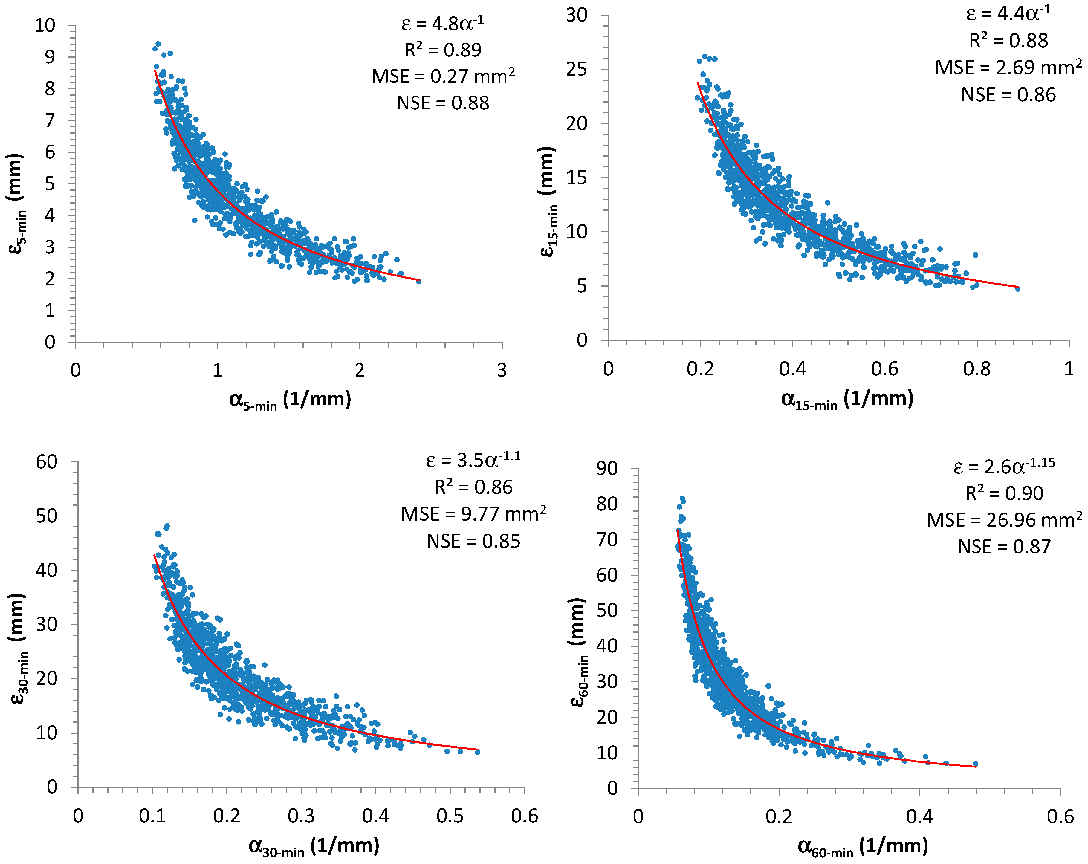
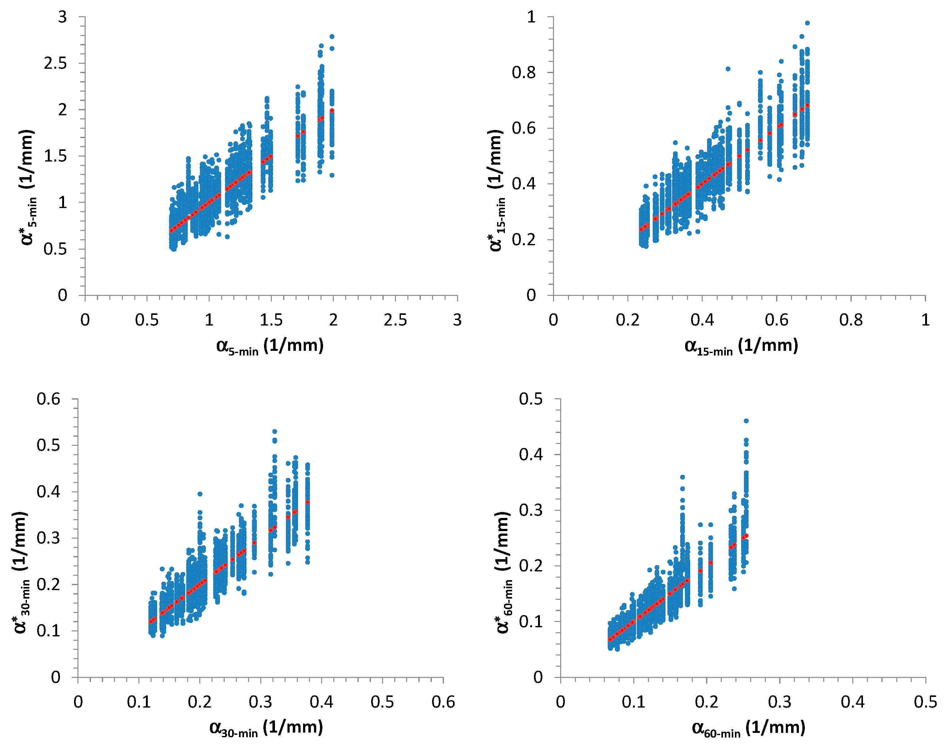
Analyzing the synthetic samples, Figure 2 shows the scatter plots between $\alpha$ and $\epsilon$, which were estimated by using the maximum-likelihood (ML) method [43], for each considered time-resolution (5, 15, 30, and 60 min). From Figure 2 it is clear, as expected, that there is an inverse dependence between these two EV1 parameters (see Equation (9) and impose, for simplicity, a fixed value of $\mu$). Moreover, in Figure 2, the authors also reported the best regression equations representing the relationships between $\epsilon$ and $\alpha$ (expressed in this case as a power formula), estimated for each duration, together with the corresponding values of performance measures, mentioned in Section 2.2. 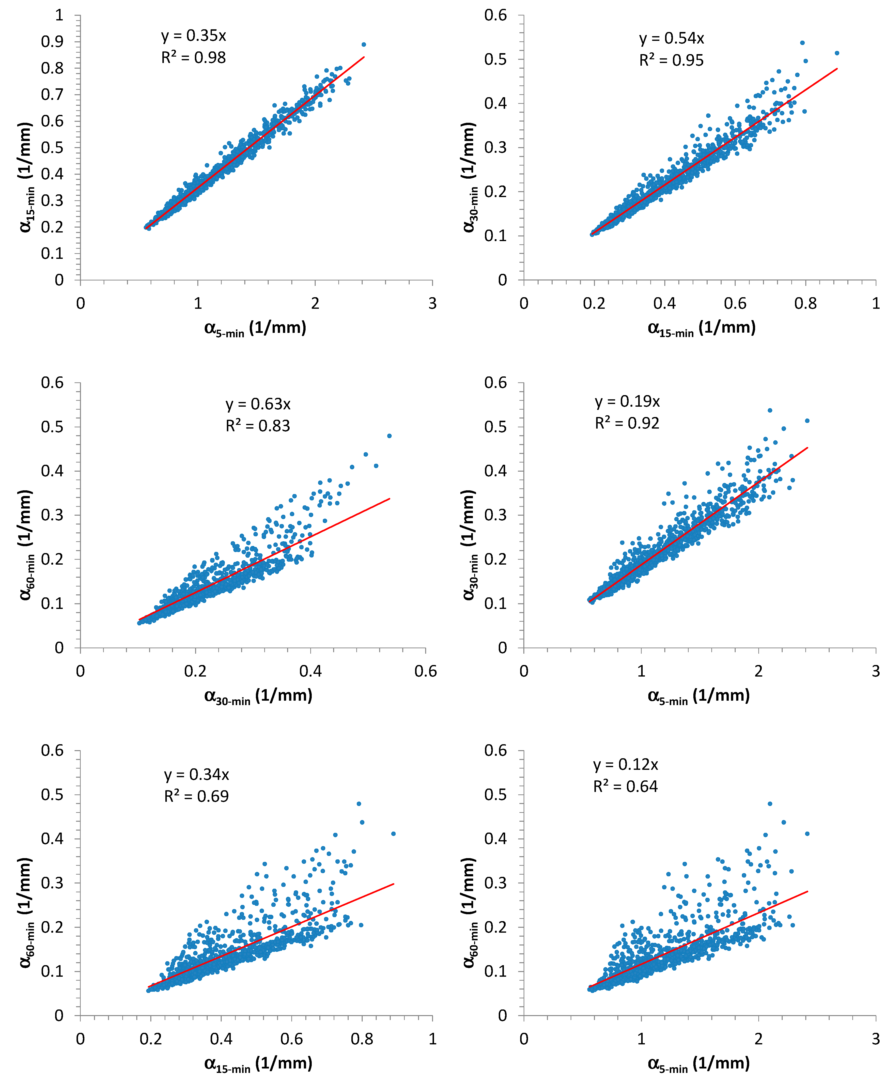Due to the obtained high values for $R^2$ (always greater than or equal to 0.86) and $NSE$ (always greater than or equal to 0.85), i.e., close to 1, the estimated formulas clearly constitute a good fitting. Furthermore, the relationships among the various $\alpha$ parameters are illustrated in Figure 3.

The authors investigated the possible relationships among NSRP and EV1 parameters by mainly focusing on $\alpha$, because $\epsilon$ is strictly connected to $\alpha$, as illustrated in Figure 2.

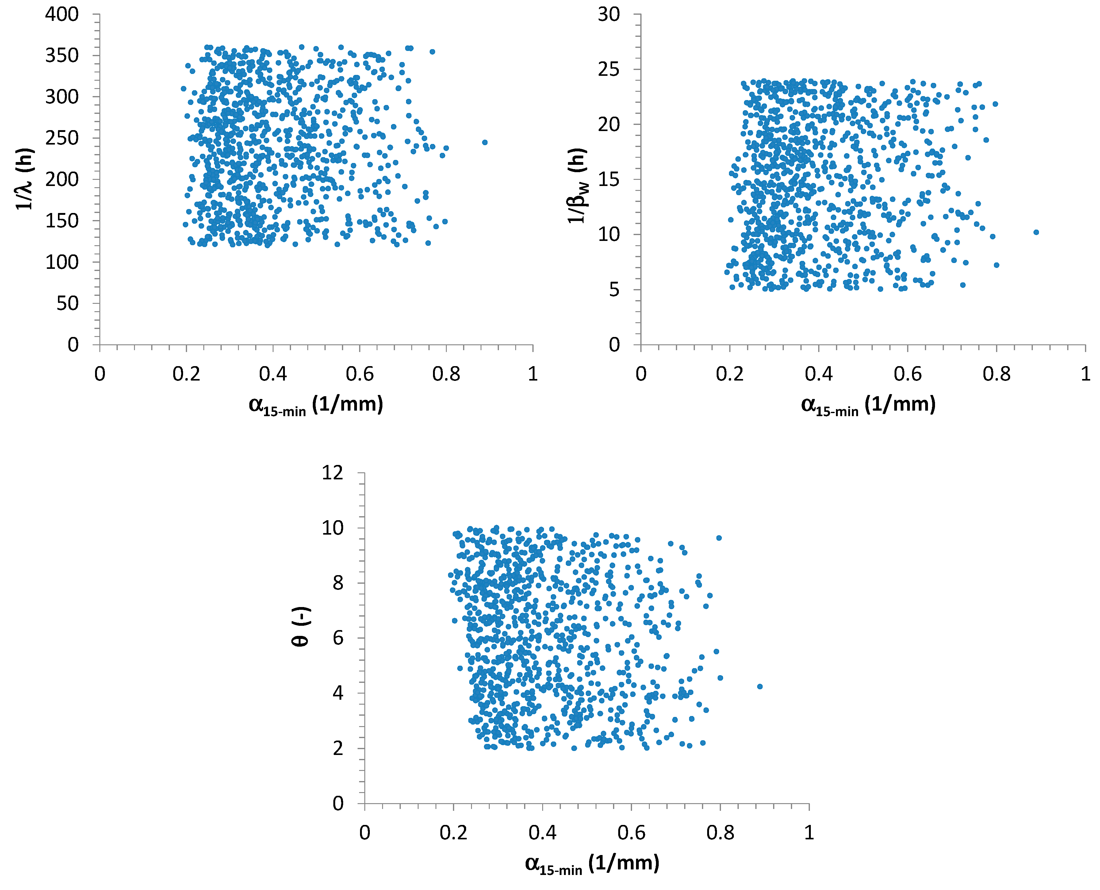
This analysis highlighted that $\lambda$, ${\beta }_W$, and $\theta$ seem to not influence the extreme values distribution at high resolutions. As examples, scatter plots among $\alpha$ estimated from 15-min AMR series and $\lambda$, ${\beta }_W$, $\theta$ are reported in Figure 4.

These results can be justified as follows:

• It is expected that the waiting time between two consecutive storm occurrences could imply effects on monthly and annual scale, but not at finer resolutions (in particular, sub-hourly). In fact, a heavy rainfall event can fully develop itself, without being affected by a large or short waiting time with the previous and the successive storms. Greater values for $1/\lambda$ could determine large dry periods and consequently low aggregated rainfall values only at monthly and yearly scales.
• Similar considerations can be made for $\theta$ and ${\beta }_W$. In fact, the number of bursts (and consequently their occurrences) for each storm could mainly influence the aggregated process (see Equation (7) and Figure 1) at coarser resolutions (from daily or multi-daily), but not at finer scales (hourly and sub-hourly), especially if durations of the pulses are always sub-hourly on average, as assumed in this work (see Table 1).

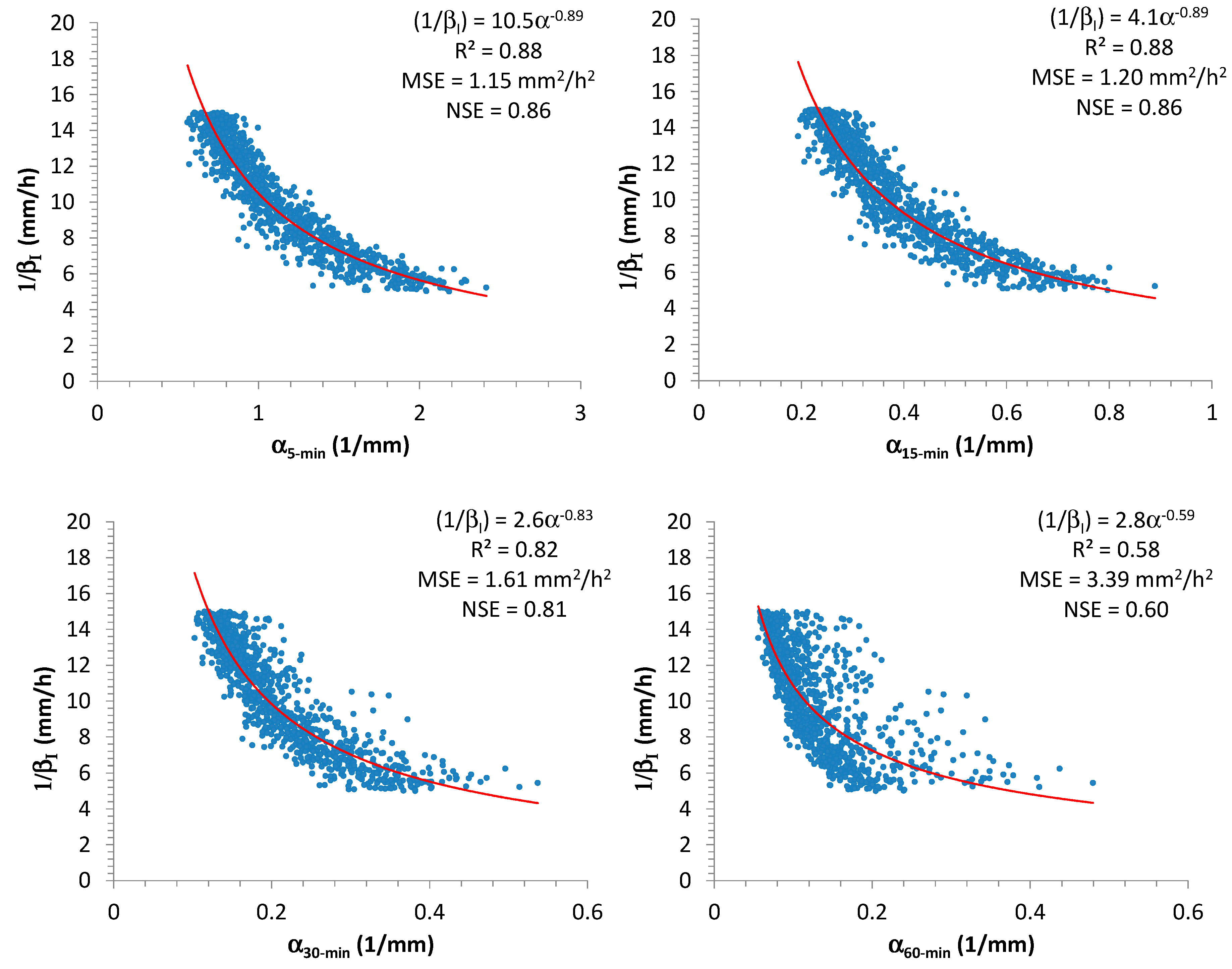
On the contrary, ${\beta }_I$ and ${\beta }_D$ show a more evident influence for EV1 distributions of high-resolution rainfall data.

In particular, the scatter plots in Figure 5 remark a significant interconnection between α and ${\beta }_I$, mainly for 5 and 15 min. Considering that observed 15-min AMR series are more available than 5-min ones in many locations, the authors chose to use the relationship between ${\beta }_I$ and ${\alpha }_{15\min }$ for the successive elaborations:

$$\frac{1}{{\beta }_I}=b_0\cdot {\alpha }_{15\min }^{b_1}.$$

(14)

Minimization of $MSE$ (and simultaneous maximization of $R^2$) and maximization of $NSE$ provided $b_0$ = 4.1, $b_1$ = −0.89, with $MSE$ = 1.2 (mm²/h²), $R^2$ = 0.88, and $NSE$ = 0.86. From Equation (14) it is clear that the authors focused on $1/{\beta }_I$, and this implies that $MSE$ is expressed in mm²/h². In Figure 5, the estimated coefficients for Equation (14), together with the associated values of $MSE$, $R^2$, and $NSE$ are also reported for the other durations. From result analysis, it is evident that adoption of 15-min AMR series produces similar good performances of 5-min AMR series. On the contrary, the use of 60-min AMR series (if it were the unique available data set for a specific site) could not provide a good reconstruction for ${\beta }_I$ ($R^2$ = 0.58 and $NSE$ = 0.60).

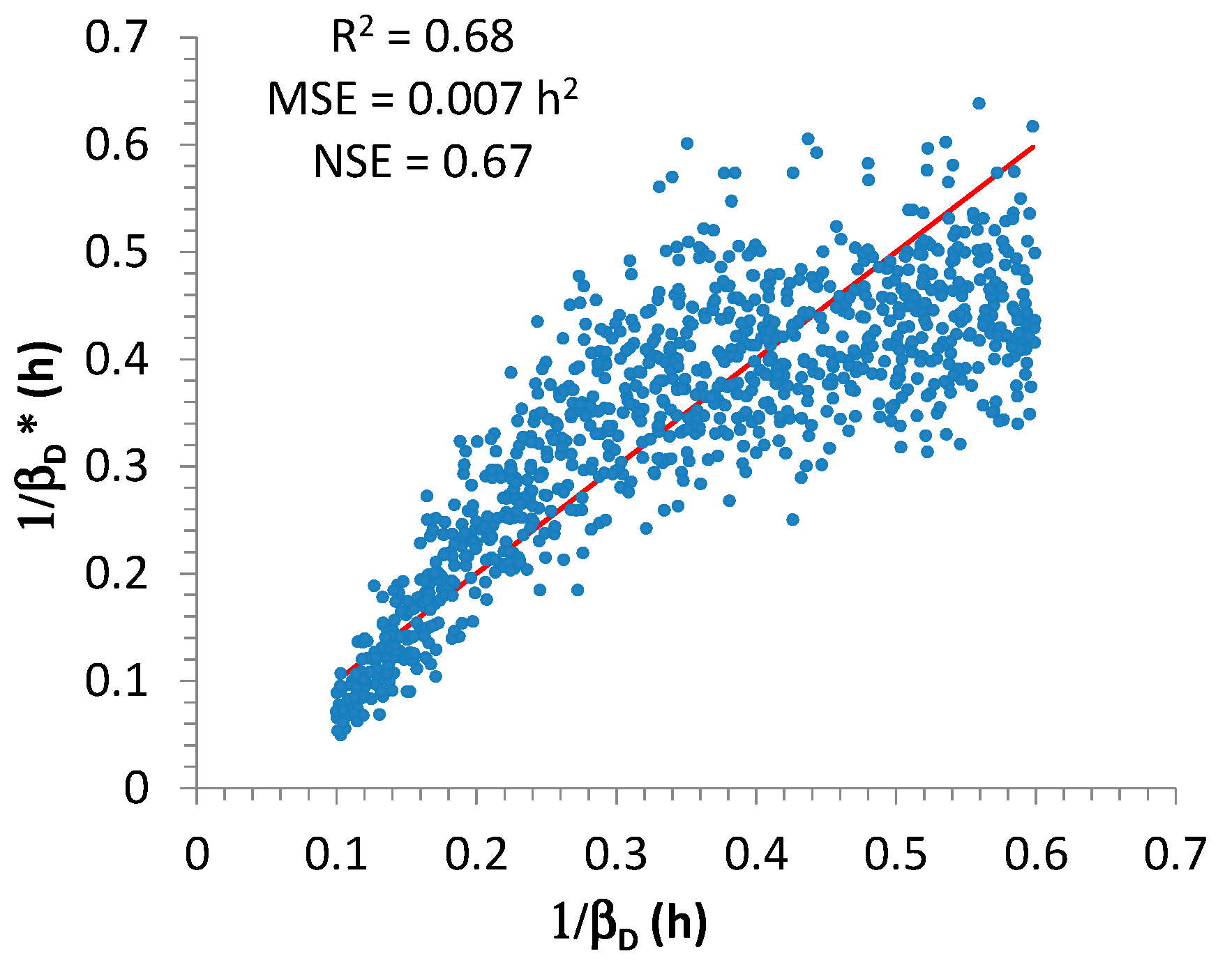
As regards ${\beta }_D$, the best relationship was found by linking with estimates of α for 15 and 60 min (Figure 6):

$$\frac{1}{{\beta }_D}=c_0\cdot {\alpha }_{15\min }^{c_1}\cdot {\alpha }_{60\min }^{c_2},$$

(15)

with $c_0$ = 0.015, $c_1$ = 2.3, $c_2$ = −2.5; the associated values for the performance measures were $MSE$ = 0.007 h², $R^2$ = 0.68, and $NSE$ = 0.67. From Equation (15), it is clear that the authors focused on $1/{\beta }_D$, and this implies that $MSE$ is expressed in h². From a visual analysis of Figure 6, the performance is clearly not comparable with that for ${\beta }_I$, however it was considered as acceptable for the successive elaborations, because the values of $R^2$ and $NSE$ are greater than 0.5 [47].

3.2. Validation

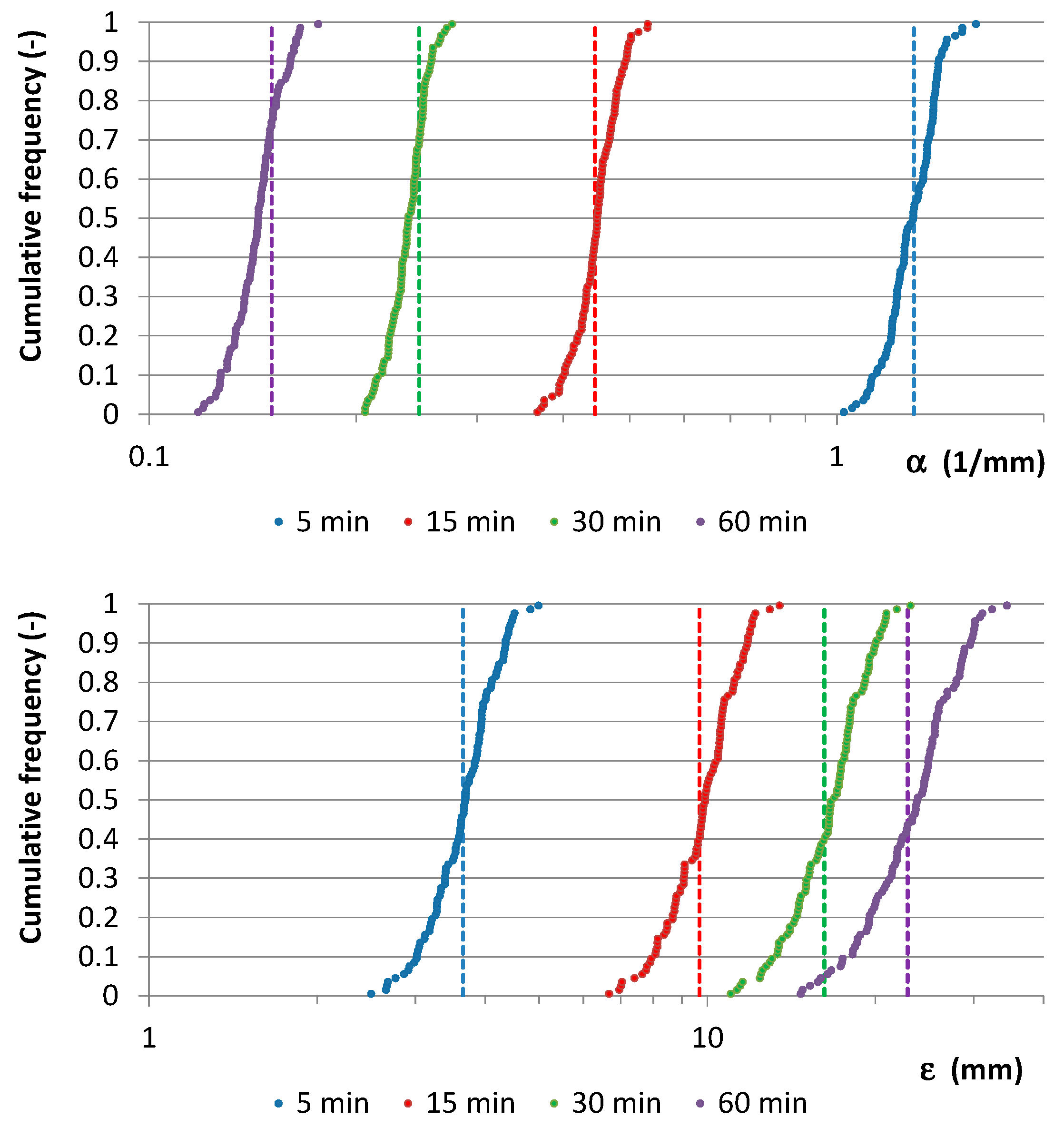
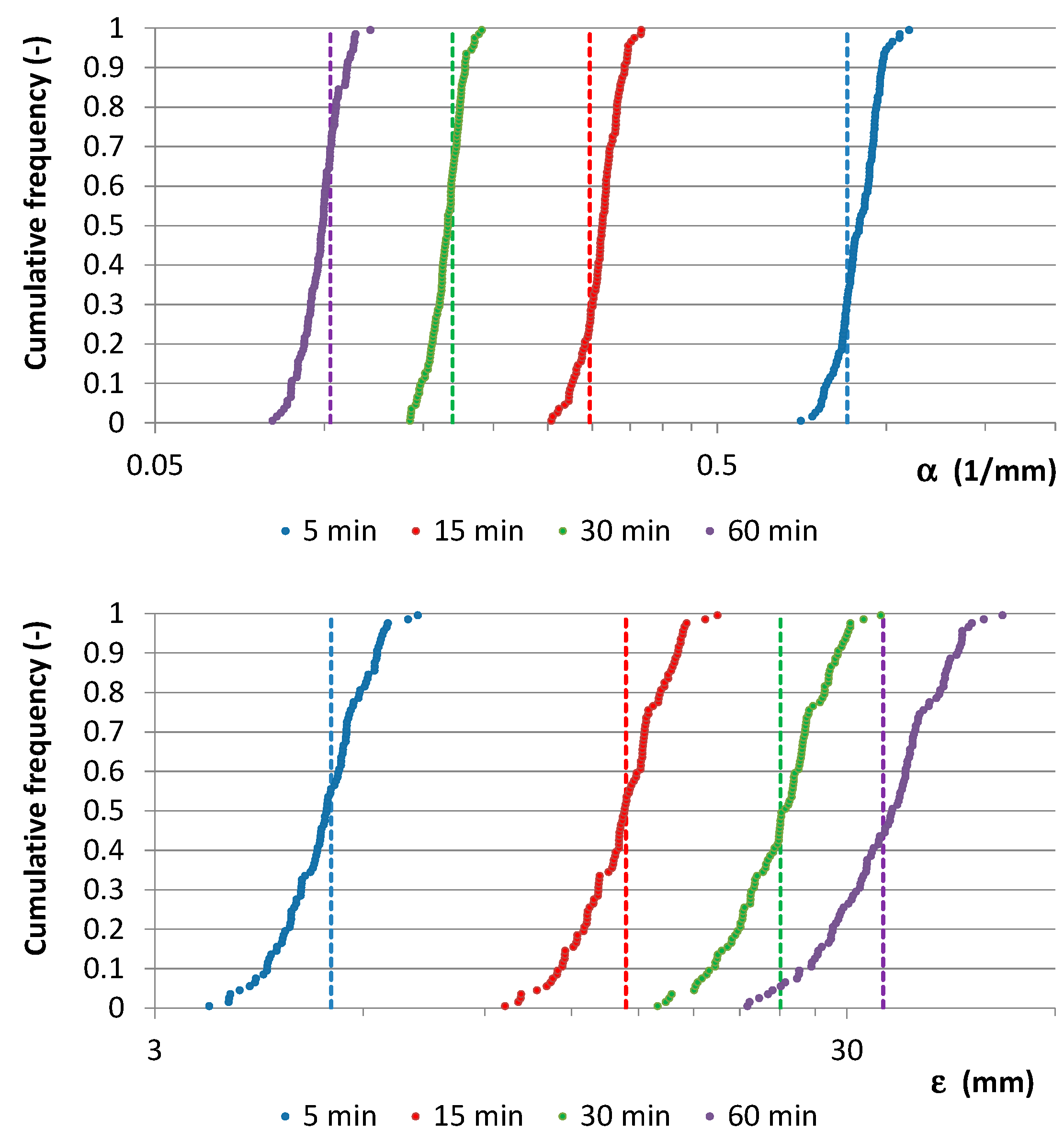
First of all, the authors validated the proposed procedure by focusing on:

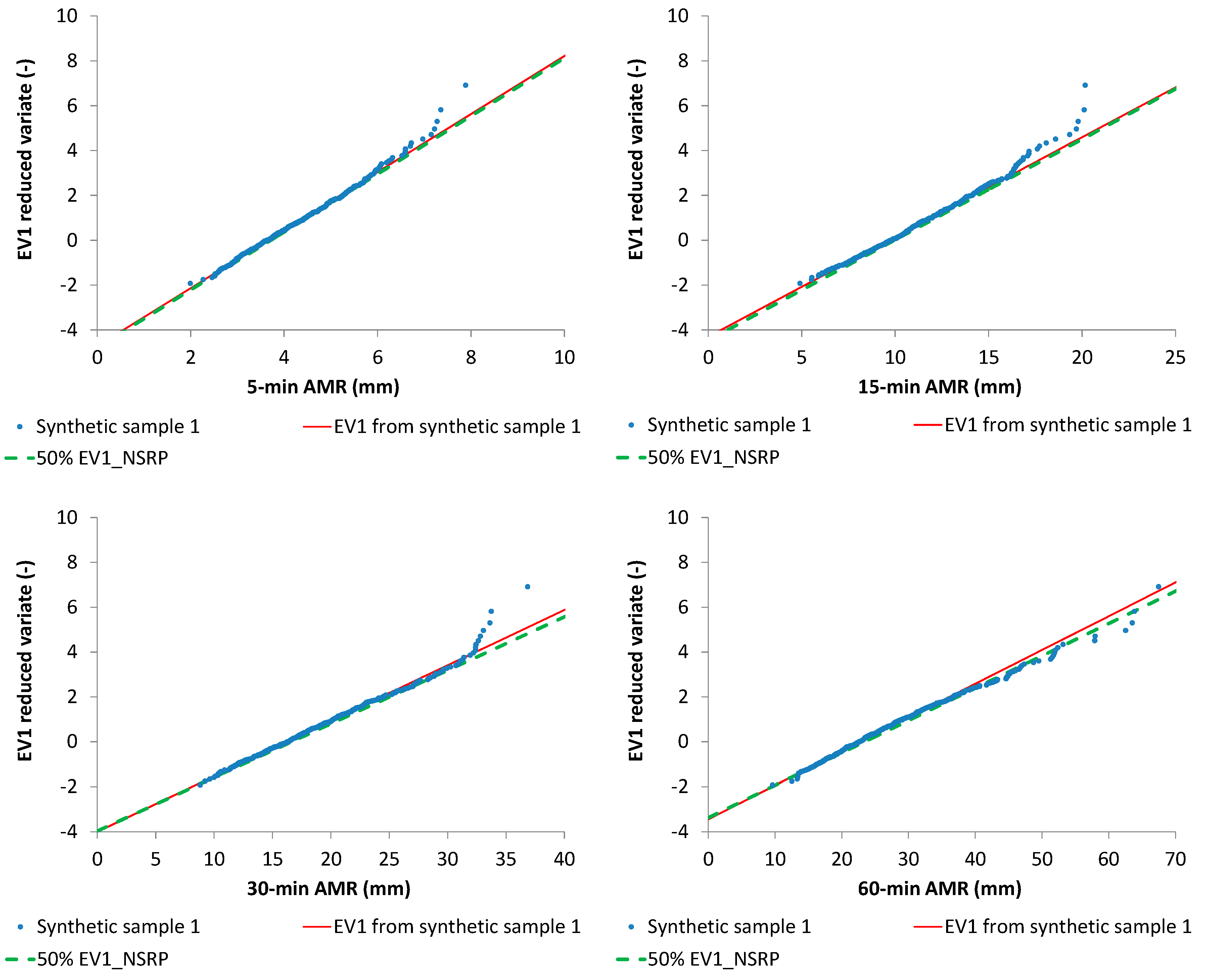
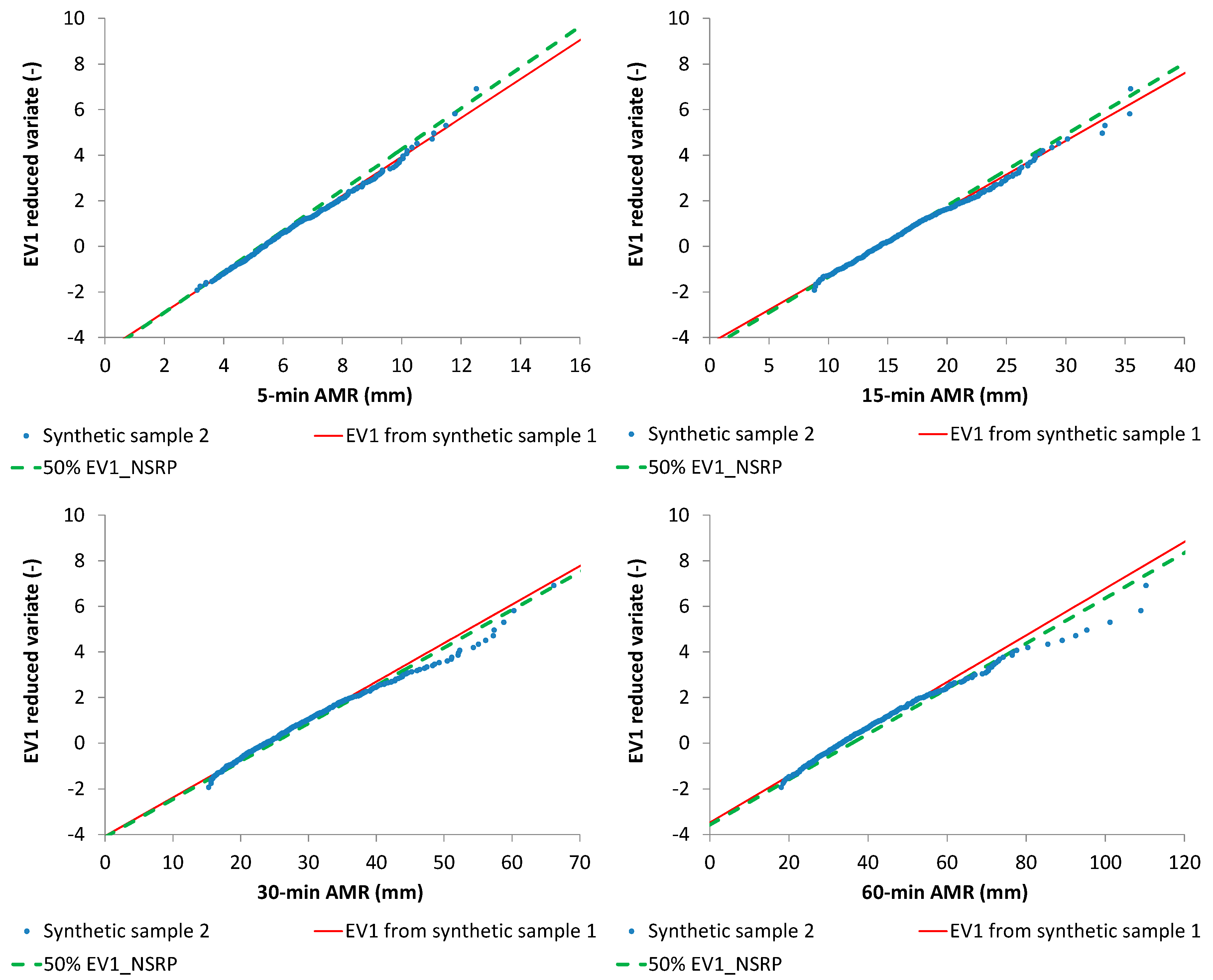
• two 500-year synthetic samples with a resolution of 1 min, generated from NSRP with parameter sets reported in

  Table 2. NSRP parameters for two synthetic samples analyzed in the validation step.

  NSRP Parameter	$\mathbf{1}\mathbf{/}\mathit{\lambda }$ (h)	$\mathit{\theta }$(-)	${\mathbf{1}\mathbf{/}\mathit{\beta }}_{\mathit{W}}$ (h)	${\mathbf{1}\mathbf{/}\mathit{\beta }}_{\mathit{I}}$ (mm/h)	${\mathbf{1}\mathbf{/}\mathit{\beta }}_{\mathit{D}}$ (h)
  Synthetic sample 1	240	6	8	8	0.25
  Synthetic sample 2	240	6	8	12	0.25

  , from which 5, 15, 30, and 60-min AMR series were derived (Figure 7, Figure 8, Figure 9 and Figure 10), and;
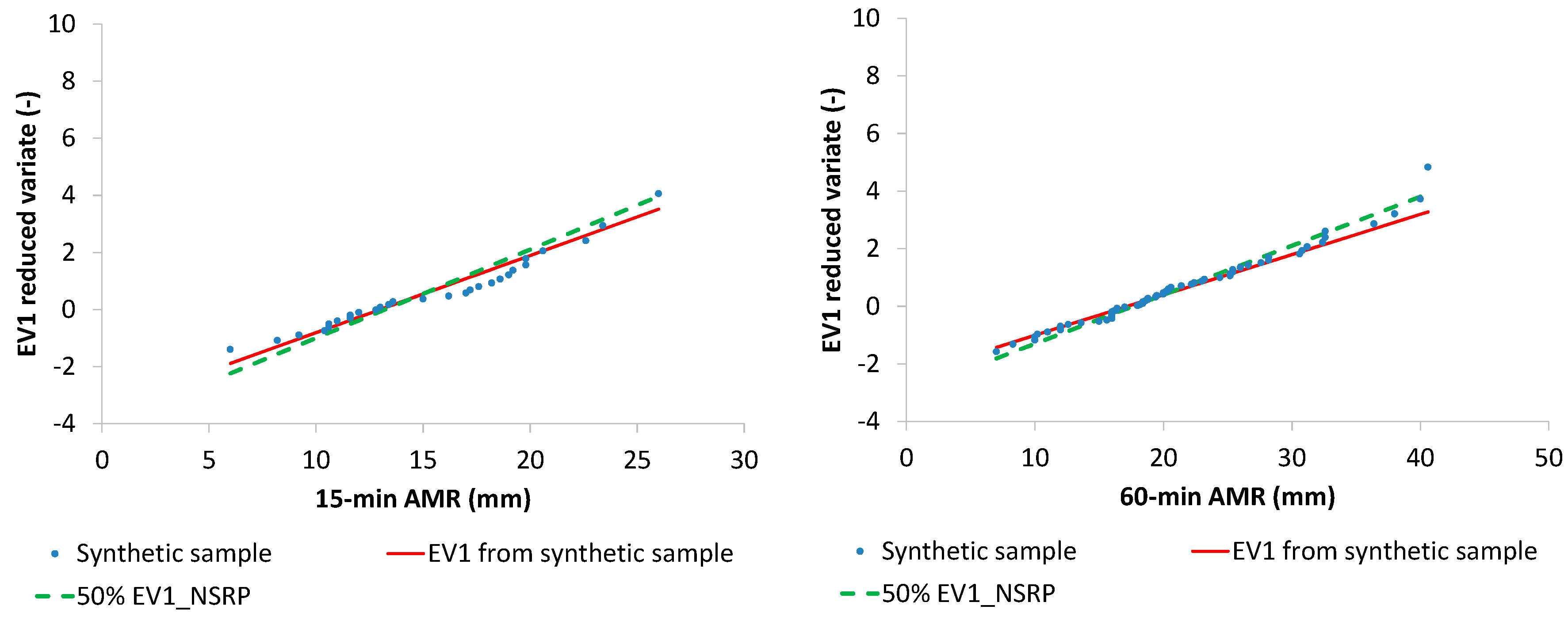
• observed 15-min and 60-min AMR series, related to Cosenza rain gauge (Southern Italy), having a sample size M = 29 years for 15-min AMR and M = 63 years for 60-min AMR, and characterized by a clear EV1 behavior, as shown in EV1 probabilistic plots (Figure 11).

For each (virtual or real) site, as theoretically explained in Section 2.3:

➢

EV1 parameters were estimated with ML technique (see

Table 3. EV1 parameters for two synthetic samples analyzed in the validation step.

	5 min		15 min		30 min		60 min
EV1 Parameter	$\mathit{\alpha }$ (1/mm)	$\mathit{\epsilon }$ (mm)	$\mathit{\alpha }$ (1/mm)	$\mathit{\epsilon }$ (mm)	$\mathit{\alpha }$ (1/mm)	$\mathit{\epsilon }$ (mm)	$\mathit{\alpha }$ (1/mm)	$\mathit{\epsilon }$ (mm)
Synthetic sample 1	1.30	3.65	0.45	9.68	0.25	16.21	0.15	22.85
Synthetic sample 2	0.85	5.40	0.30	14.40	0.17	24.06	0.10	33.85

and

Table 4. EV1 parameters for AMR series of Cosenza rain gauge.

	15 min		60 min
EV1 Parameter	$\mathit{\alpha }$ (1/mm)	$\mathit{\epsilon }$ (mm)	$\mathit{\alpha }$ (1/mm)	$\mathit{\epsilon }$ (mm)
Cosenza rain gauge	0.27	13	0.14	17.2

) for the associated AMR series.

➢

1000 NSRP five-parameter sets were generated, in which $\lambda$, ${\beta }_W$, and $\theta$ vary in a uniform way within the ranges reported in Table 1, while ${\beta }_I$ and ${\beta }_D$ values are always the same, calculated from Equations (14) and (15), by using the estimated $\alpha$ parameters from the previous step (see

Table 5. NSRP parameters for two synthetic samples derived from EV1 parameters in Table 3.

NSRP Parameter	$\mathbf{1}\mathbf{/}\mathit{\lambda }$ (h)	$\mathit{\theta }$ (-)	${\mathbf{1}\mathbf{/}\mathit{\beta }}_{\mathit{W}}$ (h)	${\mathbf{1}\mathbf{/}\mathit{\beta }}_{\mathit{I}}$ (mm/h)	${\mathbf{1}\mathbf{/}\mathit{\beta }}_{\mathit{D}}$ (h)
Synthetic sample 1	[120; 360]	[2; 10]	[5; 24]	8.43	0.26
Synthetic sample 2	[120; 360]	[2; 10]	[5; 24]	12.10	0.27

and

Table 6. NSRP parameters for Cosenza rain gauge derived from EV1 parameters in Table 5.

NSRP Parameter	$\mathbf{1}\mathbf{/}\mathit{\lambda }$ (h)	$\mathit{\theta }$ (-)	${\mathbf{1}\mathbf{/}\mathit{\beta }}_{\mathit{W}}$ (h)	${\mathbf{1}\mathbf{/}\mathit{\beta }}_{\mathit{I}}$ (mm/h)	${\mathbf{1}\mathbf{/}\mathit{\beta }}_{\mathit{D}}$ (h)
Cosenza rain gauge	[120; 360]	[2; 10]	[5; 24]	13.15	0.10

).

➢

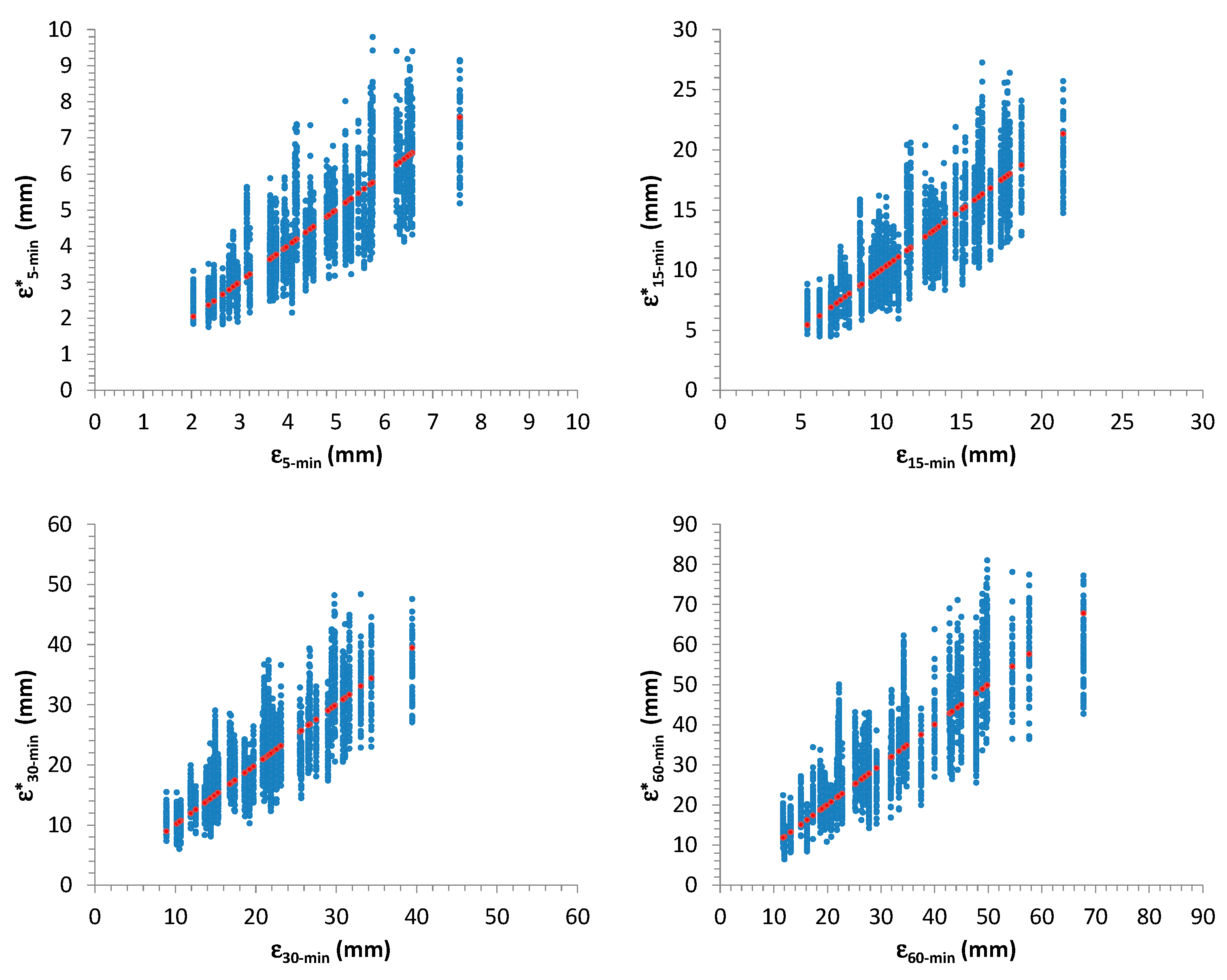
For each generated NSRP five-parameter set, a 500-year continuous 1 min data series was reproduced, from which the associated 5, 15, 30, and 60-min AMR series were extracted, together with the correspondent EV1 parameter estimations.

➢

From the previous step, frequency distributions for $\alpha$, $\epsilon$ were obtained and compared with the ML estimates related to the specific (virtual or real) starting data series (Figure 7 and Figure 8). Comparisons were also carried out in EV1 probabilistic plots (Figure 9 and Figure 10), among starting AMR series, their EV1 theoretical curves, and EV1 curves associated with (i) median values for $\alpha$ and (ii) $\epsilon$ values which were calculated with the relationships reported in Figure 2.

From Figure 7 and Figure 8, it is clear that the starting value for $\epsilon$ is about the median value of the cumulative frequency distribution for each analyzed duration, while the starting value for $\alpha$ is always inside the interquartile range. Moreover, EV1 probabilistic plots (Figure 9 and Figure 10) show that median EV1 curves from NSRP generation and EV1 theoretical curves from synthetic AMR series perform equally well.

Similar results were obtained for Cosenza rain gauge. In detail, median EV1 curves from NSRP generation reconstruct in an acceptable way the sample data, with respect to EV1 theoretical curves, which were directly estimated from the observed AMR series (Figure 11).

The performance of EV1 distributions, obtained (i) directly with ML parameter estimation from synthetic samples and Cosenza data set and (ii) from NSRP generation, were analyzed by comparison with the sample frequency values, also in this case in terms of $MSE$, $R^2$, and $NSE$ (see

Table 7. Evaluation of EV1 distributions for synthetic samples and Cosenza data series.

		50% EV1_NSRP				ML Parameter Estimation from Data
	Performance Measures	5 min	15 min	0 min	60 min	5 min	15 min	30 min	60 min
Synthetic sample 1	$MSE$	0.017	0.042	0.037	0.019	0.010	0.024	0.018	0.018
	$R^2$	0.99	0.99	0.99	0.99	0.99	0.99	0.99	0.99
	$NSE$	0.99	0.97	0.98	0.99	0.99	0.99	0.99	0.99
Synthetic sample 2	$MSE$	0.041	0.023	0.036	0.069	0.006	0.008	0.033	0.018
	$R^2$	0.99	0.99	0.99	0.99	0.99	0.99	0.99	0.99
	$NSE$	0.98	0.99	0.98	0.96	0.99	0.99	0.98	0.99
Cosenza data series	$MSE$		0.143		0.041		0.090		0.049
	$R^2$		0.96		0.98		0.96		0.98
	$NSE$		0.91		0.96		0.94		0.98

). The obtained results showed that reconstruction of extreme events from the proposed calibration of a NSRP model provides similar performances with respect to the theoretical frequency distributions which were directly estimated from AMR data: $R^2$ and $NSE$ always assumed values greater than 0.9.

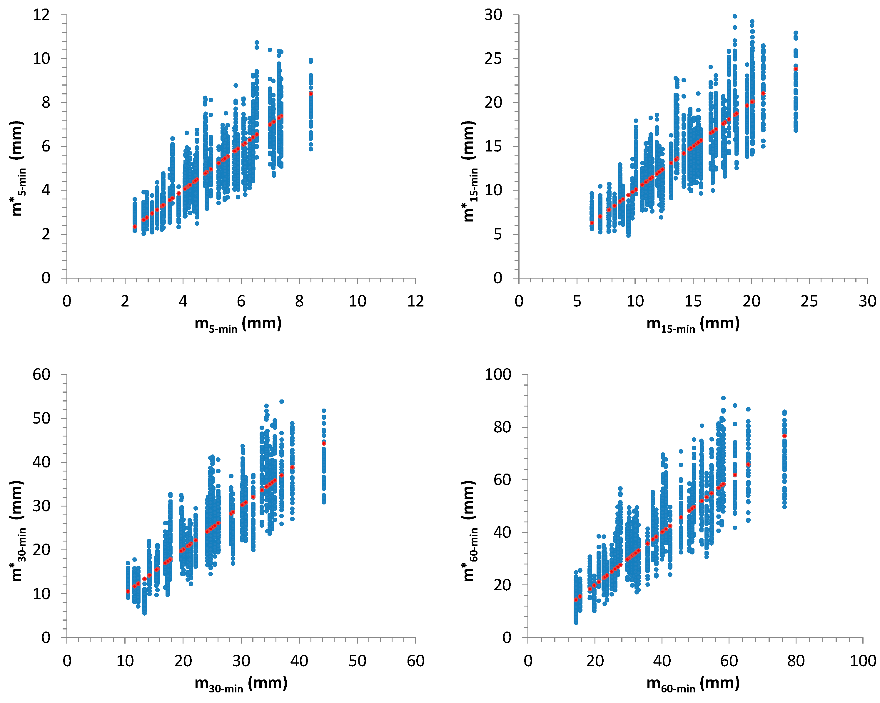
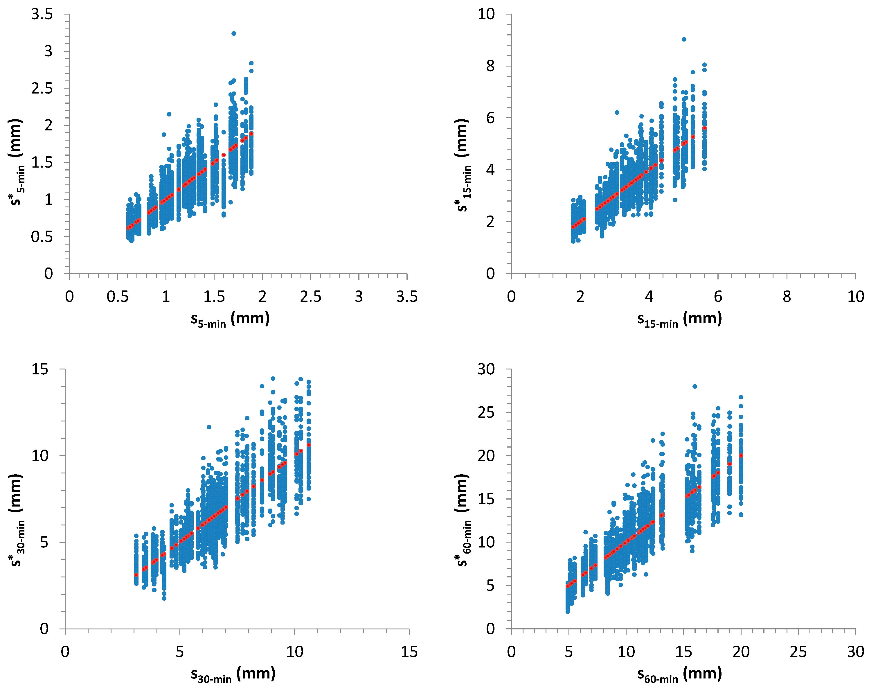
As another check, the authors repeated the validation for a further 50 synthetic samples, generated from 50 NSRP parameter sets which were randomly chosen from the ranges in Table 1.

Figure 12, Figure 13, Figure 14 and Figure 15 summarize the outcomes: starting values for $\alpha$, $\epsilon$ and for sample mean, m, and standard deviation, s, related to 50 AMR series were compared with the associated distributions derived from the further 1000 generated samples for each considered one. In many cases, the starting values are very close to the median of the distributions.

4. Discussion

The overall obtained results are highly promising, as they make possible the use of only AMR series (having very long sample sizes in many locations) for defining some features of the continuous process (for which sample sizes are shorter or absent for many sites). This is clearly an important aspect: unlike all the previous works, also mentioned in Section 1, the proposed methodology does not consider the usually limited continuous data series at high resolution for a SRG calibration, but uses the longer AMR series, and this allows for a good reconstruction of extreme events, without applying any change in model structure for a SRG (as in [9,30,31,32]) or introducing disaggregation techniques (as in [33,34,35,36]), censor values [38], or increasing in general the number of parameters.

In this work, the authors investigated the crucial role of sub-hourly AMR series, which can be considered as correlated with the statistical properties of intensity and duration for the rectangular pulses. Moreover, this research revalued the rectangular shape, as it was judged in many previous papers as “unsuitable for fine-scale data” [9] due to underestimation of extreme values at fine temporal scales.

It is clear that the proposed approach is highly flexible, and then it can be applied for other kinds of SRGs, in which: (i) the probability distributions are different from those adopted in Equations (1)–(5) and/or (ii) the pulses are hypothesized to have another shape, different from rectangular [9,30,31,32] and/or (iii) other probability distributions are adopted for AMR series.

Future interesting developments in this research can regard the study of possible importance for other data series (as examples, daily and multi-daily AMRs, monthly and annual rainfall data), of greater length than continuous data at fine scales, in order to better explain other significant features of continuous process, such as those represented by $\lambda$, ${\beta }_W$, and $\theta$ in a NRSP model, which were considered here as irrelevant for sub-hourly AMR series.

In fact, as already highlighted in Section 3.1, it is expected that inter-arrivals between two consecutive storms, and the associated number of bursts with their temporal occurrences, could mainly influence aggregated rainfall heights at coarser resolutions (e.g., multi-daily, monthly, and yearly), while short-duration heavy rainfall events should not depend on these features. Moreover, seasonality is another important aspect to take into account, and, in particular, the research should focus on which NRSP parameters need of assumptions of a cyclostationary nature. This work remarked that seasonality is not essential for intensity and duration of the rectangular pulses, but it could be necessary for other parameters, mainly for a good modeling of dry/wet periods, not investigated here.

5. Conclusions

This described work constitutes the first step of an interesting research, aimed to investigate the possibility of a good calibration for models such as the NSRP, suitable for the generation of continuous high-resolution rainfall series, by using only data from annual maximum rainfall (AMR) series at fine scales, which are usually longer than continuous sub-hourly series, or they are the unique available data set for many locations.

The obtained results highlighted the crucial role of high-resolution extreme value distributions as important signatures for defining the statistical properties of intensity and duration for rectangular pulses, without considering continuous high-resolution rainfall data.

Future works will refer to the investigation of other possible signatures, deriving from further data series of greater length and available for many locations, such as multi-hourly and daily/multi-daily AMRs, or monthly and annual aggregated rainfall heights, in order to realize a comprehensive framework for the calibration of SRGs, in which it would be possible to estimate other important parameters (such as $\lambda$, ${\beta }_W$, and $\theta$ in NSRP), also taking into account the seasonality, without the need to use continuous time series at finest scales, whose sample sizes are still short for many sites.

Moreover, in the context of climate change, the discussed results and the flexible structure of a NSRP model can allow for investigation of potential trends into the continuous process at fine scales by analyzing/checking possible non-stationary behaviors in AMRs and in other longer series.

Obviously, improvements in the reconstruction of continuous rainfall series can also benefit the modeling of all those quantities which are connected with a pluviometric input, at hydrological space–time scales, such as streamflow time series in small basins and occurrences of shallow landslides.