Coupled Stress-Dependent Groundwater Flow-Deformation Model to Predict Land Subsidence in Basins with Highly Compressible Deposits

Abstract

In this study, a stress-dependent groundwater model, MODFLOW-SD, has been developed and coupled with the nonlinear subsidence model, NDIS, to predict vertical deformation occurring in basins with highly compressible deposits. The MODFLOW-SD is a modified version of MODFLOW (the USGS Modular Three-Dimensional Groundwater Flow Model) with two new packages, NONK and NONS, to update hydraulic conductivity and skeletal specific storage due to change in effective stress. The NDIS package was developed based on Darcy–Gersevanov Law and bulk flux to model land subsidence. Results of sample simulations run for a conceptual model showed that hydraulic heads calculated by MODFLOW significantly overestimated for confining units and slightly underestimated for aquifer ones. Moreover, it showed that applied stress due to pumping changed initially homogeneous layers to be heterogeneous ones. Comparison of vertical deformations calculated by NDIS and MODFLOW-SUB showed that neglecting horizontal strain and stress-dependency of aquifer parameters can overestimate future subsidence. Furthermore, compared to the SUB (Subsidence and Aquifer-System Compaction) package, NDIS is more likely to provide a more accurate compaction model for a complex aquifer system with vertically variable compression ($C_c$), recompression $\left(C_r\right)$, and hydraulic conductivity change ($C_k$) indices.

1. Introduction

Groundwater models have been used to understand the mechanics of an aquifer system and to predict the system response to future extraction scenarios. Coupling these models with associated processes, including solute transport and land movement, is a common approach to model the resulting geohazards.

Land movements include vertical and horizontal components (land subsidence and fissures), causing damages to infrastructures such as bridges and highways [1]. Land subsidence can be gradual settling or the sudden sinking of discrete segments of the ground surface [2]. Land subsidence associated with groundwater extraction is the outcome of the compaction of susceptible geologic layers or units caused by long-term groundwater extraction and under a transient flow condition. In the coastal region, land subsidence combined with other natural disasters, such as sea level rise due to global warming and extreme weather such as hurricanes, will result in serious environmental and economic problems. For example, in 2005 the occurrence of Hurricane Katrina created a natural disaster by flooding the subsiding coastal city, New Orleans, and caused over 1600 fatalities and $30 billion in direct economic losses in southern Louisiana [3]. The latest flood caused by Hurricane Harvey (2017) in the Houston-Galveston region was regarded as one of the costliest disasters in the U.S. history, with damages exceeding $100 billion [4]. Unfortunately, other than being vulnerable to natural hazards like hurricanes, many coastal cities also experience significant land subsidence and sea level rise which both exacerbate the urban floods [5].

Regional land subsidence accompanying groundwater extraction and its severe environmental consequences were reported in different locations around the world, e.g., Mexico City, Mexico [6], Beijing, China [7], Houston-Galveston, Texas, USA [8], and Santa Clara Valley, California, USA [9]. Recent worldwide measured subsidence rates for major cities that experienced substantial land subsidence showed subsidence as small as several mm/year to 38 cm/year [2,10,11].

Excessive groundwater pumping declines artesian head and pore pressure in an aquifer system. Under the assumption of constant total stress, this decline causes pore water pressure to decrease and effective stress to increase. The increase in effective stress results in the compaction of compressible units within an aquifer system, including aquitards and interbeds clay lenses. As long as the effective stress remains less than the pre-consolidation stress, compaction is elastic and recoverable [12]. Increases in effective stress that exceeds pre-consolidation stress result in inelastic compaction. Inelastic compaction causes permanent deformation that cannot be recovered after unloading and diminishes the storage capacity of the aquifer system. The cumulative deformation of all compressible units is emerged on the earth surface as the land subsidence and fissures.

MODFLOW, the USGS Modular Three-Dimensional Groundwater Flow Model [13], is the well-known standard model used worldwide. MODFLOW consists of a main program and different independent modules. Different compaction packages, e.g., Interbed Storage (IBS1) [14] and Subsidence and Aquifer-System Compaction (SUB) [15], have been developed to model land subsidence and compaction of deformable layers based on hydraulic head distribution calculated by MODFLOW. These packages can produce vertical land movement models using constant aquifer parameters, including hydraulic conductivity and specific storage [15]. Though few compaction packages, e.g., SUB-WT (the Subsidence and Aquifer-System Compaction Package for Water-Table Aquifers) [16], have been developed to consider stress-dependent specific storage, a nonlinear groundwater flow equation including stress-dependent hydraulic conductivity and specific storage has not been considered. Some studies have shown that these packages might overestimate future subsidence [14,16,17,18]. This is firstly because the volume strain is entirely converted to vertical strain and, secondly, future reductions in soils parameters, including conductivity and skeletal storage, due to increase in effective stress were not accounted for.

DIS, the aquifer movement package, was developed by Zhang [19] on the basis of Darcy–Gersevanov Law and bulk flux. This package has been employed to simulate three-dimensional land subsidence using constant aquifer parameters and linear stress-strain relation. For highly compressible soils, soil properties including permeability and compressibility vary significantly with changes in effective stress. This fact needs to be considered and appropriately implemented in the modeling process to simulate groundwater flow and land subsidence more accurately [20,21,22,23]. Li and Ding improved the DIS package and introduced stress-dependent specific storage [24]. In this study, a three-dimensional stress-dependent groundwater flow model has been developed and coupled with Darcy–Gersevanov Law and bulk flux to model vertical land subsidence.

2. Methodology

2.1. Groundwater Flow Equation

The governing equation for three-dimensional groundwater flow through a saturated anisotropic porous material in a Cartesian coordinate system can be expressed as follows [13]:

$$\nabla ·\left(\mathrm{K}\nabla h\right)-W=S_s\frac{\partial h}{\partial t}$$

(1)

where h is the hydraulic head; K is the hydraulic conductivity, a second order tensor; W is the volumetric flux per unit volume that represents sources and/or sinks of water; $S_s$ is the specific storage; t is time.

It is conventionally assumed that K and $S_s$ are constant for geologic layers in an aquifer system. This assumption implies that Equation (1) is a linear partial differential equation. A general form of groundwater flow equation can be expressed by rewriting Equation (1) for highly compressible and saturated sedimentary materials, as follows:

$$\nabla ·\left(K_h\nabla h\right)-W=S_s{}_h\frac{\partial h}{\partial t}$$

(2)

where $K_h$ and $S_s{}_h$ are hydraulic conductivity and specific storage, and the both are functions of hydraulic head or effective stress. Equation (2) is a nonlinear partial differential equation which can be solved using iterative methods via numerical modeling.

2.2. Aquifer Movement

Any groundwater recharge or discharge will result in generating or changing the existing groundwater flow regime in an aquifer system. As Darcy’s law, a basic relation describing flow of fluid through porous media, assumes the aquifer frame is non-deformable, the Darcy–Gersevanov Law, a generalization of Darcy’s law, can be invoked in Equation (3) to describe the pore water flow through permeable, deformable, and saturated porous media within the aquifer system, as follows [25,26]:

$$\overrightarrow{q}=n\left({\overrightarrow{v}}_w-{\overrightarrow{v}}_s\right)$$

(3)

where $\overrightarrow{q}$ is the specific discharge, n is the porosity, ${\overrightarrow{v}}_w$ and ${\overrightarrow{v}}_s$ are the velocity of water and velocity of solid grains, respectively, and the subscripts w and s denote pore water and soil particles, respectively. Helm [27] gave the definition of bulk flux ${\overrightarrow{q}}_b$ through permeable, deformable, and saturated porous materials based on the volume fraction as below:

$${\overrightarrow{q}}_b=\left(1-n\right){\overrightarrow{v}}_s+n{\overrightarrow{v}}_w$$

(4a)

which yields the following alternative relation [19]:

$${\overrightarrow{q}}_b=\overrightarrow{q}+{\overrightarrow{v}}_s$$

(4b)

The bulk flow will never change with time for unchanging boundary conditions within a stress period. As time progresses, the transient flow, $\overrightarrow{q}$, approaches the bulk flow and the velocity of the solids tends with time towards zero [28]. For constant discharge or recharge rates and under assumption of reaching equilibrium with no aquifer movement at $t=t_{st}$, Equation (4b) can be rewritten as [21]:

$${\overrightarrow{v}}_s={\overrightarrow{q}}_{st}-\overrightarrow{q}$$

(5)

The subscript st denotes steady state condition. Equation (5) implies that at each spatial location in the aquifer system, aquifer sedimentary materials move with the velocity equal to the difference between specific discharges of steady flow and transient flow at time, t, in that location. The concept of the potential function for irrotational incompressible bulk flow can be utilized to express Equation (5) in the form of a hydraulic head, as follows [28]:

$${\overrightarrow{v}}_s=-K\nabla \left(h_{st}-h\right)$$

(6)

where $h_{st}$ and h are the potential functions or heads for steady and transient flow. Equation (6) implies that the difference of $h_{st}$ and h serves the potential driving aquifer’s movement. For given initial and boundary conditions, Equation (2) can be solved for steady and transient flows to find $h_{st}$ and h needed in Equation (6). In addition, the field of aquifer displacement, ${\overrightarrow{u}}_s,$ can be determined by integrating velocity field of solids ${\overrightarrow{v}}_s$ over time, as follows:

$${\overrightarrow{u}}_s={\displaystyle \int }{\overrightarrow{v}}_{s}dt$$

(7)

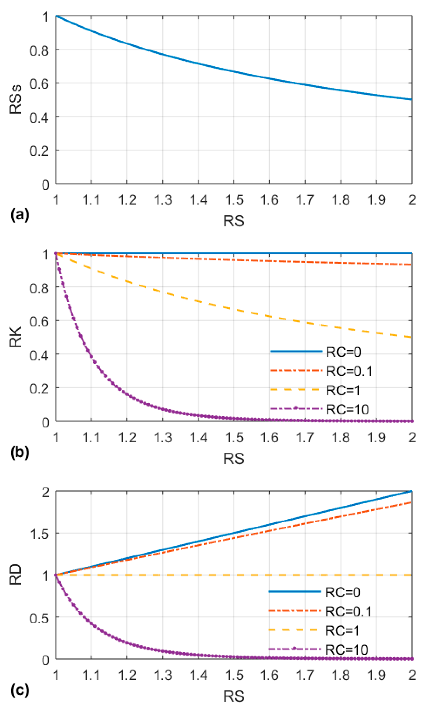
2.3. Aquifer System with Stress-Dependent Parameters

In groundwater modeling, the stress-strain relation in an aquifer system is usually assumed to be linear, which consequently results in employment of constant hydraulic conductivity and specific storage. Based on consolidation lab experiments for cohesive soils, change in the void ratio ($\Delta e$) with respect to change in effective volumetric stress can be expressed as follows [29]:

$$\Delta e=e_0-e=C\log ({\sigma }_v^{\prime }/{\sigma }_{v0}^{\prime })$$

(8)

where $e_0$ and e are initial and current void ratios, $C$ is a dimensionless index (C > 0), and ${\sigma }_{v0}^{\prime }$ and ${\sigma }_v^{\prime }$ are initial and current effective volumetric stresses. Considering the stress history of the soil deposit, a piecewise function can be written to separate elastic and inelastic compactions of soils as follows:

$$\Delta e=\{\begin{array}{c}{C}_r\log ({\sigma }_v^{\prime }/{\sigma }_{v0}^{\prime }){\sigma }_v^{\prime }\le {\sigma }_p^{\prime }\\ C_c\log ({\sigma }_v^{\prime }/{\sigma }_p^{\prime }){\sigma }_v^{\prime }>{\sigma }_p^{\prime }\end{array},$$

(9)

where ${\sigma }_p^{\prime }$ is effective pre-consolidation stress. The values $C_r$ and $C_c$ are recompression and compression indices, respectively, where $C_r\ll C_c$.

The stress-strain relation in a form of an exponential function can be derived using Equation (8) as follows:

$${\sigma }_v^{\prime }={\sigma }_{v0}^{\prime }{10}^{\left(1+e_0\right){\epsilon }_v/C}$$

(10)

where ${\epsilon }_v=\Delta e/\left(1+e_0\right)$ is the volumetric strain and C can be either $C_r$ when ${\sigma }_v^{\prime }\le {\sigma }_p^{\prime }\mathrm{or}{C}_c$ when ${\sigma }_v^{\prime }>{\sigma }_p^{\prime }$. From Equation (10), the apparent nonlinear elastic modulus can be found to be $E=({\sigma }_{v0}^{\prime }/{\epsilon }_v){10}^{\left(1+e_0\right){\epsilon }_v/C}$.

The specific storage for soil with stress-strain behavior in the form of Equation (10) can be expressed as follows [24]:

$$S_s\left({\sigma }_v^{\prime }\right)=\alpha {\gamma }_w=S_{s0}\frac{{\sigma }_{v0}^{\prime }}{{\sigma }_v^{\prime }}$$

(11)

where $S_s\left({\sigma }_v^{\prime }\right)$ is the stress-dependent specific storage, $S_{s0}$ is the initial specific storage, $\alpha$ is the compressibility of soil skeletal, and ${\gamma }_w$ is unit weight of water. In this equation, the compressibility of water is assumed to be negligible. Since initial specific storage, $S_{s0}$, is a function of compressibility of the soil and compressibility itself is a function of C, Equation (11) can be rewritten for elastic and inelastic compactions as the following:

$$S_s\left({\sigma }_v^{\prime }\right)=\{\begin{array}{c}{S}_{ske0}\frac{{\sigma }_{v0}^{\prime }}{{\sigma }_v^{\prime }}{\sigma }_v^{\prime }\le {\sigma }_p^{\prime }\\ S_{skv0}\frac{{\sigma }_{v0}^{\prime }}{{\sigma }_v^{\prime }}{\sigma }_v^{\prime }>{\sigma }_p^{\prime }\end{array}$$

(12)

where $S_{ske0}$ and $S_{skv0}$ are initial elastic and inelastic skeletal specific storage coefficients, respectively, where $S_{ske0}\ll S_{skv0}$. Equation (12) indicates that an increase in effective stress due to groundwater withdrawal (i.e., ${\sigma }_v^{\prime }>{\sigma }_{v0}^{\prime }$) causes a decrease in the specific storage for both elastic and inelastic compactions. From Equation (12), one may conclude that the compaction or deformation will be likely overestimated when using a constant $S_s$ versus a reducing $S_s\left({\sigma }_v^{\prime }\right)$ after the pump turns on. The former assumes material linearity and is larger than the latter, $S_s\left({\sigma }_v^{\prime }\right)$, describing material nonlinearity, in particular, for strain-hardening materials.

For many types of sediment, it has been shown that the curve of hydraulic conductivity versus void ratio is a nonlinear curve. The relation between change in void ratio and change in hydraulic conductivity is defined as follows [30]:

$$\Delta e=-C_k\log (K/K_0)$$

(13)

where $C_k$ is the hydraulic conductivity change index and $K_0$ and K are initial and current values of hydraulic conductivity, respectively. Combining Equations (10) and (13) will result in a general relation between hydraulic conductivity and effective volumetric stress, as follows:

$$K=K_0{\left(\frac{{\sigma }_{v0}^{\prime }}{{\sigma }_v^{\prime }}\right)}^{C/C_k}$$

(14)

As Equation (14) indicates, the hydraulic conductivity of sedimentary materials is a power function of effective volume stress. It is interesting to notice that for a special case, $C=C_k$, Equation (14) reduces to a rational function $K{\sigma }_v^{\prime }=K_0{\sigma }_{v0}^{\prime }=constan$, which suggests that hydraulic conductivity has a reciprocal relation with hydraulic head, namely $K\propto 1/h\left(t\right)$ at a given location, after invoking assumption of constant total volume stress and Terzaghi’s effective stress principle.

For a homogenous aquifer system with sedimentary materials showing exponential stress-strain behavior as indicated in Equation (10), hydraulic diffusivity ($D=K/S_s$) can be written as follows:

$$D\left({\sigma }_v^{\prime }\right)=K\left({\sigma }_v^{\prime }\right)/S_s\left({\sigma }_v^{\prime }\right)=D_0{\left(\frac{{\sigma }_{v0}^{\prime }}{{\sigma }_v^{\prime }}\right)}^{(C/C_k)-1}$$

(15a)

where $D_0$ is initial diffusivity. Again, if $C=C_k$, the hydraulic diffusivity becomes a constant that results in a special case, which means that although both hydraulic conductivity and the specific storage coefficient are functions of effective volume stress, their ratio (i.e., hydraulic diffusivity) can be a constant that allows that a solution can be found using a linear flow equation for a case of material nonlinearity.

For convenience of discussing Equations (11), (14), and (15a), the following three ratios can be defined: $RSs=S_s/S_{s0}$, $Rk=K/K_0$, and $RD=D/D_0$, which are dimensionless variables. The relations of the three variables against the effective stress are plotted in Figure 1 as follows.

Figure 1a shows that the specific storage coefficient, $RSs$ decreases exponentially with increasing effective stress $RS={\sigma }_v^{\prime }/{\sigma }_{v0}^{\prime }$, along with the aquifer frame hardening process, which is irrelevant to $RC$. Figure 1b indicates that hydraulic conductivity $RK$’s value, largely related to pore space, declines with increasing effective stress with different $RC$’s values that are associated with the competing relation between $C$ and $C_k$ for volume compression governed by Equations (8) and (13). As discussed before, when $C=C_k$, $Rk$ is reciprocal to $RS$, namely, $K\propto 1/RS$. When $C>C_k$ (i.e., below “the boundary curve” $K\propto 1/RS$), $Rk$ becomes more sensitive to $RS$ than that when $C<C_k$ (above the boundary curve) and decreases quickly with increasing $RS$. Figure 1c displays that $RD$ linearly increases with increasing effective stress $RS$ when $RC<1.0$ (or $C<C_k$) and decreases dramatically with $RS$ when $RC>1.0$ ($C>C_k$) and keeps a constant (1.0) when $RC=1.0$ ($C=C_k$). The values of dimensionless parameters can be investigated for an aquifer unit by obtaining parameters $C_c,C_r,C_k,K_0,\mathrm{and}{S}_0$ to evaluate the stress dependency of the formation.

Equations (11), (14), and (15a) can be written in terms of hydraulic head by introducing Terzaghi’s principle of effective stress, ${\sigma }_v={\sigma }_v^{\prime }+p$ [31], and Hubbert’s potential, $h=z+p/{\gamma }_w$ [32]. It is assumed that the total volume stress is constant, ${\sigma }_{v0}={\sigma }_v$. For instance, Equation (14) can be expressed in terms of hydraulic head by the following:

$$K\left(h\right)=K_0{\left(\frac{{\sigma }_{v0}^{\prime }}{{\sigma }_{v0}^{\prime }-{\gamma }_w\left(h-z\right)}\right)}^{(C/C_k)}$$

(15b)

where z is the elevation head. It should be pointed out that this assumption of ${\sigma }_{v0}={\sigma }_v$ may be valid for an aquifer system with thick layers of confining units with extensive spatial extent and as long as the change in hydrostatic pressure attributed to the water table elevation is negligible compared to the total geostatic stress. Equation (15b) in terms of the hydraulic head is the form applied to numerical modeling with MODFLOW.

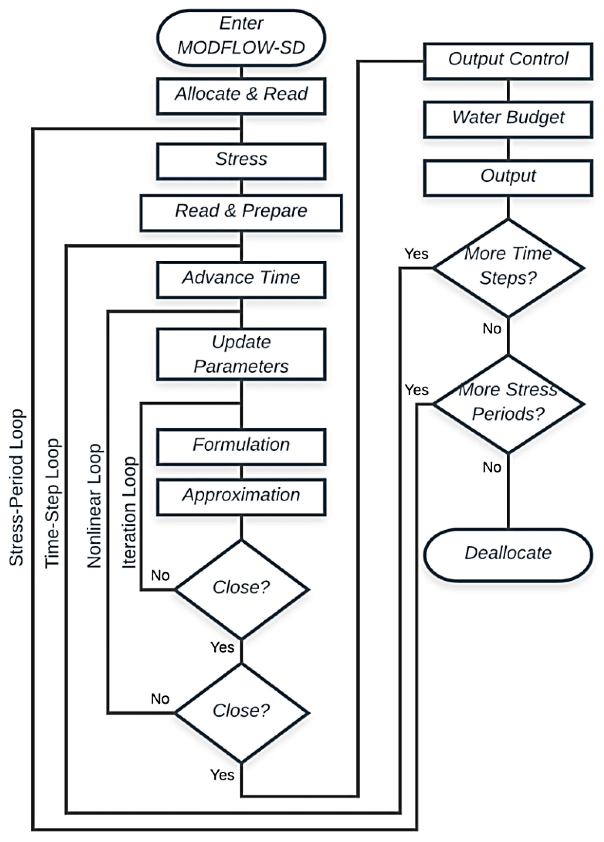
2.4. Stress-Dependent Groundwater Flow Model

MODFLOW employs a finite difference method to approximate Equation (1) and calculate groundwater heads and flows. To model hydraulic head distribution in a formation, including confined and unconfined aquifers with linear and nonlinear boundary conditions, MODFLOW utilizes linear and nonlinear numerical solution methods [13].

The stress-dependent groundwater model, MODFLOW-SD, is a modified version of MODFLOW to approximate the nonlinear groundwater flow Equation (2). The finite difference form of Equation (2) is a modified form of MODFLOW finite-difference formulation with stress-dependent coefficients, written as follows:

$$\begin{array}{c}\begin{array}{ll}C{C}_{i-\frac{1}{2},j,k}^{m,n-1}{h}_{i-\frac{1}{2},j,k}^{m,n}& +C{R}_{i,j-\frac{1}{2},k}^{m,n-1}{h}_{i,j-\frac{1}{2},k}^{m,n}+C{V}_{i,j,k-\frac{1}{2}}^{m,n-1}{h}_{i,j,k-\frac{1}{2}}^{m,n}\\ & +(-C{C}_{i-\frac{1}{2},j,k}^{m,n-1}-C{R}_{i,j-\frac{1}{2},k}^{m,n-1}-C{V}_{i,j,k-\frac{1}{2}}^{m,n-1}-C{C}_{i+\frac{1}{2},j,k}^{m,n-1}-C{R}_{i,j+\frac{1}{2},k}^{m,n-1}-C{V}_{i,j,k+\frac{1}{2}}^{m,n-1}+HCO{F}_{i,j,k}^{m,n})\\ & h_{i,j,k}^{m,n}+C{C}_{i+\frac{1}{2},j,k}^{m,n-1}{h}_{i+\frac{1}{2},j,k}^{m,n}+C{R}_{i,j+\frac{1}{2},k}^{m,n-1}{h}_{i,j+\frac{1}{2},k}^{m,n}+C{V}_{i,j,k+\frac{1}{2}}^{m,n-1}{h}_{i,j,k+\frac{1}{2}}^{m,n}=RH{S}_{i,j,k}^{m,n}\end{array}\\ RH{S}^{m,n}=-{\displaystyle {\displaystyle \sum }_{k=1}^{n2}}{Q}_{s,k}-{\displaystyle {\displaystyle \sum }_{k=1}^{n1}}{C}_{b,k}^{m,n-1}{h}_{b,k}-\frac{S_c^{m,n-1}{h}^{m-1}}{t^m-t^{m-1}}\\ HCO{F}^{m,n}=-{\displaystyle {\displaystyle \sum }_{k=1}^{n1}}{C}_{b,k}^{m,n-1}-\frac{S_c^{m,n-1}}{t^m-t^{m-1}}\end{array}$$

where the subscripts i, j, and k denote the cell column, row, and layer; m is the time step for which the heads are calculated; n is the number (or the level) of the iteration in iteration loop; $S_c$ is the storage coefficient; $Q_s$ is the head independent specific boundary flow; and $h_b$ are the flow conductance and boundary head, respectively; n1 and n2 are the numbers of head-dependent and specific flow boundaries; and CC, CR, and CV are conductance coefficients along column, row, and vertical directions, respectively. In MODFLOW, these conductance coefficients are assumed to be constant for confined layers and variable for unconfined one. In contrast, in the stress-dependent model, the head-dependent coefficients of CC, CR, CV, and $S_c$ are required to be updated in each iteration using head at the end of pervious iteration. RHS and HCOF in this equation are coefficients related to storage and sinks/sources terms.

The entire system of equations of the form of Equation (16) can be written in the matrix form to be solved using the linear solver already available to use with MODFLOW. Two packages, NONK for head-dependent hydraulic conductivity, and NONS, for head-dependent specific storage, have been developed to update head-dependent coefficients of Equation (16) based on exponential stress-stress behavior. Major input arrays for NONK and NONS packages are Initial horizontal and vertical hydraulic conductivities; initial specific storage; depth, total geostatic stress; compression index; recompression index; and hydraulic conductivity change index.

To deal with the material nonlinearity, a nonlinear loop was added to the main code of MODFLOW. Hence, the modified program includes four following nested loops: stress-period loop, time-step loop, nonlinear loop, and iteration loop. Head-dependent parameters, including hydraulic conductivity and specific storage, are updated within the nonlinear loop and via the update parameters process until the predefined convergence criterion is met. The flowchart of MODFLOW-SD is shown in Figure 2.

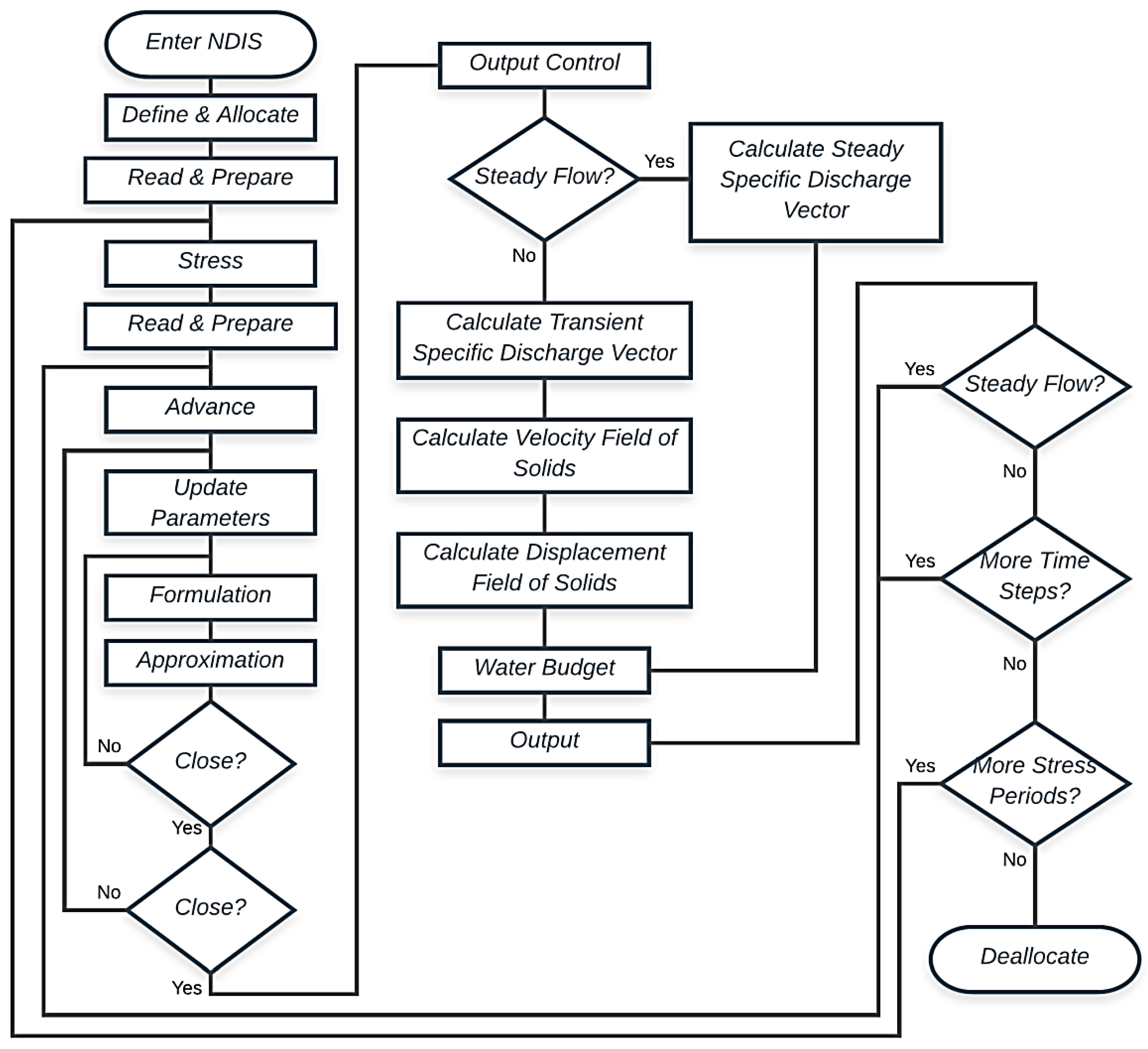
2.5. Stress-Dependent Land Movement Model

NDIS is a further developed version from DIS that assumes constant K and Ss [19] and a self-coded new module to simulate land movements by using a stress-dependent groundwater flow model. Compared to other land subsidence models in which the displacement field is calculated by integrating strain over space, these packages integrate the skeletal flux terms over time to approximate displacement.

The NDIS module was incorporated into the parent code MODFLOW-SD equipped with NONK and NONS packages to be able to simulate transient movement of an aquifer system with sedimentary materials with nonlinear stress-strain behavior. Figure 3 shows the NDIS package flowchart. For each stress period, firstly, the specific discharge vector for steady state condition is computed. Then, for each time step of that stress period, the specific discharge vector for transient condition is calculated. The difference of these two is used to estimate the velocity field of solids (Equation (5)). The velocity field of solids and the length of each time step are used to compute the displacement field of the skeletal frame across every cell wall.

NDIS, similar to other MODFLOW land subsidence packages, e.g., IBS1 and SUB-WT, does not consider the delayed dissipation of unequilibrated heads. It assumes that a head change applying to the volume of fine-grained compressible materials results in drainage of water without any time delays. Hence, the results of NDIS for vertical land movements are analogous to the land subsidence calculated by the SUB package using the no-delay option.

3. Numerical Modeling Results and Discussion

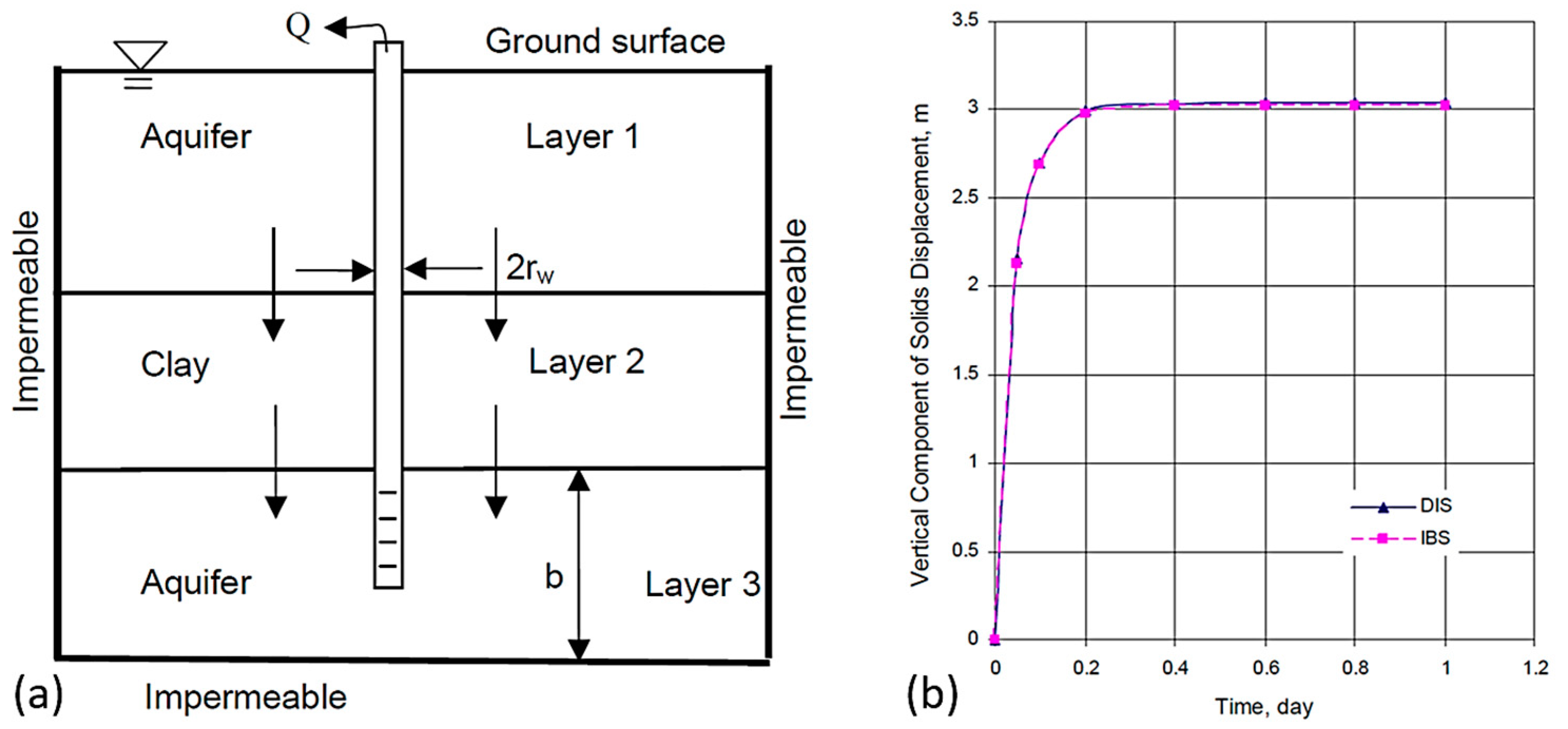
3.1. Validation of Land Subsidence Model with Constant Parameters

The DIS results (identical to NDIS with constant parameters) for vertical subsidence were checked against the IBS1 package, which is identical to SUB package with no-delay option. Zhang (2009) validated the DIS results for the aquifer system shown in Figure 4a. To compare the two models appropriately, the constant head boundary condition for the top layer and the no flow boundary conditions for the rest of the layers within a single column were selected. Pumping, at a constant rate of 10 ${\mathrm{m}}^3/\mathrm{d}\mathrm{a}\mathrm{y}$ for a one-day period, was performed [19]. Figure 4b shows the results for vertical land movements. The two models gave identical results showing validation of the DIS model or the NDIS model with constant parameters.

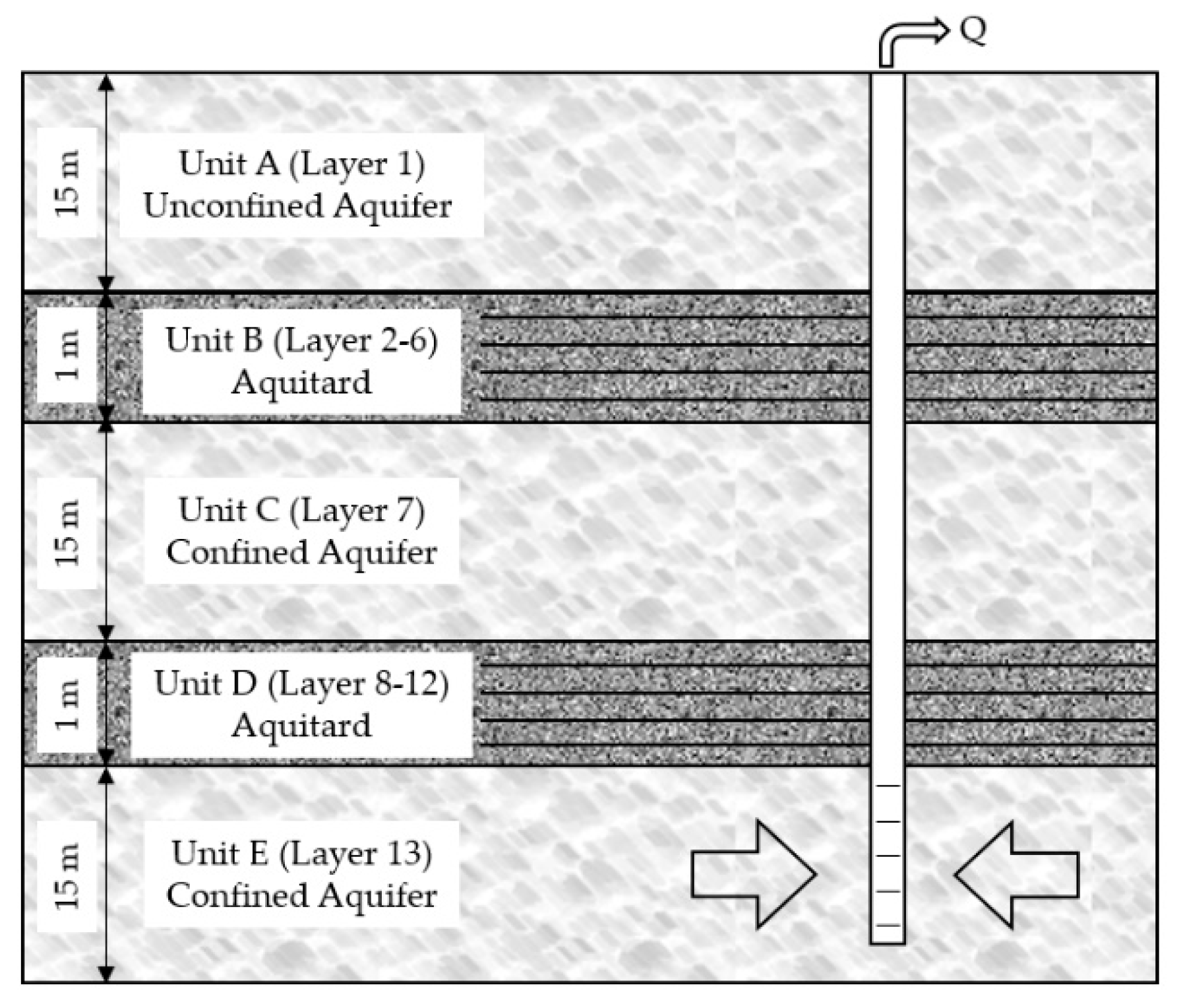
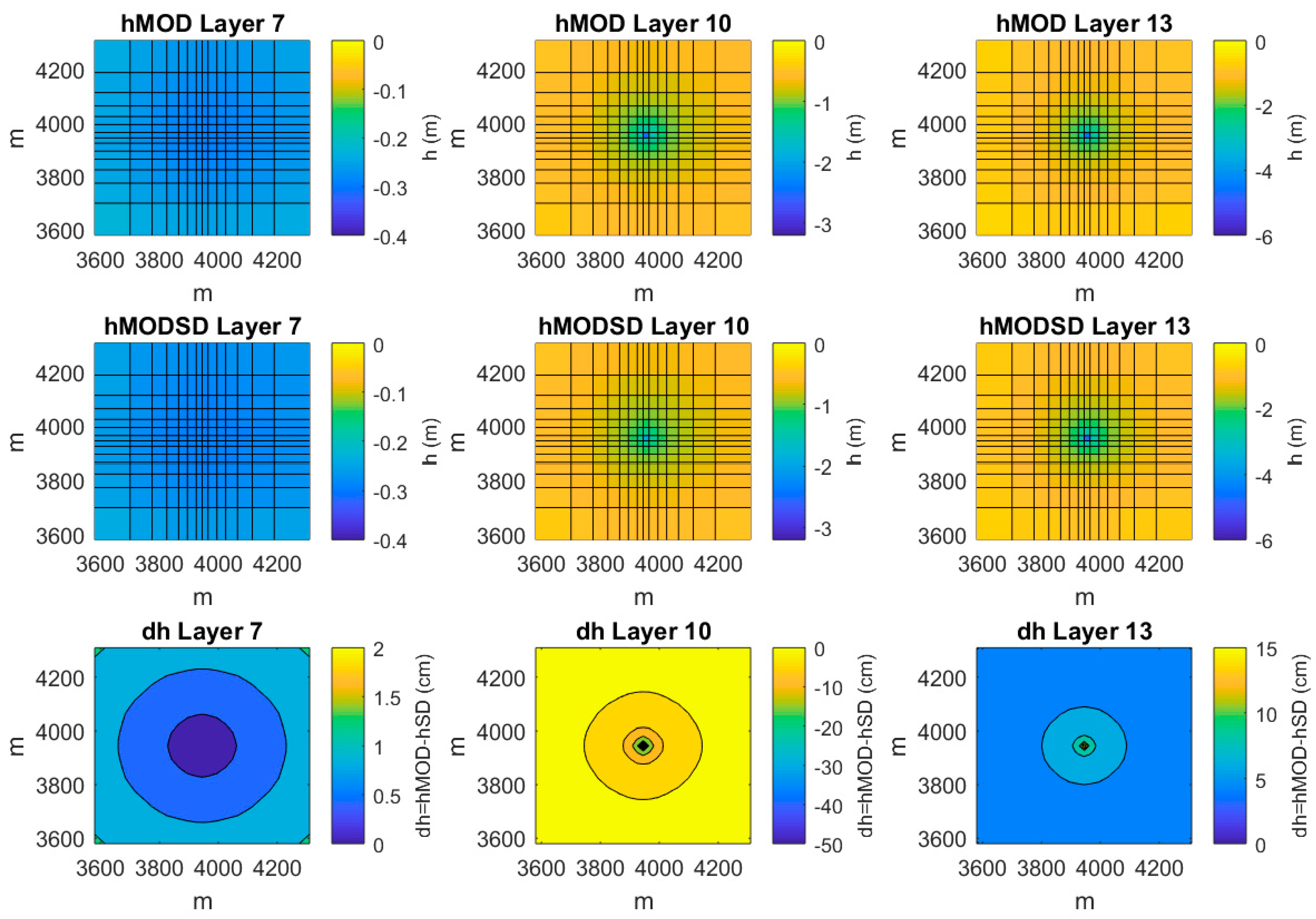
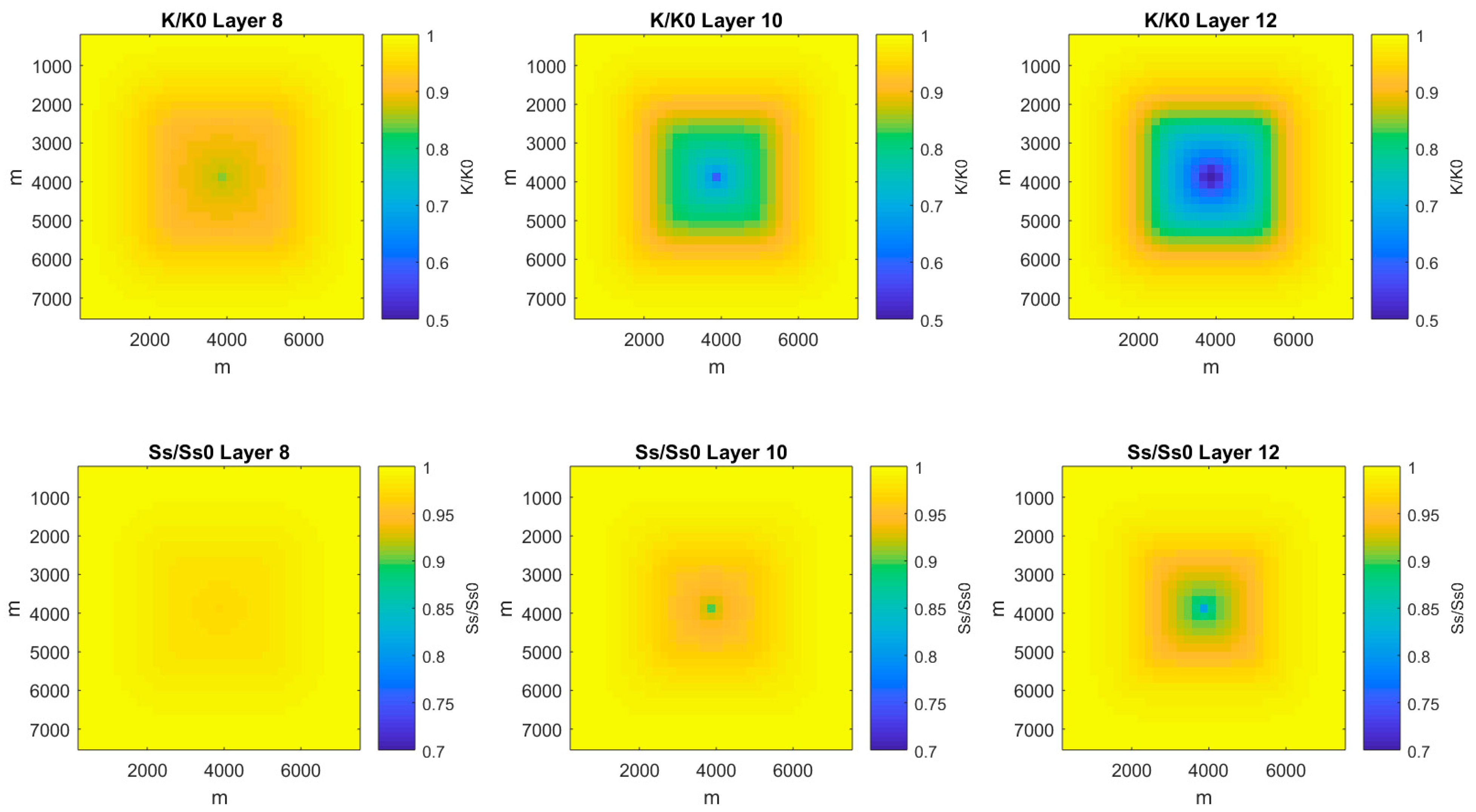
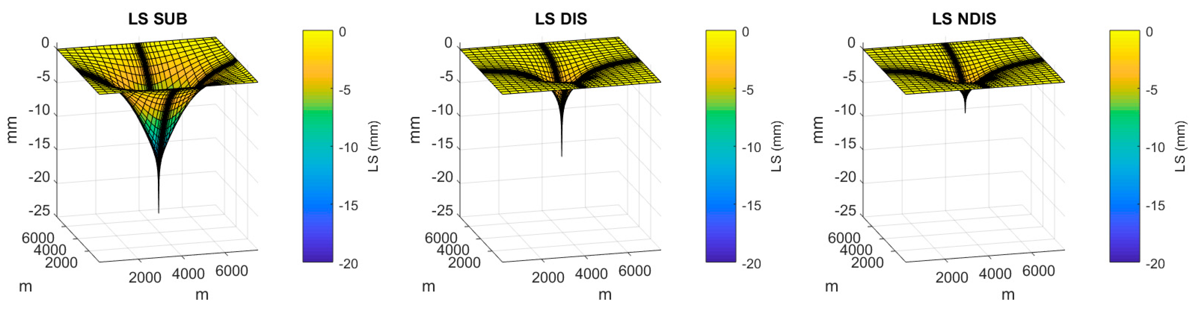
3.2. Sample Simulation

A conceptual model was considered for numerical modeling to evaluate the stress-dependent model. For the purpose of comparison, the results of hydraulic head calculated by MODFLOW and MODFLOW-SD, and the results of vertical land movement calculated by NDIS, DIS, and SUB packages (using a no-delay option) were compared.

The considered conceptual model, Figure 5, is a five-layer aquifer system comprising three aquifers and two aquitards as well as a pumping well fully penetrating into the third aquifer. In this model, the upper aquitard (unit B) is sandwiched with an overlying unconfined aquifer (unit A) and an underlying confined aquifer (unit C), and the lower aquitard (unit D) is sandwiched with two confined aquifers (unit C and unit E). The pumping well sits at the center of the grid and discharged from the second confined aquifer (unit E) with the constant rate of 3000 ${\mathrm{m}}^3/\mathrm{d}\mathrm{a}\mathrm{y}$ for 100 days. Non-uniform grids are employed for the horizontal space discretization of this model. This allows the grid to be more refined in regions where strong hydraulic head gradients are expected. Grid cells sizes are from 10 to 400 m and each layer is horizontally discretized by 37 rows and 37 columns. To trace the compaction of each layer accurately, the whole layer of each confining unit was divided into five slices. Hence, the discretized model consists of 13 layers in total. The hydrogeological and mechanical properties of the model are summarized in

Table 1. Hydrogeological and mechanical properties of the model.

Layer	Type	Material	Thickness (m)	${\mathit{K}}_{\mathit{x}0}{}^{*}$ (m/day)	${\mathit{K}}_{\mathit{z}0}{}^{*}$ (m/day)	${\mathit{S}}_{\mathit{s}\mathit{k}\mathit{v}0}{}^{**}$ (1/m)	${\mathit{S}}_{\mathit{s}\mathit{k}\mathit{e}0}{}^{**}$ (1/m)	${\mathit{S}}_{\mathit{y}}$	${\mathit{C}}_{\mathit{K}}$	${\mathit{C}}_{\mathit{c}}$	${\mathit{C}}_{\mathit{r}}$
1	unconfined aquifer (Unit A)	sand	15	50	5	${10}^{-4}$	${10}^{-4}$	0.2	0.5	0.05	0.05
2–6	Aquitard (Unit B)	clay	0.2	${10}^{-2}$	${10}^{-3}$	${10}^{-3}$	$5\times {10}^{-5}$	-	0.2	1.00	0.2
7	confined aquifer (Unit C)	sand	15	50	5	${10}^{-5}$	${10}^{-5}$	-	0.5	0.05	0.05
8–12	Aquitard (Unit D)	clay	0.2	${10}^{-2}$	${10}^{-3}$	${10}^{-3}$	$5\times {10}^{-5}$	-	0.2	1.00	0.2
13	confined aquifer (Unit E)	sand	15	50	5	${10}^{-5}$	${10}^{-5}$	-	0.5	0.05	0.05

* $K_{x0}$, $K_{z0}$: Initial hydraulic conductivity in horizontal and vertical directions. ** $S_{skv0}$, $S_{ske0}$: Initial inelastic and elastic specific storages.

. The lateral boundaries of the model were specified as constant-head boundaries and the initial hydraulic head, $h_0$, was assumed to be zero.

Two parameters of ${\sigma }_v$ and $z$ need to be predefined considering the geometry and material types of the model. Depth, $z$, is the elevation of middle point of each layer and the reference elevation is assumed to be on the earth surface. The unit weight of soil and the coefficient of earth pressure at rest, $k_o$, can be used to calculate the initial effective and total volume stresses for each layer. Empirical equations $k_o=1-sin\left(\phi \right)$ for sand [34] and $k_o=0.19+0.233log \left(PI\right)$ for clay [35], where $\phi$ is the friction angle and PI is the plasticity index, were used to calculate the coefficient of earth pressure at rest. Effective volume stress then were calculated using ${\sigma }_v^{\prime }={\sigma }_z^{\prime }\left(1+2k_o\right)/3$, where ${\sigma }_z^{\prime }$ is the effective vertical stress. Geostatic properties of the model are listed in

Table 2. Geostatic properties of the model.

Layer	Z* (m)	${\mathit{\sigma }}_{\mathit{v}}^{\prime }$ (KPa)
1	−7.5	93
2	−15.1	225
3	−15.3	228
4	−15.5	231
5	−15.7	234
6	−15.9	236
7	−23.5	290
8	−31.1	463
9	−31.3	466
10	−31.5	469
11	−31.7	471
12	−31.9	474
13	−39.5	488

.

Results of hydraulic heads calculated by MODFLOW and MODFLOW-SD for layer 7 (the first confined aquifer, unit C), layer 10 (the middle layer in second confining unit, unit D), and layer 13 (the second confined aquifer, unit E) are shown in Figure 6. As the difference between the two models shows, MODFLOW slightly overestimates heads in aquifer units with a higher permeability and lower compressibility, units C and D in this case. For the confining unit, layer 10, the overestimation is about 20%. In some subsidence models, e.g., IBS1 model and SUB model, compaction is assumed to be linearly proportional to change in hydraulic head. Hence, any error in head calculated by the groundwater model would affect the predicted compaction.

Changes in hydraulic conductivity for different locations within the aquifer system are shown in Figure 7. Figure 8 shows the change in hydraulic conductivity and specific storage at the top (layer 8), middle (layer 10), and bottom (layer 12) of the second confining unit, unit D. This figure shows how the parameters of the compressible confining units would change under a nonlinear stress-strain relation. As it could be predicted, the lowest layer of the confining unit adjacent to the pumped aquifer would be impacted the most. Moreover, a homogeneous highly compressible formation, unit D in this case, is transformed to a horizontally and vertically heterogenous one. This transformation changes the groundwater flow pattern and subsequently the predicted subsidence.

For the considered groundwater extraction scenario, land subsidence that occurred on the surface was modeled using the SUB, DIS, and NDIS models. The SUB and DIS models use hydraulic heads calculated by MODFLOW and NDIS uses MDFLOW-SD results to calculate layers compaction. Models were set to include all layers in the aquifers and aquitards units contributing, but to different degrees, to accumulated subsidence on the surface.

Figure 9 shows the predicted subsidence calculated by the three models for the considered conceptual model. The differences between subsidence calculated by the three models are shown in Figure 10. Figure 11 shows these differences at the profile passing through the center of the grid. Results show that the maximum subsidence occurs at the vicinity of the pumping well with the magnitude of 25 mm, 17 mm, and 11 mm for the SUB, DIS, and NDIS models, respectively. The SUB model predicts a significantly larger sinking and a wider area of compaction around the pump. This is because, firstly, the volume strain for SUB model is entirely converted to vertical strain and, secondly, the assumption of linear strain with constant compressibility is employed in the SUB model. In contrast, the DIS and NDIS models use vertical specific discharges to calculate vertical deformation. The assumption of horizontally constrained strain employed in the SUB model was not used in the DIS and NDIS models. Compared to DIS model, NDIS showed a smaller subsidence with limited area of compaction around the pump. For this stress-dependent model, change in soil parameters was significant for highly compressible confining units and near the pumping well that declines layers compaction due to soil-hardening.

For a site-specific case, parameters $C_c,C_r,C_k,K_{x0},K_{z0},S_{skv0},\mathrm{and}{S}_{ske0}$ for NDIS in Table 1 would be better calibrated with field aquifer system compaction data with UCODE (the Computer Code for Universal Inverse Modeling) [36] or PEST (the Model-Independent Parameter Optimiser) [37], based on a developed groundwater flow model coupled with NDIS. Initial values for $K_{x0},K_{z0},S_{skv0},\mathrm{and}{S}_{ske0}$ can be obtained from graphic-analysis of groundwater level fluctuations and compaction [38,39] and aquifer testing results. Initial values for $C_c,C_r,\mathrm{and}{C}_k$ can be obtained from consolidation tests ($e-\log \left({\sigma }_v^{\prime }\right)$ curve and $e-\log \left(K\right)$ curve) other than such values in Table 1.

4. Conclusions

The stress-dependent groundwater flow model, MODFLOW-SD, has been developed and coupled with the nonlinear subsidence model, NDIS, to predict groundwater extraction-related subsidence. MODFLOW-SD is a modified version of MODFLOW and includes two new packages, NONK and NONS, to update hydraulic conductivity and skeletal storage due to change in effective stress. The NDIS model is a nonlinear form of the DIS model to predict land subsidence using the specific discharge vector. This new model does not adopt the two simplifications used in other coupled models, (e.g., the SUB package of MODFLOW), namely: (1) Ignoring stress-dependency of hydraulic conductivity and skeletal storage and (2) ignoring the horizonal strain and converting the entire volume strain to vertical strain.

For the considered conceptual model, comparison of the results showed that hydraulic head calculated by MODFLOW was slightly underestimated for aquifer units and significantly overestimated for confining ones. That would subsequently result in overestimation of vertical subsidence occurred on the surface. Simulation results showed that applied stress due to pumping changed initially homogeneous layers to heterogeneous ones. The magnitude of such changes significantly depends on the ratio of $C$ (compression or recompression index) and $C_k$ (hydraulic conductivity change index).

Both DIS and NDIS models use the vertical component of the three-dimensional displacement vector to calculate vertical deformation. Compared to subsidence calculated by NDIS, the SUB model predicted a significantly larger deformation. This is because, firstly, the volume strain is entirely converted to vertical strain and, secondly, the aquifer parameters are not stress-dependent.

Although all three models match an observed subsidence data, the NDIS model proposes smaller aquifer parameters, including hydraulic conductivity and skeletal storage. Therefore, larger parameters proposed by DIS and SUB models will overestimate future subsidence. Furthermore, NDIS is more likely to provide a more accurate compaction model for a complex aquifer system with vertically variable compaction indices, such as lacustrine materials deposited at the volcanic valley of Mexico City.

References

1. Ireland, R.L.; Poland, J.F.; Riley, F.S. Land Subsidence in the San Joaquin Valley, California, as of 1980; US Geological Survey: Reston, VA, USA, 1984. [Google Scholar]
2. Galloway, D.L.; Burbey, T.J. Review: Regional land subsidence accompanying groundwater extraction. Hydrogeol. J. 2011, 19, 1459–1486. [Google Scholar] [CrossRef]
3. Link, L.E. The anatomy of a disaster, an overview of Hurricane Katrina and New Orleans. Ocean Eng. 2010, 37, 4–12. [Google Scholar] [CrossRef]
4. Coplin, L.S.; Galloway, D.L. Houston-Galveston, Texas: Managing coastal subsidence. In Land Subsidence in the United States; US Geological Survey: Reston, VA, USA, 1999; pp. 35–46. [Google Scholar]
5. Liu, Y.; Li, J.; Fang, Z.N.; Liu, Y.; Li, J.; Fang, Z.N. Groundwater Level Change Management on Control of Land Subsidence Supported by Borehole Extensometer Compaction Measurements in the Houston-Galveston Region, Texas. Geosciences 2019, 9, 223. [Google Scholar] [CrossRef]
6. Chaussard, F.; Amelung, E.; Abidin, H.; Hong, S.-H. Sinking cities in Indonesia: ALOS PALSAR detects rapid subsidence due to groundwater and gas extraction. Remote Sens. Environ. 2013, 128, 150–161. [Google Scholar] [CrossRef]
7. Ng, A.H.-M.; Ge, L.; Li, X.; Zhang, K. Monitoring ground deformation in Beijing, China with persistent scatterer SAR interferometry. J. Geod. 2012, 86, 375–392. [Google Scholar] [CrossRef]
8. Gabrysch, R.K. Ground-Water Withdrawals and Land-Surface Subsidence in the Houston-Galveston Region, Texas, 1906–1980; US Geological Survey: Reston, VA, USA, 1982. [Google Scholar]
9. Poland, J.F.; Ireland, R.L. Land Subsidence in the Santa Clara Valley, California, as of 1982; US Geological Survey: Reston, VA, USA, 1988.
10. Yan, Y.; Doin, M.P.; Lopez-Quiroz, P.; Tupin, F.; Fruneau, B.; Pinel, V.; Trouvé, E. Mexico City Subsidence Measured by InSAR Time Series: Joint Analysis Using PS and SBAS Approaches. IEEE J. Sel. Top. Appl. Earth Obs. Remote Sens. 2012, 5, 1312–1326. [Google Scholar] [CrossRef] [Green Version]
11. Mahmoudpour, M.; Khamehchiyan, M.; Nikudel, M.R.; Ghassemi, M.R. Numerical simulation and prediction of regional land subsidence caused by groundwater exploitation in the southwest plain of Tehran, Iran. Eng. Geol. 2016, 201, 6–28. [Google Scholar] [CrossRef]
12. Meade, R.H. Removal of Water and Rearrangement of Particles During the Compaction of Clayey Sediments—Review; US Government Printing Office: Washington, DC, USA, 1964.
13. McDonald, M.G.; Harbaugh, A.W. A Modular Three-Dimensional Finite-Difference Ground-Water Flow Model; US Geological Survey: Reston, VA, USA, 1988.
14. Leake, S.A.; Prudic, D.E. Documentation of a Computer Program to Simulate Aquifer-System Compaction Using the Modular Finite-Difference Ground-Water Flow Model; US Department of the Interior: Washington, DC, USA; US Geological Survey: Reston, VA, USA, 1991.
15. Hoffmann, J.; Leake, S.A.; Galloway, D.L.; Wilson, A. MODFLOW-2000 Ground-Water Model—User Guide to the Subsidence and Aquifer-System Compaction (SUB) Package. No 03-233; Geological Survey: Washington, DC, USA, 2003; p. 46.
16. Leake, S.A.; Galloway, D.L. MODFLOW Ground-Water Model—User Guide to the Subsidence and Aquifer-System Compaction Package (SUB-WT) for Water-Table Aquifers; US Geological Survey: Reston, VA, USA, 2007; p. 42.
17. Burbey, T.J. A Finite-Difference Model of Three-Dimensional Granular Displacement. Ph.D. Thesis, University of Nevada, Reno, NV, USA, 1994. [Google Scholar]
18. Burbey, T.J. Storage coefficient revisited—Is purely vertical strain a good approximation? Ground Water 2001, 39, 458–464. [Google Scholar] [CrossRef] [PubMed]
19. Zhang, L. A Model for Transient Three-Dimensional Underground Deformation in Response to Groundwater Pumpage. Ph.D. Thesis, Morgan State University, Baltimore, MD, USA, 2009. [Google Scholar]
20. Kang, D.H.; Lee, H.J.; Li, J. Modeling of land movement due to groundwater pumping from an aquifer system with stress-dependent storage. In Proceedings of the Shale Energy Engineering 2014: Technical Challenges, Environmental Issues, and Public Policy, Pittsburgh, PA, USA, 21–23 July 2014; pp. 1–10. [Google Scholar]
21. Lee, H.J.; Li, J. Numerical modeling of aquifer radial movement caused by groundwater pumping. In Proceedings of the World Environmental and Water Resources Congress 2015: Floods, Droughts, and Ecosystems, Austin, TX, USA, 17–21 May 2015; pp. 595–605. [Google Scholar]
22. Rashvand, M.; Li, J. Simulation of an aquifer system changing from homogeneous to heterogeneous one due to head-dependent conductivity. In Proceedings of the International Perspective on Water Resources and the Environment., Wuhan, China, 4–6 January 2017. [Google Scholar]
23. Owolabi, O.; Rashvand, M.; Liu, Y.; Li, J. Laboratory investigation of stress-dependency and anisotropy of hydraulic conductivity. In Proceedings of the International Perspective on Water Resources and the Environment, Wuhan, China, 4–6 January 2017. [Google Scholar]
24. Li, J.; Ding, D. Modeling 3D land subsidence due to groundwater pumping with a variable parameter. In Global View of Engineering Geology and the Environment; CRC Press: Boca Raton, FL, USA, 2013; pp. 457–462. [Google Scholar]
25. Helm, D.C. Horizontal aquifer movement in a Theis-Thiem confined system. Water Resour. Res. 1994, 30, 953–964. [Google Scholar] [CrossRef]
26. Gersevanov, N. The Foundation of Dynamics of Soils; Stroiizdat: Leningrad (Saint Petersburg), Russia, 1934. (In Russian) [Google Scholar]
27. Helm, D.C. Latrobe Valley Subsidence Predictions, The Modeling of Time-Dependent Ground Movement Due to Groundwater Withdrawal; State Electricity Commission of Victoria: Melbourne, Australia, 1984. [Google Scholar]
28. Helm, D.C. Hydraulic forces that play a role in generating fissures at depth. Bull. Assoc. Eng. Geol. 1994, 31, 293–304. [Google Scholar] [CrossRef]
29. Das, B.M. Principles of Geotechnical Engineering, 3rd ed.; PWS Publishing Co.: Boston, MA, USA, 1994. [Google Scholar]
30. Taylor, D.W. Fundamentals of Soil Mechanics; John Wiley and Sons Inc.: Hoboken, NJ, USA, 1948. [Google Scholar]
31. Terzaghi, K. Settlement and consolidation of clay. Eng. News Rec. 1923, 95, 874–878. [Google Scholar]
32. Hubbert, M.K. The theory of ground-water motion. J. Geol. 1940, 48, 785–944. [Google Scholar] [CrossRef]
33. Harbaugh, A.W. MODFLOW-2005: The U.S. Geological Survey Modular Ground-Water Model: The Ground-Water Flow Process; US Geological Survey: Reston, VA, USA, 2005.
34. Jaky, J. Pressure in soils. In Proceedings of the 2nd International Conference on Soil Mechanics and Foundation Engineering, Rotterdam, The Netherlands, 21–30 June 1948; pp. 103–107. [Google Scholar]
35. Alpan, I. The empirical evaluation of the coefficient K0 and K0R. Soils Found. 1967, 7, 31–40. [Google Scholar] [CrossRef]
36. Poeter, E.P.; Hill, M.C. Documentation of UCODE, a Computer Code for Universal Inverse Modeling; Diane Publishing: Collingdale, PA, USA, 1998. [Google Scholar]
37. Doherty, J. PEST, Model-Independent Parameter Estimation—User Manual, 5th ed.; Watermark Computing: Brisbane, Australia, 2004. [Google Scholar]
38. Riley, F.S. Analysis of borehole extenso meter data from central California. Int. Assoc. Sci. Hydrol. Publ. 1969, 89, 423–431. [Google Scholar]
39. Liu, Y.; Helm, D.C. Inverse procedure for calibrating parameters that control land subsidence caused by subsurface fluid withdrawal: 1. Methods. Water Resour. Res. 2008, 44, 1–16. [Google Scholar] [CrossRef]
Figure 1. Relations of dimensionless R S s = S s / S s 0 (a), R k = K / K 0 (b), and R D = D / D 0 (c) against normalized effective stress R S = σ v / σ v 0 with four different values of R C = C / C k (=0, 0.1, 1, and 10).
Hydrology 06 00078 g001
Figure 2. MODFLOW-SD (modified USGS Modular Three-Dimensional Groundwater Flow Model) flowchart to simulate stress-dependent ground-water flow (modified from [33]).
Hydrology 06 00078 g002
Figure 3. NDIS Flowchart to simulate movement of an aquifer system with sedimentary material having nonlinear stress-strain behavior.
Hydrology 06 00078 g003
Figure 4. (a) Conceptual model to evaluate subsidence calculated by DIS package (identical to NDIS with constant parameters) and IBS (Interbed Storage) package. (b) Comparison of vertical deformation calculated by the two models [19].
Hydrology 06 00078 g004
Figure 5. Conceptual model including a five-layer aquifer system comprising three aquifers and two aquitards, as well as a pumping well fully penetrating the third aquifer.
Hydrology 06 00078 g005
Figure 6. Results of groundwater heads calculated by MODFLOW and MODFLOW-SD for layer 7 (the first confined aquifer, unit C), layer 10 (the middle layer in second confining unit, unit D), and layer 13 (the second confined aquifer, unit E). dh is the difference between heads estimated by the two models.
Hydrology 06 00078 g006
Figure 7. Change in hydraulic conductivity for different locations within the aquifer system.
Hydrology 06 00078 g007
Figure 8. Change in hydraulic conductivity and specific storage at the top (layer 8), middle (layer 10), and bottom (layer 12) of the second confining layer, unit D. A homogeneous highly compressible formation, unit D in this case, is transformed to a horizontally and vertically heterogenous one.
Hydrology 06 00078 g008
Figure 9. Subsidence calculated by SUB, DIS, and NIDS packages for the conceptual model.
Hydrology 06 00078 g009
Figure 10. Differences between subsidence calculated by the three models. LS SUB-LS DIS: difference between subsidence calculated by SUB model and DIS model. LS DIS-LS NDIS: Difference between subsidence calculated by DIS model and NDIS model. LS SUB-LS NDIS: Difference between subsidence calculated by SUB model and NDIS model.
Hydrology 06 00078 g010
Figure 11. Differences between subsidence calculated by the three models at the profile passing through the center of the grid.
Hydrology 06 00078 g011