Real-Time Measurement of Flash-Flood in a Wadi Area by LSPIV and STIV

Abstract

Flash floods in wadi systems discharge large volumes of water to either the sea or the desert areas after high-intensity rainfall events. Recently, wadi flash floods have frequently occurred in arid regions and caused damage to roads, houses, and properties. Therefore, monitoring and quantifying these events by accurately measuring wadi discharge has become important for the installation of mitigation structures and early warning systems. In this study, image-based methods were used to measure surface flow velocities during a wadi flash flood in 2018 to test the usefulness of large-scale particle image velocimetry (LSPIV) and space–time image velocimetry (STIV) techniques for the estimation of wadi discharge. The results, which indicated the positive performance of the image-based methods, strengthened our hypothesis that the application of LSPIV and STIV techniques is appropriate for the analysis of wadi flash flood velocities. STIV is suitable for unidirectional flow velocity and LSPIV is reliable and stable for two-dimensional measurement along the wadi channel, the direction of flow pattern which varies with time.

1. Introduction

“Wadi” is an Arabic term commonly used to refer to an ephemeral river or valley in an arid region, such as in Middle Eastern countries. Monitoring the discharge of wadi flash floods is a major concern for the management of water resources and the reduction of disaster risk. Recently, extreme and frequent flooding has occurred in arid regions, resulting in significant economic and property losses. For instance, Oman was hit by a cyclone in July 2007 that killed 50 people, and the damage to properties was evaluated at 3.9 billion U.S. dollars [1]. According to flood discharge data recorded in Oman, significant flash floods have caused massive destruction of infrastructure and loss of human life [2]. In arid regions, flash flood warning systems are still limited and not effective due to the limitation of discharge monitoring and observational networks. However, flash floods have received more attention in the last decade due to climate change factors.

In October 2018, flash flood events increased in association with the frequency of extreme rainfall events and caused extensive destruction in most Middle Eastern arid areas, for instance, in Petra, Jordan, and in Kuwait, Qatar, Saudi Arabia, and Oman. These areas suffer from a lack of expertise resulting in improper planning and management. However, because the monitoring of rainfall, water level, and discharge rates in these areas is lacking, it is difficult to calibrate and validate the hydrological models used for wadi flash flood studies. Even though several hydrological models have been developed to simulate the rainfall–runoff process in river systems, the flow characteristics of wadi systems in arid regions are complicated and involve various parameters, for example, steep topography and no baseflow, therefore, there are insufficient measurement data [3]. This has resulted in the poor design and selection of mitigation structures, such as culverts, embankments, drainage systems, and dams.

After cyclone Gonu hit Oman in 2007, the local government upgraded all monitoring systems, and now, most strategic wadi systems are equipped with rainfall and water level stations. The main challenge with the installed ground-based stations in most wadis in Oman is the ad hoc design and selection of the sensor network. Wider challenges to the establishment of a novel observational network ad hoc-designed measurement system are summarized in reference [4]. However, flow discharge measurements are not available for some of these wadis. To our knowledge, no specific monitoring device has been developed for ephemeral rivers such as those in the wadi system. Consequently, an ad hoc sensors and observation approach can provide accurate and high-quality measurements for specific hydrological issues with low-cost and modified sensors [4]. The flow velocities in wadi systems are measured by using flow meters during flash flood recessions and base flows, this provides poor-quality data. Although various other techniques are available to measure water velocities in river systems, such as acoustic doppler velocimeters and acoustic doppler current profilers. By using surface velocity radar (SVR), Matilde et al. [5] examined different flows and reported a maximum velocity in wadi flash floods of between 0.79 and 2.58 m/s. However, because of the high volume of floating debris and difficulties determining the beginning of flash floods, all of these methods are unsuitable for monitoring flash floods in wadi systems.

Conventional methods may be used to monitor flash floods in wadi systems, for instance, the measuring of water levels and the slope–area method to generate water level–discharge relationships (rating curves). However, the field measurements and observations for peak discharge values have a limited range for establishing accurate rating curves [6]. Moreover, the slope–area method in wadi systems relies on flood marks from post-flood surveys, for example, floating debris and sediments deposited on both banks of the channel, to obtain the water surface slope in each cross-sectional area, which affects the reliability of discharge predictions. The field measurements of water levels and cross-sectional surveys have uncertainties and sources of errors in the discharge measurements due to changing of the channel bed [7]. The hydrographs of flash floods in arid regions demonstrate a local point with sharp peaks of short duration after high-intensity rainfall events.

The basics of conventional image-based techniques such as particle image velocimetry (PIV) have been reviewed in detail [8,9]. Image-based methods, such as large-scale particle image velocimetry (LSPIV) and space–time image velocimetry (STIV) techniques, are indirect methods used to convert images of free surface stream flow recorded on video to estimate flow velocity using image processing and analysis technologies [10]. Both techniques are visualization approaches that were developed from PIV in laboratory experiments [8,11]. The first field investigations of image velocimetry measurements were started in Japan in river environments [11,12].

There are many challenges to be considered when using LSPIV techniques, for instance, the lacking of surface wave and floating debris on the water surface, moreover, and availability of light reflection and vegetation increase the uncertainties of the final results. The percentage of error in estimated flow rate using LSPIV was within −5% to 7% [13]. A. A. Harpold et al. (2006) [14] tested the LSPIV method under different conditions and he found that on increasing the angle of camera to the channel bed, more error is generated in the image ortho-rectification. Additionally, the mean error of the LSPIV discharge measurements was less than 10% compared with wire discharge measurement for the same flow condition.

The utilization of natural tracers and water turbid current conditions can minimize the effects of sun reflection and enhance the estimated velocity results [15]. Various research studies have investigated the performance of various image-based methods in humid environments, such as LSPIV, Particle Tracking Velocimetry (PTV), and STIV [7,16].

The LSPIV technique is among the most commonly investigated type of flash flood monitoring systems, and several studies of image-based methods have been undertaken in riverine systems [5,6,7,8,9,10]. However, this is the first time that LSPIV and STIV have been implemented to measure the flow discharge of wadi floods in an arid environment. The main differences between wadi flash floods and normal river floods in humid environments are the occurrences and locality of the wadi flood with high flood peaks and rapid flow inundation. Thereby, using non-contact methods such as the LSPIV technique in a flash flood monitoring system will help to improve the quality of field measurements. This type of technique is dependent on measuring the surface flow velocity, which can then be utilized to compute the peak discharge. Previous publications have concluded that the LSPIV technique can be used to design real-time flood monitoring network systems, so this seems to be a reliable, innovative approach [17].

The STIV technique is dependent on surface textures, which include surface flow waves, brightness, and color variation, to measure surface flow velocity. This technique uses sequential frames over time changing with specified spacing in the search lines set parallel to the flow direction [15,16]. The main concept of this technique is extracting the brightness and texture information, which is called the image intensity distribution (IID), from sequentially recorded frames passing over the segment lines [17,18].

Remote image-based methods such as LSPIV and STIV have been widely applied to river channels to improve the accuracy of flow rate measurements. In addition, the visual investigations of surface flow features can assist the scientific understanding of the real situation and are a highly recommended method [19]. Finally, monitoring systems that use image analysis have an advantage of presenting clear visual images of real-time situations, which, by indicating the velocity of surface flow, can help prevent disasters. Therefore, LSPIV and STIV techniques used at remote monitoring stations are powerful and affordable hydrometric tools that can help measure surface flow velocity. The current paper aims to investigate the efficiency of using LSPIV and STIV techniques in wadi systems to obtain peak discharges for medium-sized flood events.

2. Materials and Methods

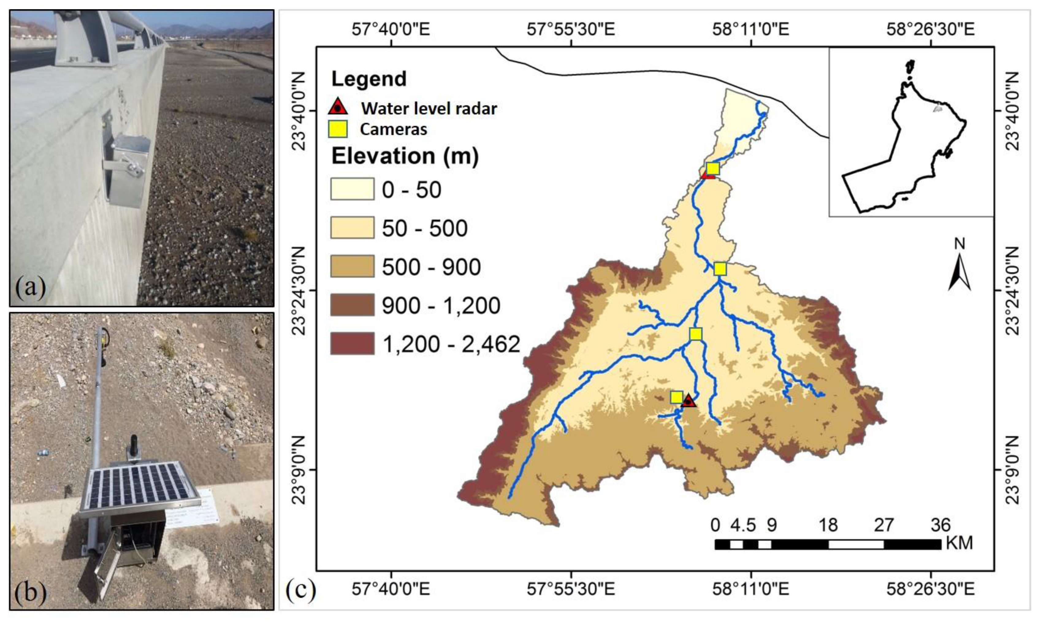
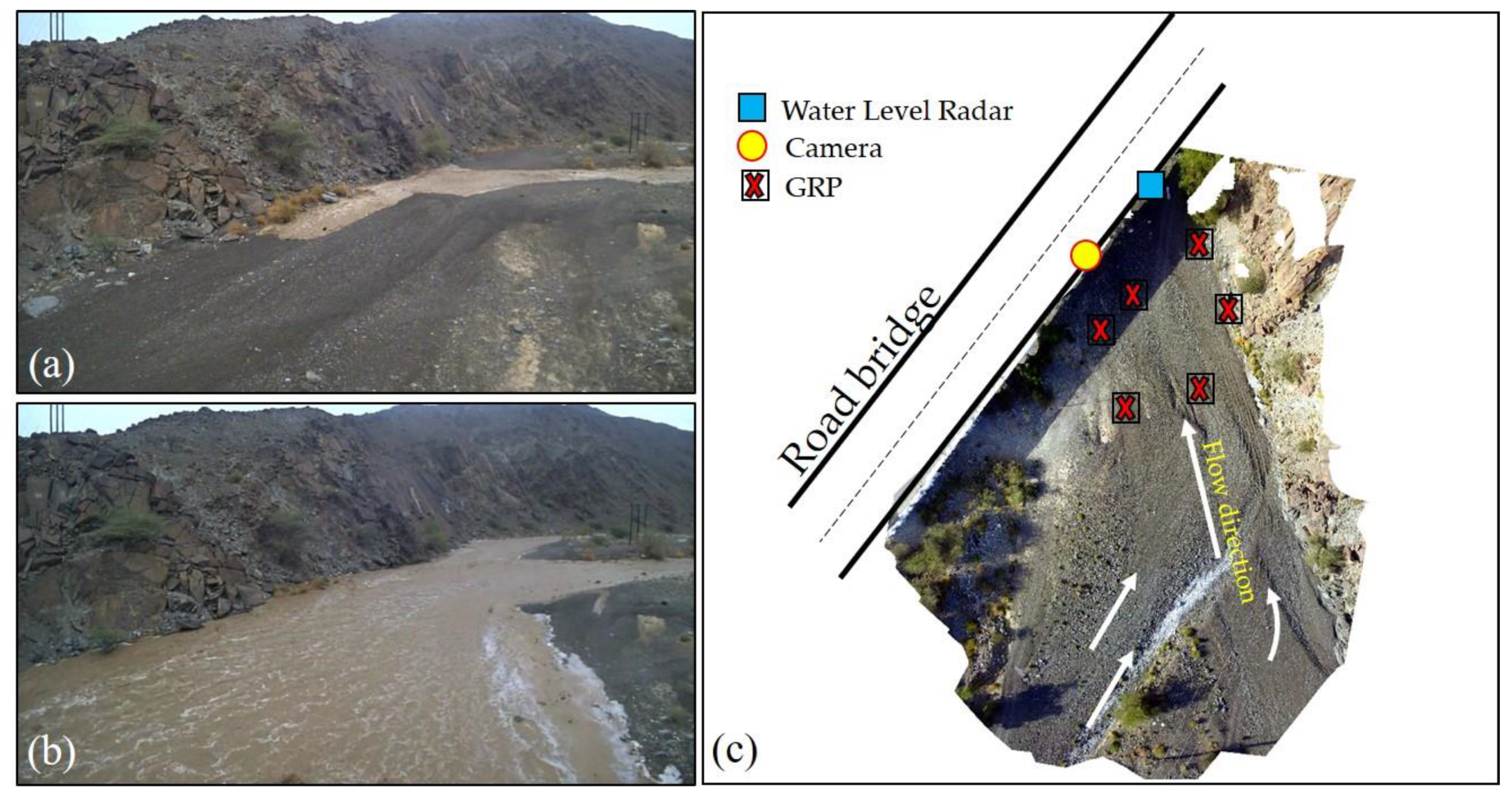
2.1. Study Area

The study area is located in the Wadi Samail catchment, northern Oman (Figure 1c), which has a drainage area of 1669 km² and two main types of channel bed: gravel and sand. The land cover is mainly bare rock with sparse vegetation, being located in a mountainous area, 76% slope of mountains [20]. The topography of the wadi channels is steep and narrow. To mitigate floods in this wadi, the government of Sultanate Oman constructed the Al khawd Dam as a mitigation structure. Moreover, rainfall and water level monitoring stations, operated by the Ministry of Regional

Municipalities and Water Resources, were installed along the wadi channels, and various elevated bridges were constructed where roads cross them. These elevated bridges were built in a very high elevation to free the Wadi channel from the crossing culvert. During the July 2007 flood in Oman significant failures and damages were observed in the embankments and culverts structures due to design mistakes and height of construction.

In 2016, we utilized these road bridges to install four cameras at four different locations along the wadi to capture images with a high angle of incidence to the upstream wadi and a number of conditional ground reference points (GRPs) for the analysis of large-scale flash flooding using LSPIV and STIV techniques. Consequently, on 28 October 2018, we captured a flood event with a peak discharge, estimated from a rating curve that relies on different slope area measurements, of 6.4 m³/s for the medium scale of flash flood. We then applied image-based methods to estimate the surface flow velocities of this event. This site was selected based on the availability of the water level gauging station and the slope area measurements for this area. Although, upstream of this catchment, it was always affected by local rainfall.

2.2. Camera Installation

Flash floods in wadi systems have been relatively infrequent and are unpredictable due to many factors such as the spatial and temporal variability of rainfall. A fixed camera was installed on a road bridge, housed in a steel box for protection, at a height of 7.9 m above the channel and set up to record video over the long interval since 2016 (Figure 1a). In this application, we used only one camera, located at the upstream reach of wadi Al-uqq (Figure 1b), to apply LSPIV and STIV techniques. A series of images were collected by the fixed camera during the event of 28 October at the rate of 30 frames per second, with an image resolution of 1280 × 720 pixels.

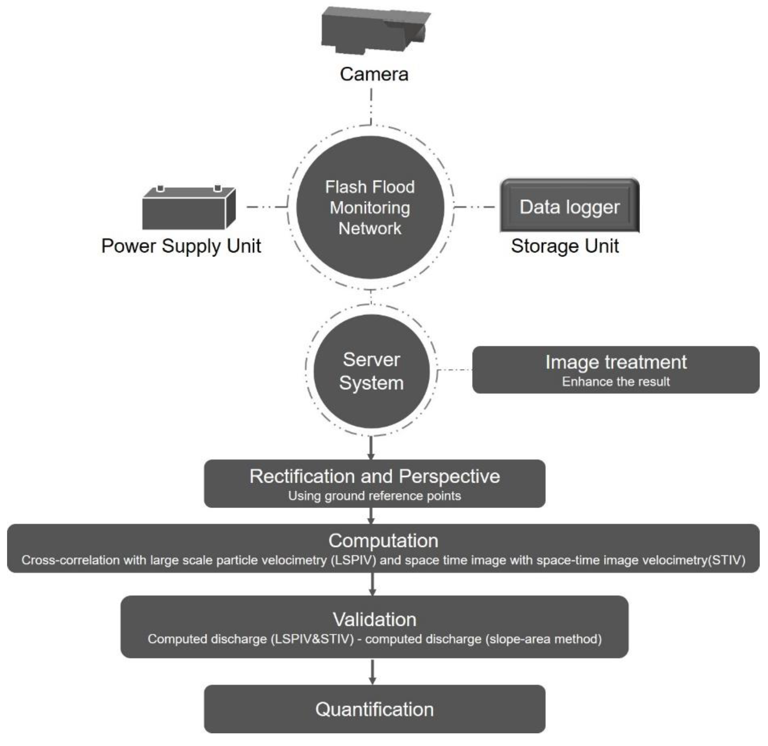
2.3. Image Processing

The flash flood surface flow images were recorded from a road bridge with an oblique angle. Therefore, all images were ortho-rectified and perspective-corrected to extract accurate surface flow data [11]. To apply this process, we used six GRPs, including x and y coordinates. The criteria for obtaining the GRPs involved photogrammetric processing, accomplished by collecting drone camera images of the channel bed morphology with high resolution. These images were converted to a digital elevation model (DEM) and spatial data. Subsequently, we selected a target reference point—natural features, such as stable rocks within the channel—to extract x and y coordinates from the DEM. Several studies in the literature suggest that structure-from-motion (SFM) software is a useful tool for processing images of complex structures and representing an accurate DEM [21,22]. The advantage of image processing is that it provides applicable spatial resolution for the extraction of relatively accurate DEMs [23]. Agisoft Photoscan Professional Edition (Agisoft LLC, St. Petersburg, Russia) was used to analyze images from a drone camera vertically mounted above the channel (Figure 2a). The surface flow velocity was analyzed by applying LSPIV with a cross-correlation algorithm [12] and STIV, using structural changes in the brightness of the water surface over time [17]. The flash flood in the wadi system had sufficient available floating debris, sediment clouds, free surface waves, and foams generated at the flow surface to use as natural seeding tracers, which can present precisely the local flow movements [11].

To produce a hydrograph with three points, we divided the analysis of the flash flood event into three sections: first, the rising limb, starting from zero flow; second, the peak flow; and third, the recession limb. The velocity and cross-sectional area obtained from the image-based processing were subsequently used to compute the discharge.

For the LSPIV technique, we used commercially available Dynamic Studio software (Dantec Dynamics A/S, Skovlunde, Denmark) to analyze the data with the essential correlation functions, filtering, and statistical calculations on the images to obtain the computed flow velocity and flow pattern. The directions and signs of surface flow and velocity vectors are derived based on the displacement of naturally occurring floating foams, color variation of the turbid water, and sediment clouds [24]. The detection of natural tracer particles, consisting of movement in an interrogation area (IA), uses the detection of focused pixels in a first frame followed by a second frame, although the search area (SA) should be adjusted to cover the surrounding IA to indicate the movement of tracer particles out of it [25]. As we have a priori knowledge of the velocity vectors based on observation of floating objects, we could remove the directional ambiguity of two natural tracer particles by means of image shifting. The first step of the analysis was to select sequentially recorded frames to load into the software. The time interval between the two sequentially recorded frames was 0.03 s. The interrogation windows were 64 × 64 pixels (3.45 m × 3.45 m) to define the boundary for calculating a correlation coefficient with a 50% overlap. The defined values of the interrogation and search area were based on detailed analysis of these parameters (correlation coefficient, time interval, overlap percentage, etc.). In order to detect the moving of natural tracers with various size, the largest displacement was limited to a single pixel, and setting a small time step allowed us to have negligible velocity differences within an interrogation area. Thereby, the selected frames were correlated to create flow velocity vectors. In order to smooth and remove outliers from the vector movement map, we used a post-processing average filter with an averaging area of 5 × 5 pixels by averaging over vector neighbors. In the final analysis, the averaged velocity field of the frames was then obtained using vector statistics, which include mean velocity, standard deviation, variance, and the correlation coefficient for each vector position to reduce the uncertainty of instantaneous point velocities.

The STIV technique utilizes a space–time image (STI) generated from the time change of brightness in a search line parallel to the main flow direction [17]. The software application used to analyze the data was KU-STIV (Be-System Co., Ltd., Sapporo, Japan). All images in the video were rectified using the GRPs. To measure the surface velocity for different phases of the hydrograph in the same reach, we drew 41 search lines parallel to the surface flow direction and with equal spacing. An STI—a space–time expression of the brightness distribution in each line, which typically showed an inclined pattern—was generated. The angle of the inclination gave the time-averaged flow velocity of the search line.

The procedure for flow and discharge analysis is depicted in Figure 3. The recorded flood was a medium-sized flood. Therefore, there was not enough flood water to be detected by the downstream cameras. The presented procedure is related to the upstream fixed camera. The recorded video was collected from the first installed camera on an elevated bridge (Figure 1b). The camera has a battery power supply and SD memory card. The video was converted into frames at 30 frames per second (fps). Then, the image treatment was performed to enhance the results. Next, ortho-rectification of the resulting images at different phases during flood rising, peak, and recession was defined for LSPIV and STIV calculations using the GRPs. Following this, the surface velocity was computed using LSPIV and STIV techniques. Then, we validated the computed discharges from the surface velocity for STIV and LSPIV using the computed discharges from the slope area method conducted by the Ministry of Regional Municipalities and Water Resources (MRMWR), Oman. Finally, the averaged velocities and discharge were quantified for all methods.

2.4. Discharge Calculation Procedure

Figure 4a,b shows the cross-sectional field utilized by LSPIV and STIV; the displacement of foam is well identified on the flow surface. This cross-sectional field was used to calculate discharges and estimated velocities were validated by three methods (slope–area, velocity–area, and average cross-sectional). Based on a field survey, the flow velocity was estimated from the Manning equation using the slope–area method with three cross sections.

The total discharge was calculated, using the area velocity method and discharge equation $Q={\displaystyle \sum }_{i=1}^n\mathsf{\alpha }{v}_i{h}_i∆y_i$ where $h_i$ is the available water depth at each piece, $v_i$ is the measured velocity as a function of surface velocity, and α is the correction factor of 0.8 [26]. The surface velocity, $v_i$, was measured at 41 defined segments of width, $∆y_i$, along the cross-sectional field. The bathymetry of the wadi channel was measured by direct field survey and confirmed with the Digital Elevation Model (DEM) constructed by drone image processing. The water level at the cross section was measured based on real-time monitoring from the water level radar sensor (Figure 1c). In addition, we obtained the water depths from the surveyed bathymetry and the measured water levels.

3. Results and Discussion

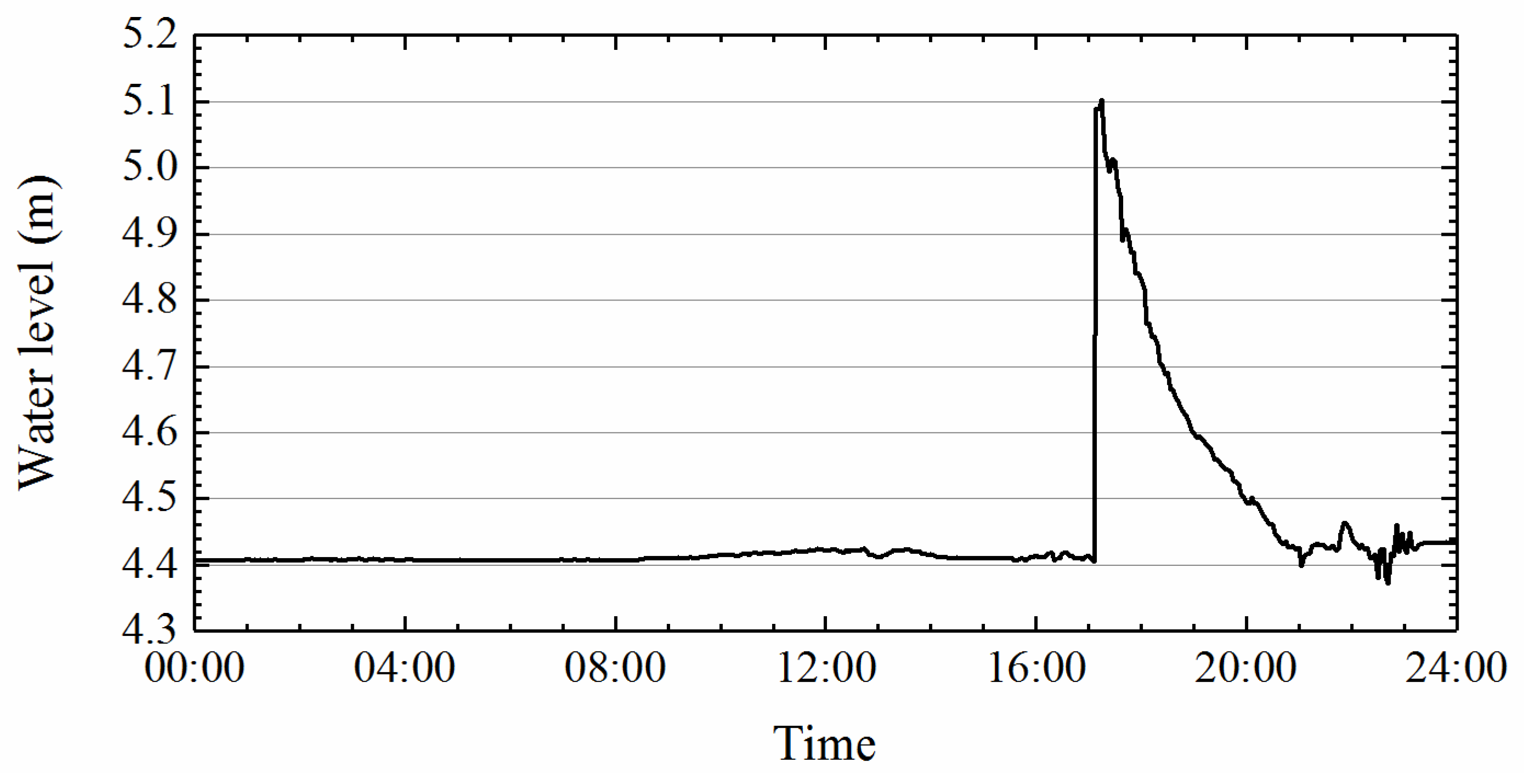
3.1. Field Measurements

In the present field investigations, the installed camera recorded the same water surface zone upstream of the elevated bridge where water level radar measurements were taken (Figure 1b,c). Figure 5 shows the water level measurements of the flash flood at wadi Samail, measuring the height of the water surface from a fixed previously known datum. The radar sensor emits short radar pulses toward the wadi bed to determine the water level. Based on a visual assessment of the stage hydrograph for the day of 28 October 2018, it is clear that over a duration of three hours, a sharp peak of flash flooding occurred after a long dry period. The rising stage of the flash flood was short, and the flood reached its peak stage in six minutes approximately. However, the recession stage occurred over more than two hours. During this period, the water level was decreasing and continuously fluctuating with an amplitude of 1 to 5 cm.

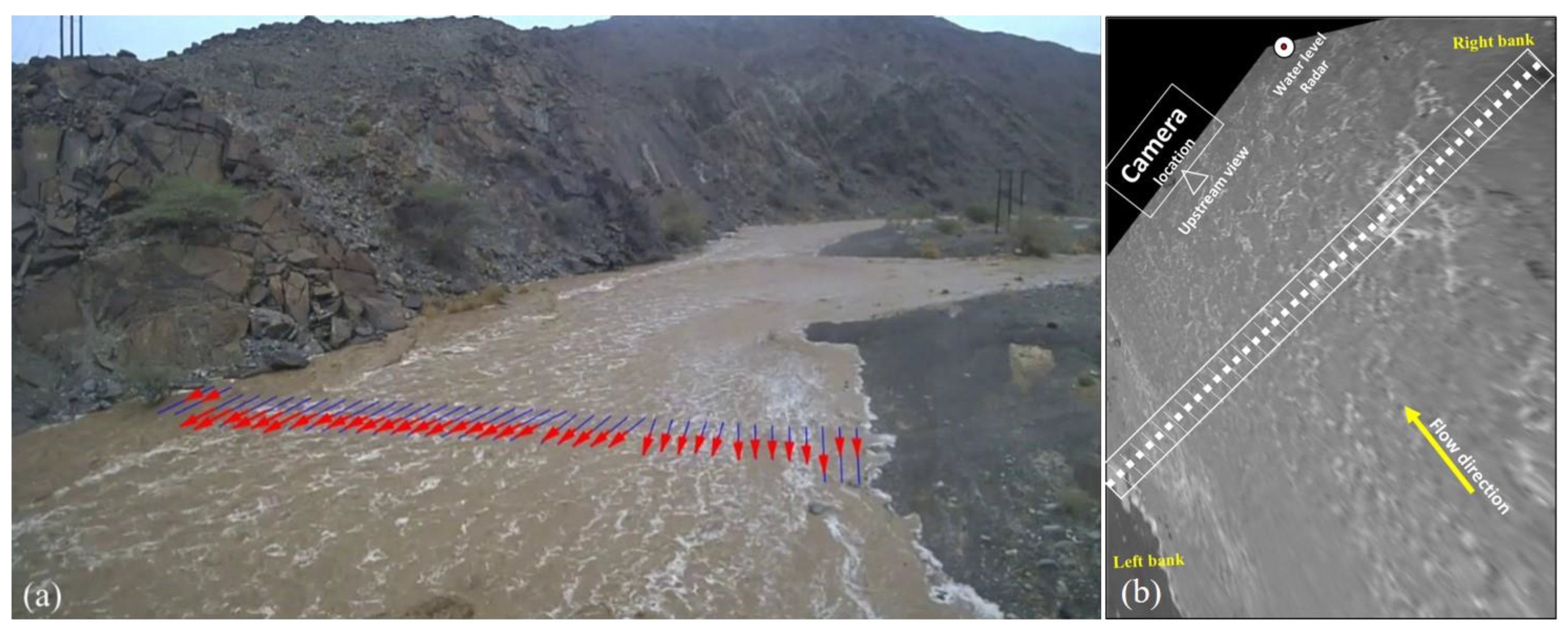
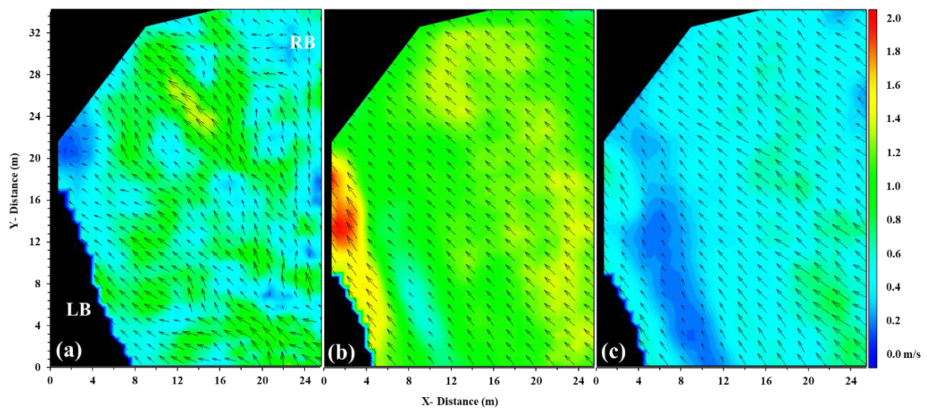
3.2. LSPIV Processing

Figure 6 illustrates the velocity vectors superimposed on the surface velocity magnitudes using LSPIV on 28 October 2018 for the wadi Samail flash flood. Because the wadi channel was flooded during the peak period, the width of the wadi was extended in the lateral flow direction when compared to the wadi width in the rising and falling periods. Figure 6a–c shows the averaged flow patterns with a velocity color map for the rising, peak, and recession limbs. The variation of surface velocity in each stage reflects the effects of the surface channel bed. The results of the LSPIV technique had the capability of providing good velocities distribution and show a 2-D flow pattern with an average time to detect movement and velocity. However, there were various sources of possible errors due to temporarily unclear natural tracer visibility in some areas based to the LSPIV analysis. Various sensitivity analyses for relevant parameters within the LSPIV analysis were conducted. Based on the actual measured slope area surveys and water levels for more than 10 years database and with regard to the slope area survey for the current flash flood event, the estimated velocities at the study site, we found the most accurate time-averaged flow velocity and then compared this with the velocities calculated using the STIV method.

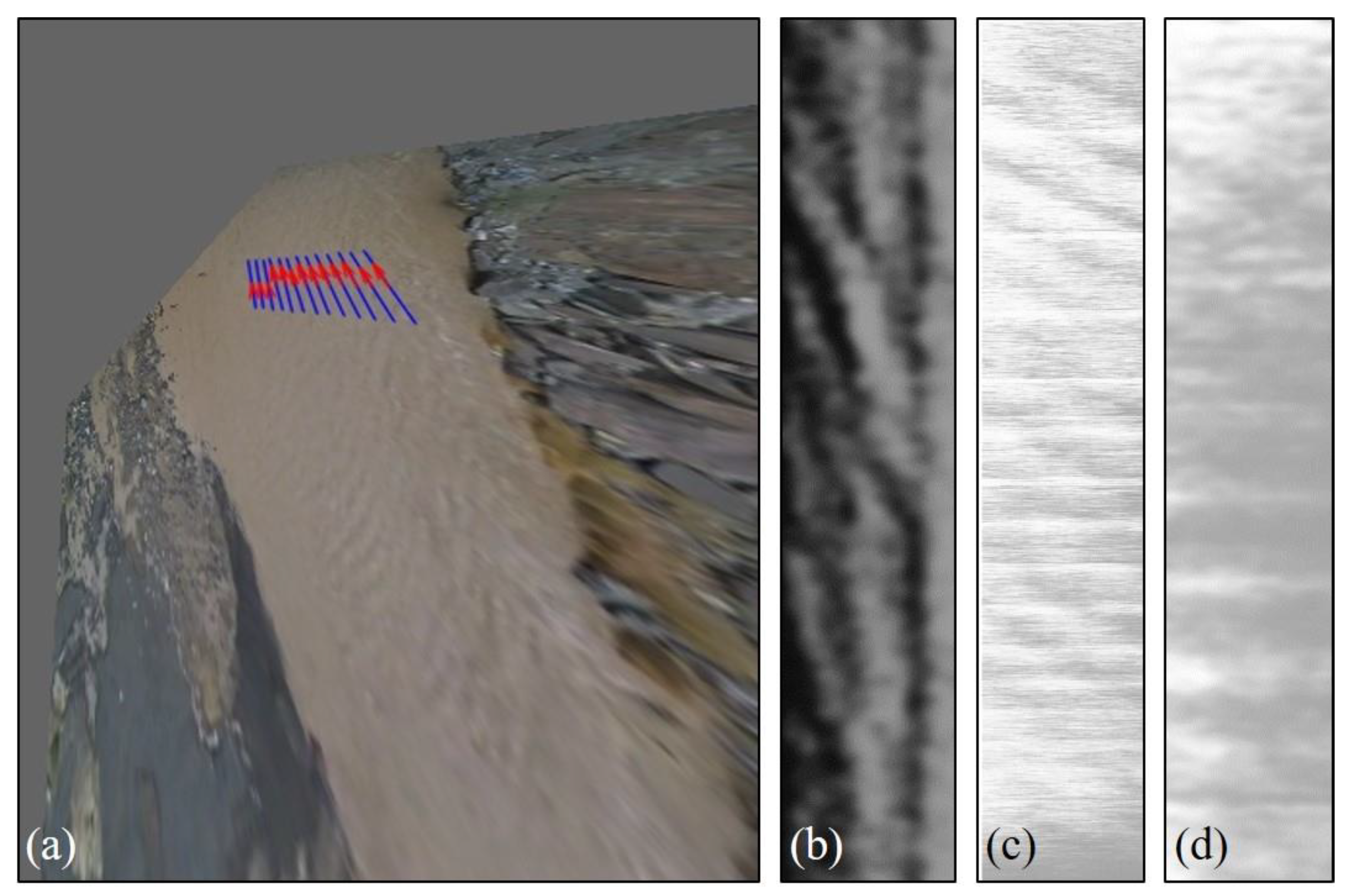
3.3. STIV Processing

The results analyzed by STIV are depicted in Figure 7b–d for three different periods of the recorded flood on 28 October 2018. The measured unidirectional velocity in Figure 7d is a sample calculation by STIV for purposes of comparison with the LSPIV method. A characteristic of a flash flood during high discharge is the large variation in the turbulence of the water surface, which, if detected, can improve the STIV analysis. Moreover, the morphology of the wadi channel beds comprising coarse materials causes hydraulic jumps and stationary waves [27]. The STIV showed obvious inclined brightness distribution patterns during the rising flood, peak, and recession (Figure 7b–d). However, the analysis of the rising and peak sections displays an almost linear texture. In addition, the results of the flow direction consisted of partially uniform patterns and texture between the peak and recession durations due to the decreasing surface turbulence and textures generated over the surface flow.

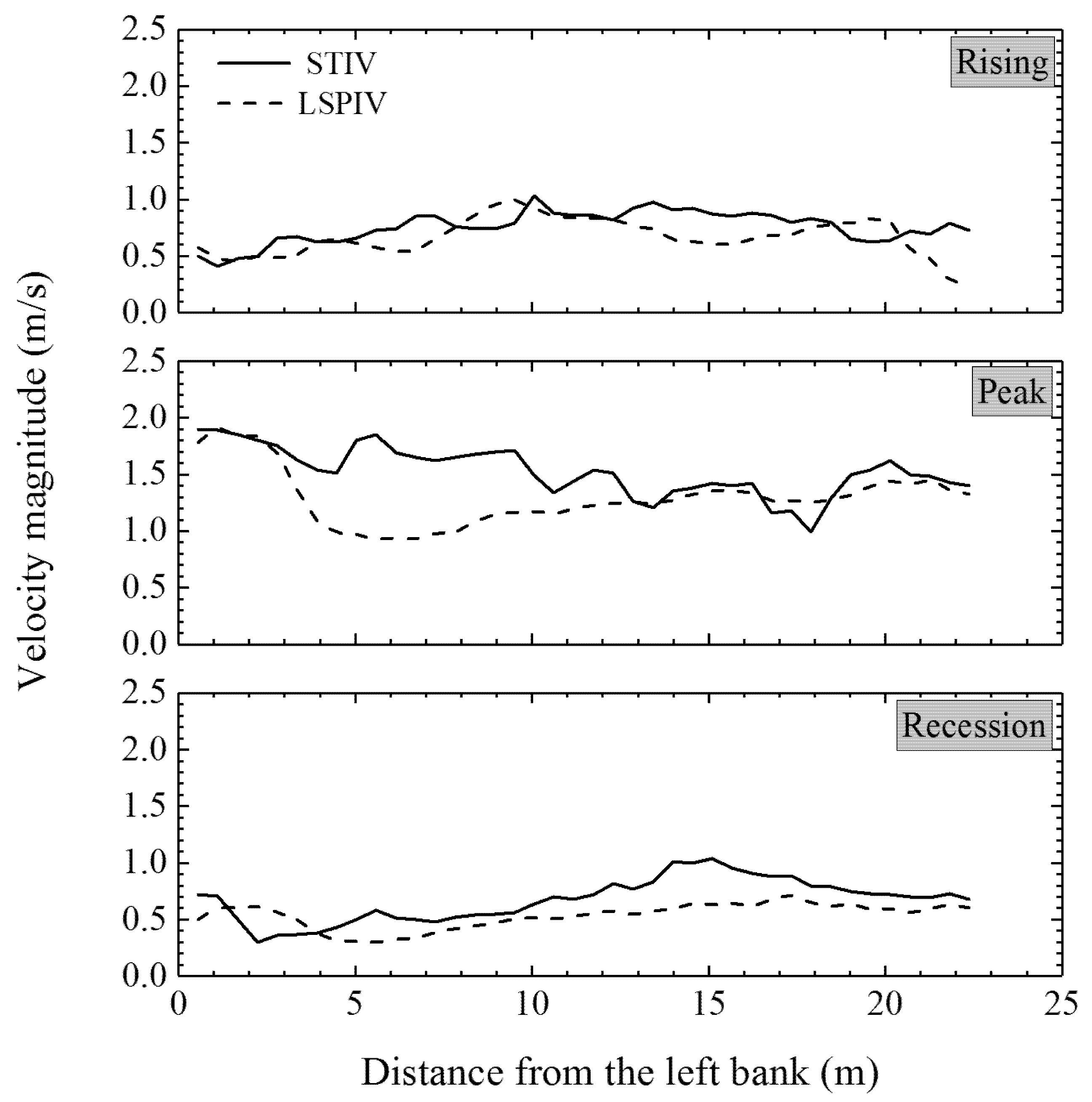
3.4. Comparison of Surface Flow Velocities Using Different Methods

The flow condition was extreme, and measuring it directly during the flash flood was dangerous due to large amounts of floating debris and its unknown velocity. Therefore, only water level measurements, which are local point measurements, can be utilized for wadi systems.

The field distribution of the mean surface velocity in the entire cross section, shown in Figure 4, computed by LSPIV and STIV techniques during the three stages is compared in Figure 8. The velocities estimated by STIV are generally higher than those estimated by LSPIV. The mean velocity in STIV during the rising phase was 0.76 m/s compared to LSPIV which was 0.69 m/s. The computed velocities of both techniques in the rising stage show a compatible trendline. It should be noted that the upstream of the computed zone include a large sand bar with vegetation, which causes bifurcation of the flow field, as can be seen in Figure 2a,b. The average velocities at the rising stage, measured by STIV and LSPIV, are in close agreement apart from values computed at 20 m from the left bank, where the mean velocity of STIV values are 11%, 17%, and 26% larger than those by LSPIV in the rising, peak and recession phase respectively.

In addition, the STIV values in the peak phase show a high velocity trend in the left bank compared to the LSPIV values; this is due to the shallow flow depths in this region, with mean cross-sectional velocities for STIV (1.5 m/s) and LSPIV (1.3 m/s). The high turbulence of surface flow increased the uncertainty of STIV values, rather than LSPIV values, in the peak stage [17]. Thereby, there were larger values of difference between the two techniques in this phase.

In the recession stages, however, the surface velocity displays continuous straight features with little disturbance and shows equivalent distribution between both methods. The surface velocities close to the right bank, where the channel bed is deeper, gradually increased toward the middle of the channel then decreased toward the left bank, except in the peak phase. The standard deviation of cross-sectional velocities between STIV and LSPIV in peak stage is about 0.2. In general, the mean surface velocity measurements and cross-sectional surface velocity results agree quite well between both methods. The analyzed images indicated that the mean flow velocities obtained at different times using LSPIV and STIV showed reasonable agreement, except for the peak limb values.

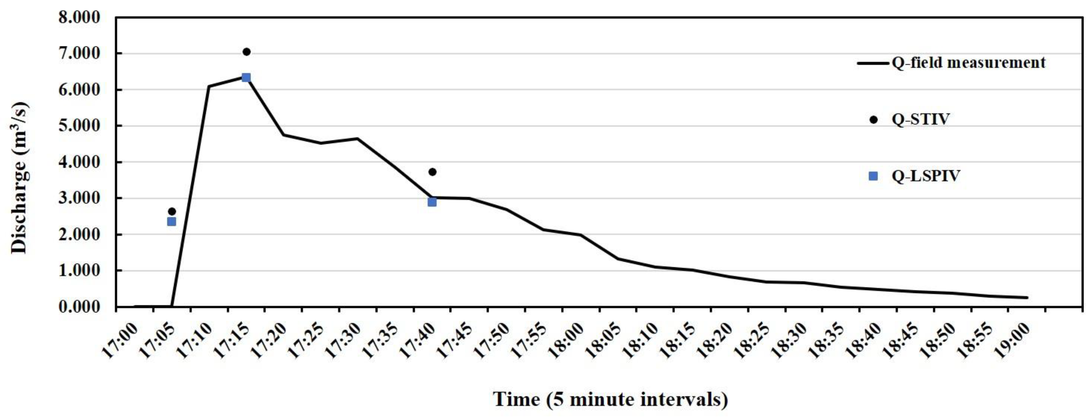
3.5. STIV and LSPIV Discharge Validation

Figure 9 displays the validation of a computed discharge hydrograph measured by a rating curve from slope–area methods (Q_m) and estimated discharges from the surface velocity distribution by LSPIV and STIV techniques. The results of the LSPIV and STIV were used to calculate the discharges (Q) with velocity area and average cross-sectional discharge (Q_avg). The discharge started to suddenly increase from 17:00, reached its peak at 17:15, and decreased again after that, becoming dry over a longer time period; this indicates the general characteristics of wadi flash floods in wadi systems. At the peak stage, the estimated discharges by LSPIV (about 6.48 m³/s) show very good agreement with the computed discharge from the slope–area method and cross-sectional average discharges (6.343 m³/s). Most of the values resulting from the two techniques are located within the same range of computed discharge from a similar cross-section of slope-area methods. In the rising limb, the values from LSPIV and STIV do not match with the field discharge measurements due to the faster rise of the discharge volume and its short duration.

However, the computed discharge from the slope–area method included many parameters that could give some reliable data. Thereby, the biggest finding from the data comparison was the power of using image-based methods as an alternative solution for improving water resource monitoring data in wadi systems.

4. Conclusions

In this paper, we presented the investigation of a real-time measurement method for wadi flash floods in arid regions using large scale particle image velocimetry (LSPIV) and space–time image velocimetry (STIV) techniques. We applied both techniques on videos recorded during the flash flood event on October 2018 at Wadi Samail in Oman, to quantify the flow discharges during different flow stages and we installed there four cameras on elevated bridges crossing a wadi channel due to the availability of field measurements, for example, water level radar and slope–area measurements. LSPIV and STIV techniques were deployed at the Al-Uqq gauging station in the wadi system.

A comparison of computed discharge values for surface velocity measurements using LSPIV and STIV techniques and the slope–area method was utilized to prove the effectiveness of these image-based techniques. The velocities measured by the LSPIV method are reliable and stable when there are high-resolution images after rectification with visible surface patterns. Despite their good performance, LSPIV and STIV techniques for the measurement of wadi flash floods in arid environments may still encounter uncertainties from various sources such as the ortho-rectification of an installed camera, sunlight reflectance, and surface velocity correction. All the measured results were in good agreement, with only small differences in the average velocities between the two techniques.

This research paper presents first-hand results for the enhancement of our scientific understanding of flash floods in arid environments. Recently, wadi hydrology has received increased interest from the scientific community. The current paper contributes to improving the monitoring and management of flash floods in wadi. Our investigations so far have only been of a medium-scale flash flood event. In conclusion, the application of LSPIV and STIV techniques should be extended to examine large-scale flows to check these potentially efficient methods for obtaining surface flow velocity and to make comparisons with field measurement velocities.

References

1. Al-Qurashi, A.; McIntyre, N.; Wheater, H.; Unkrich, C. Application of the Kineros2 rainfall–runoff model to an arid catchment in Oman. J. Hydrol. 2008, 355, 91–105. [Google Scholar] [CrossRef]
2. Al-Rawas, G.A.; Valeo, C. Issues with flash flood modeling in the capital region of Sultanate of Oman. In Geomatics Engineering; Schulich School of Engineering, University of Calgary: Calgary, AB, Canada, 2008. [Google Scholar]
3. Abdel-fattah, M.; Kantoush, S.A.; Saber, M.; Sumi, T. Rainfall-Runoff Modeling for extreme flash floods in Wadi Samail, Oman. J. JSCE 2018, 74, 691–696. [Google Scholar]
4. Tauro, F.; Selker, J.; van de Giesen, N.; Abrate, T.; Uijlenhoet, R.; Porfiri, M.; Manfreda, S.; Caylor, K.; Moramarco, T.; Benveniste, J.; et al. Measurements and Observations in the XXI century (MOXXI): Innovation and multi-disciplinarity to sense the hydrological cycle. Hydrol. Sci. J. 2018, 63, 169–196. [Google Scholar] [CrossRef]
5. Welber, M.; Coz, J.L.; Laronne, J.B.; Zolezzi, G.; Zamler, D.; Dramais, G.; Hauet, A.; Salvaro, M. Field assessment of noncontact stream gauging using portable surface velocity radars (SVR). Water Resour. Res. 2016, 52, 1108–1126. [Google Scholar] [CrossRef] [Green Version]
6. Tauro, F.; Petroselli, A.; Porfiri, M.; Giandomenico, L.; Bernardi, G.; Mele, F.; Spina, D.; Grimaldi, A.S. A novel permanent gauge-cam station for surface flow observations on the Tiber river. Geosci. Instrum. Methods Data Syst. 2016, 5, 241–251. [Google Scholar] [CrossRef]
7. Tauro, F.; Piscopia, R.; Grimaldi, S. Streamflow Observations From Cameras: Large-Scale Particle Image Velocimetry or Particle Tracking Velocimetry? Water Resour. Res. 2017, 53, 10374–10394. [Google Scholar] [CrossRef] [Green Version]
8. Adrian, R.J. Particle-imaging techniques for experimental fluid mechanics. Annu. Rev. Fluid Mech. 1991, 23, 261–304. [Google Scholar] [CrossRef]
9. Grant, I. Particle image velocimetry: A review. Proceedings of the Institution of Mechanical Engineers. Proc. Inst. Mech. Eng. C 1997, 211, 55–76. [Google Scholar] [CrossRef]
10. Lükő, G. Analysis of video-based discharge measurement method for streams. In Proceedings of the Scientific Students Associations Conference 2015, Pittsburgh, PA, USA, 8–11 October 2015. [Google Scholar]
11. Muste, M.; Fujita, I.; Hauet, A. Large-scale particle image velocimetry for measurements in riverine environments. Water Resour. Res. 2008, 44, W00D19. [Google Scholar] [CrossRef]
12. Fujita, I.; Muste, M.; Kruger, A. Large-scale particle image velocimetry for flow analysis in hydraulic engineering applications. J. Hydraul. Res. 1998, 36, 397–414. [Google Scholar] [CrossRef]
13. Sun, X.; Shiono, K.; Chandler, J.H.; Rameshwaran, P.; Sellin, R.H.J.; Fujita, I. Discharge estimation in small irregular river using LSPIV. Proc. Inst. Civ. Eng. Water Manag. 2010, 163, 247–254. [Google Scholar] [CrossRef] [Green Version]
14. Harpold, A.A.; Mostaghimi, S.; Vlachos, P.P.; Brannan, K.; Dillaha, T. Stream Discharge Measurement Using a Large-Scale Particle Image Velocimetry (LSPIV) Prototype. Trans. ASABE 2006, 49, 1791–1805. [Google Scholar] [CrossRef] [Green Version]
15. Sasso, S.F.D.; Pizarro, A.; Samela, C.; Mita, L.; Manfreda, S. Exploring the optimal experimental setup for surface flow velocity measurements using PTV. Environ. Monit. Assess. 2018, 190, 460. [Google Scholar] [CrossRef] [PubMed]
16. Koutalakis, P.; Tzoraki, O.; Zaimes, G. UAVs for Hydrologic Scopes: Application of a Low-Cost UAV to Estimate Surface Water Velocity by Using Three Different Image-Based Methods. Drones 2019, 3, 14. [Google Scholar] [CrossRef]
17. Fujita, I.; Watanabe, H.; Tsubaki, R. Development of a non-intrusive and efficient flow monitoring technique: The space-time image velocimetry (STIV). Int. J. River Basin Manag. 2007, 5, 105–114. [Google Scholar] [CrossRef]
18. Fujita, I.; Kitada, M.; Shimono, M.; Kitsuda, T.; Yorozuya, A.; Motonaga, Y. Spatial Measurements of Snowmelt Flood by Image Analysis with Multiple-Angle Images and Radio-Controlled ADCP. J. JSCE 2017, 5, 305–312. [Google Scholar] [CrossRef]
19. Marian, M.; Jochen, A.; David, A.; Robert, E.; Dennis, L.; Vladimir, N.; Colin, R. Velocity; Image-Based Velocimetry Methods. In Experimental Hydraulics: Methods, Instrumentation, Data Processing and Management, 1st ed.; CRC Press: London, UK, 2017; pp. 168–179. [Google Scholar]
20. Abdel-Fattah, M.; Kantoush, S.A.; Saber, M.; Sumi, T. Hydrological Modelling of Flash Flood in Wadi Samail, Oman; Kyoto University: Kyoto, Japan, 2016. [Google Scholar]
21. Piermattei, L.; Carturan, L.; Guarnieri, A. Use of terrestrial photogrammetry based onstructure-from-motion for mass balance estim ationof a small glacier in the Italian alps. Earth Surf. Process. Landf. 2015, 40, 1791–1802. [Google Scholar] [CrossRef]
22. Burns, J.; Delparte, D.; Gates, R.; Takabayashi, M. Integrating structure-from-motion photogrammetry with geospatial software as a novel technique for quantifying 3D ecological characteristics of coral reefs. PeerJ 2015, 3, e1077. [Google Scholar] [CrossRef]
23. Bird, S.; Hogan, D.; Schwab, J. Photogrammetric monitoring of small streams under a riparian forest canopy. Earth Surf. Process. 2010, 35, 952–970. [Google Scholar] [CrossRef]
24. Kantoush, S.A.; Schleiss, A.J. Large-scale PIV surface flow measurements in shallow basins with different geometries. J. Vis. 2009, 12, 361–373. [Google Scholar] [CrossRef]
25. Coz, J.; Hauet, A.; Pierrefeu, G.; Dramais, G.; Camenen, B. Performance of image-based velocimetry (LSPIV) applied to flash-flood discharge measurements in Mediterranean. J. Hydrol. 2010, 394, 42–52. [Google Scholar] [CrossRef]
26. Haue, A.; Creutin, J.-D.; Belleudy, P. Sensitivity study of large-scale particle image velocimetry measurement of river discharge using numerical simulation. J. Hydrol. 2008, 349, 178–190. [Google Scholar]
27. Grant, G.E. Critical flow constrains flow hydraulics in mobile-bed streams: A new hypothesis. Water Resour. Res. 1997, 33, 349–358. [Google Scholar] [CrossRef] [Green Version]
Figure 1. (a) Photo of the inclined camera installed on an elevated bridge crossing the wadi. (b) Photo of the water level radar station. (c) Location of Wadi Samail showing topographic elevation and the locations of the cameras and the water level radar.
Hydrology 06 00027 g001
Figure 2. (a) View of the rising flash flood. (b) View of the flash flood peak. (c) Photogrammetric image of the wadi channel bed showing the locations of the ground reference points (GRPs), camera, and water level radar.
Hydrology 06 00027 g002
Figure 3. Flowchart of the flow monitoring and analysis system.
Hydrology 06 00027 g003
Figure 4. (a) The computed cross-sectional zone with the search line used in space–time image velocimetry (STIV); (b) Ortho-rectified image showing the location of cross-sectional of computed surface flow velocity by large-scale particle image velocimetry (LSPIV).
Hydrology 06 00027 g004
Figure 5. Water level measurements, 4.4 m elevation of the channel bed, on 28 October 2018 recording the three flash flood phases at the study area.
Hydrology 06 00027 g005
Figure 6. Images (a), (b), and (c) show the average flow patterns with velocity color maps using LSPIV for the rising, peak, and recession limbs, respectively, of flooding on 28 October 2018, left bank (LB), right bank (RB).
Hydrology 06 00027 g006
Figure 7. (a), (b) and (c) Space–time images of a search line during rising, peak, and recession, respectively. (d) Measured surface flow velocity using space–time image velocimetry (STIV) with rectification during the 28 October 2018 flood recession.
Hydrology 06 00027 g007
Figure 8. Comparison of cross-sectional surface velocities measured by LSPIV and STIV for the three flood stages.
Hydrology 06 00027 g008
Figure 9. Validation of space–time image velocimetry (STIV)- and large-scale particle image velocimetry (LSPIV)-computed discharge from surface flow velocities and discharge computed from water levels.
Hydrology 06 00027 g009