Estimation of Water Balance and Nitrate Load in the Upper Basin of Aguascalientes, Mexico, Using SWAT

Abstract

Intensive agriculture in semi-arid watersheds is considered a threat to global water security; however, the hydro-agronomic mechanisms that control diffuse pollution sources are often insufficiently characterized at the watershed scale. This study evaluates the hydrological response and nitrate leaching dynamics in the Upper Aguascalientes watershed by implementing the SWAT model, forced with meteorological data and calibrated using runoff derived from ERA5 reanalysis. Methodologically, the Potential Nitrate Leaching Risk Index (IRP_N) was formulated and coupled to the hydrological results. The comparative analysis shows that ERA captures the temporal dynamics of the HRUs, although it tends to significantly overestimate runoff volumes. The basin exhibits a marked scale-dependent duality, with the upper zone operating under a Hortonian regime, while the lower basin exhibits attenuation at the basin scale due to spatial integration and distributed storage processes. The $\left(IR{P}_N\right)$ analysis demonstrates a critical disconnect between fertilization rates (>1300 kg N·ha⁻¹) and crop absorption capacity, turning excess nitrogen into a rapid transport vector during runoff events. Finally, the results underscore the need to complement water management and infrastructure strategies with technical training programs and regulatory frameworks that promote modern agricultural practices aligned with the system’s retention capacity.

1. Introduction

Water scarcity represents a critical challenge at the global level, particularly in semi-arid regions where limited precipitation and high evapotranspiration rates restrict water availability [1,2,3]. These regions are especially vulnerable to anthropogenic pressures from agricultural intensification, urbanization, and industrial development, which increase water demand and degrade water quality through contaminant discharge [4,5,6]. In agricultural systems, excessive application of nitrogen fertilizers promotes nutrient leaching into surface and groundwater, leading to eutrophication and contamination of water bodies [7,8,9,10]. This process intensifies in watersheds dominated by intensive agriculture and irrigation systems [11,12,13].

Diffuse pollution has received increasing scientific attention due to the complexity of identifying non-point sources, which complicates both its assessment and management [3]. This problem is particularly critical for the transport of nitrogen (N) from agricultural lands to water bodies, due to exhibit high mobility through surface runoff and subsurface flow. Mexico, facing not only an imminent water-scarcity crisis but also a severe problem of diffuse contamination. The North-Central region is experiencing recurrent droughts and growing limitations in water availability, conditions that directly affect the use of its hydrological systems and intensify the vulnerability of its basins [1,2,4].

Aguascalientes is part of North-Central Mexico, where nearly 70% of the state’s agricultural production is concentrated in the northern region. In particular, the municipalities of Pabellón de Arteaga, Rincón de Romos, and Tepezalá are among the main producers of corn and beans in the state. This intensive activity requires the use of a high among of nitrogen fertilizers and water to maintain the crops productivity. Also, factor as irregular annual rainfall and near-total dependence on groundwater, have led to the progressive overexploitation of aquifers [1,4,5], a phenomenon that reflects the depletion of groundwater reserves documented globally in zones of intensive agriculture [6,7,8,9,10].

On the other hand, hydrological models provide a useful framework for evaluating water balance components and simulating contaminant transport processes at the watershed scale. Among these tools, the Soil and Water Assessment Tool (SWAT) have been widely applied to represent hydrological processes and nutrient transport in agricultural basins [14,15,16,17,18,19,20]. SWAT is a physically based, semi-distributed model that simulates watershed processes through hydrological response units, under different land-use and management conditions. Its robustness and capacity to represent agricultural practices have made it one of the most widely used tools for evaluating non-point source pollution in agricultural environments [11].

However, hydrological modeling in semi-arid regions often faces limitations related to sparse hydrometric monitoring networks. In such contexts, climate reanalysis datasets provide an alternative source of atmospheric information to drive hydrological simulations. The ERA5 reanalysis dataset offers high-resolution climate variables that enable hydrological analyses in poorly gauged basins and has been increasingly adopted in watershed modeling studies. Recent research demonstrates that integrating ERA5 with hydrological models can provide reliable estimates of runoff dynamics in data-scarce environments [12]. In addition, empirical data obtained directly from farmers provide valuable information on fertilizer application rates, cropping systems, and management practices that influence nitrate mobilization, that influence nitrate mobilization, improving the understanding and identification of potential sources of diffuse pollution.

Therefore, SWAT model was selected for its ability to simulate hydrological processes and nutrient transport under semi-arid conditions, particularly where continuous discharge records are limited. Meteorological forcing and runoff information derived from the ERA5 reanalysis dataset supported model evaluation. Furthermore, estimating a Potential Nitrate Leaching Risk Index (IRP_N) can provide an independent empirical assessment of the intensity of agricultural management in arid regions, as well as characterize the spatial patterns of fertilizer use and identify areas with high potential for nitrate leaching. This approach represents a viable alternative for estimating possible non-point sources of contamination and supports a broader interpretation of diffuse contamination processes in semi-arid agricultural watersheds.

This study has two main objectives: (i) estimate the water balance and characterize nitrate loads in the upper Aguascalientes basin using hydrological modeling, and (ii) estimate potential nitrate risk associated with agricultural practices through the IRP_N index. This work improves understanding of hydrological and agricultural drivers of nitrate transport in semi-arid basins and provides information to support more effective water management strategies.

2. Materials and Methods

2.1. Study Area

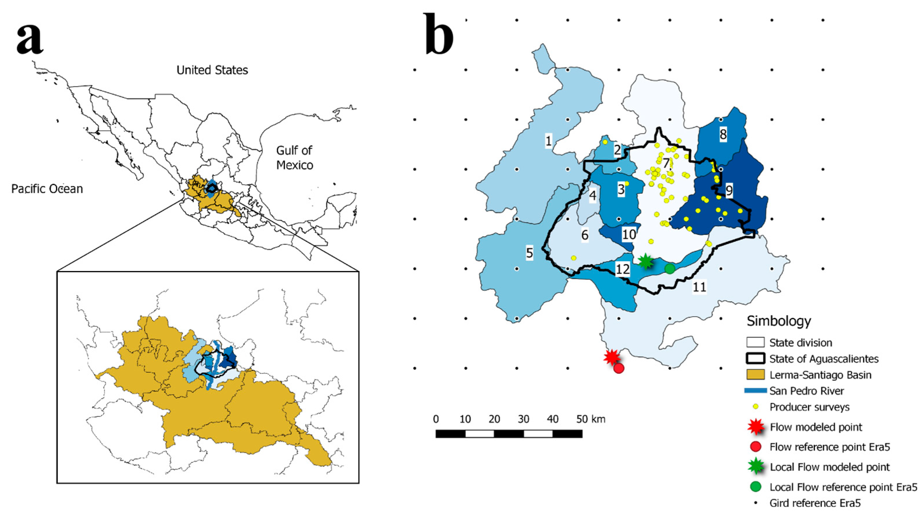
In Mexico, water management is organized into 37 hydrological regions (Figure 1a). These regions are delineated based on natural watershed boundaries, which do not necessarily coincide with political divisions such as states or municipalities. The watershed serves as the fundamental unit for water management [13]. The state of Aguascalientes lies entirely within Hydrological Region VIII, Lerma–Santiago–Pacific, and more specifically within the Alto Santiago subregion (Figure 1a). The study area focuses on the upper basin of the San Pedro River. While the agronomic characterization centers on the intensive agricultural district of Pabellón de Arteaga (where survey data was collected), the hydrological analysis integrates the basin response at the El Niágara Dam (102°22′16″ W, 21°46′45″ N), a strategic control point located 3 km southwest of Aguascalientes City. This dam regulates the main channel of the San Pedro River, capturing the runoff from the high-intensity agricultural zones upstream.

Figure 1b shows the state of Aguascalientes along with the neighboring state boundaries and the official sub-basin divisions defined by Comisión Nacional del Agua [13]. For this study, the gauging and calibration point was established at basin flow measurement point (basin outlet). This infrastructure represents the hydrological outlet of the studied agricultural system. At this point, the measured discharge reflects the cumulative hydrological response of the entire upstream area, integrating the flows from the agricultural municipalities before they enter the urban zone. These observed flow data were used for model calibration, which aims to minimize the difference between the simulated and observed streamflow generated by SWAT.

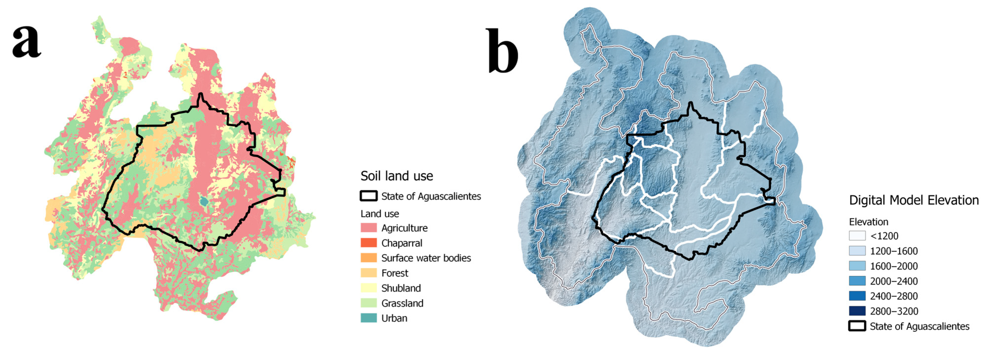
The physical characteristics of the basin that determine its hydrological response are presented in Figure 2. Figure 2a illustrates the spatial distribution of land use, showing that agriculture clearly dominates the central valley, which geographically coincides with the location of the surveyed producers (see Figure 1b) and represents the primary source of nutrient loading to El Niágara reservoir. The higher-elevation zones to the west are primarily covered by scrubland, grassland, and forest. Figure 2b displays the Digital Elevation Model (DEM), which reveals a relief with a pronounced west–east gradient. The highest elevations, exceeding 2800 m a.s.l., occur in the western mountain ranges, whereas the lowest areas (1200–1600 m a.s.l.) are located in the central valley, where the San Pedro River flows.

2.2. Hydrological Model

The semi-distributed hydrological model SWAT (Soil and Water Assessment Tool), developed by the USDA Agricultural Research Service (ARS), was used for this study [23,24]. This model simulates hydrological and biogeochemical processes at daily or monthly time steps, integrating water flows, sediment transport, and nutrient dynamics under various land uses [25]. SWAT was selected due to its widespread validation and robustness in simulating hydrological processes and non-point source pollution in agricultural watersheds, particularly in semi-arid regions.

The water balance is the core of SWAT’s hydrological component, calculated for each hydrological response unit (HRU) daily based on the following equation:

$$S{W}_t=S{W}_o+{\displaystyle \sum _{i=1}^t{\left(R_{day}-Q_{surf}-E_a-W_{seep}-Q_{gw}\right)}_i}$$

(1)

where $S{W}_0$ and $S{W}_t$ are the soil water content at the beginning and end of the period, respectively; $R_{day}$ is precipitation; $Q_{surf}$ is surface runoff; $E_a$ is evapotranspiration; $W_{seep}$ is the volume of water percolating into the vadose zone; and $Q_{gw}$ is baseflow. All variables are expressed in millimeters and refer to day $i$.

The hydrological simulation was driven by daily precipitation and temperature data. The year 2020 was used as a spin-up (warm-up) period to stabilize the model’s initial conditions. Hydrological calibration focused on key parameters, including the curve number $\left(C{N}_2\right)$, available soil water content (SOL_AWC), and the soil evaporation compensation factor (ESCO). Calibration adjustments consisted of a +12.5% relative increase in CN₂ and a −5% relative decrease in SOL_AWC applied uniformly across the basin. The soil evaporation compensation factor (ESCO) assigned a value of 0.8 within its recommended range. Parameter bounds were maintained within the default SWAT+ limits. These adjustments aimed to improve the representation of seasonal runoff dynamics rather than site-specific parameter optimization.

The model implementation used QGIS (v3.4.11) with the QSWAT+ plugin (v1.2.2) and SWAT+ (v1.2.2). Surface runoff was computed using the SCS Curve Number (CN) method. Potential evapotranspiration estimation used the Penman–Monteith method. Channel routing performed using the Muskingum routing method. Channel transmission losses remained at default settings (CH_K2 = 0), meaning that no explicit infiltration from channels received parameterization. Therefore, any buffering behavior discussed in the results primarily reflects soil water storage and shallow groundwater processes represented within SWAT+, rather than channel transmission losses. Nitrate in surface runoff obtained from the SWAT+ output variable SURQ_NO3, which represents nitrate mass transported in surface runoff at the HRU level. This variable is expressed as a real load (kg·ha⁻¹ per time step), not a concentration. The “specific nitrate load (kg·ha⁻¹)” reported in this study directly corresponds to this output.

2.2.1. Input Data

The model parameterization used three main categories of input data: geospatial, meteorological, and management/calibration datasets.

Spatial datasets defined the physical structure of the watershed. Land use and vegetation cover (LULC) data were obtained from CONABIO’s National Inventory Series IV and V [13], corresponding to the distribution shown in Figure 2a. These LULC categories were standardized to the USGS Global Land Cover Characterization (GLCC) classification system to ensure compatibility with the SWAT database. Topography was derived from a 15 m-resolution Digital Elevation Model (DEM) provided by INEGI (National Elevation Continuum Series I) [22], which delineates the basin’s relief and gradient (Figure 2b).

QSWAT+ defined the Hydrologic Response Units (HRUs) by overlaying land use, soil type, and slope classes. No threshold filtering was applied (0% for land use, soil, and slope), ensuring that all spatial heterogeneity remained preserved in the model configuration. Discretization divided slope into four classes: 0–3%, 3–5%, 5–10%, and >10%. The final model configuration resulted in 158 sub-basins and 3099 HRUs. No additional merging or filtering of HRUs occurred after delineation; all generated HRUs were retained to preserve spatial detail.

Daily precipitation and maximum and minimum temperature from the ERA5 reanalysis [26] used as meteorological forcing. For the SWAT parameter adjustment, the hydrological outlet of the basin (corresponding to sub-basin 11, Figure 1b, star symbol) defined as the point of interest. Since no observed discharge records were available at the basin outlet, daily surface runoff from the ERA5 [26] was used as a proxy reference series. The surface runoff variable (ro), expressed as equivalent water depth (m), was extracted from the ERA5 grid cell whose centroid is geographically closest to the outlet coordinates. Given the coarse native spatial resolution of ERA5 (~0.25°), this grid cell represents a regional-scale hydrological signal rather than an exact basin-averaged discharge. No bias correction was applied due to the absence of in situ discharge observations. Daily ERA5 data were retrieved directly at daily resolution and converted to mm day⁻¹ for comparison with SWAT-simulated surface runoff. As illustrated in the revised Figure 1b, the selected ERA5 grid cell corresponds to the nearest reference point to the basin outlet. Given that ERA5 runoff was used to capture temporal variability rather than exact discharge magnitudes, minor spatial discrepancies in grid-cell selection are not expected to substantially influence the parameter adjustment procedure. Consequently, ERA5 surface runoff was used to guide parameter adjustment by matching the temporal variability and seasonality of simulated flows, and the resulting time series was used to adjust CN₂, SOL_AWC, and ESCO.

To define management scenarios, empirical information was collected through surveys conducted with 134 local farmers (Figure 1b, yellow dots). These surveys provided detailed parameters on nitrogen fertilizer application (rate, type, and frequency) and soil management practices. Two management scenarios were defined. The control scenario consisted of zero fertilizer and pesticide applications, representing a baseline condition without external nutrient inputs. The active fertilization scenario implemented a single fertilizer application at sowing for corn HRUs using the survey-derived rates reported in Section 3.3. No other hydrological or climatic parameters were modified between scenarios.

2.2.2. Model Evaluation

Model performance was evaluated using standard statistical metrics commonly applied in SWAT studies [14,15]: the coefficient of determination R², Nash–Sutcliffe efficiency (NSE), percent bias (PBIAS), and the RMSE-observations standard deviation ratio (RSR). The resulting performance was classified as “very good,” “good,” “satisfactory,” or “unsatisfactory” based on the established guidelines for watershed models [23].

The coefficient of determination R² describes the proportion of variance in the observed data that is explained by the model [24]. R² values range from 0 to 1, with higher values indicating better model performance [23]. The NSE is a normalized statistic that determines the relative magnitude of the residual variance compared to the observed data variance [18]. NSE ranges from $\infty$ to 1. An NSE value of 1 indicates a perfect match, while values between 0 and 1 are generally considered acceptable predictive performance [16]. The PBIAS measures the average tendency of the simulated data to be larger or smaller than the observed data. A PBIAS of 0 indicates an accurate simulation. Positive values indicate model overestimation bias, while negative values indicate underestimation bias [16,19,20]. Finally, the RSR was used to standardize the root mean square error using the standard deviation of the observations. RSR values range from 0 to a large positive number, with lower values indicating better model performance. According to [16], RSR ≤ 0.50 is classified as “Very good,” 0.50–0.60 as “Good,” 0.60–0.70 as “Satisfactory,” and >0.70 as “Unsatisfactory.”

2.3. Statistical Analysis of Empirical Data

An exploratory statistical analysis was performed on the agricultural data obtained from the 134 farmer surveys, conducted through random sampling across different municipalities between July and August of 2025. The survey collected categorical (crop type, irrigation system, fertilizer type, and nitrogen and potassium source) and numerical variables (application rates, frequencies, and cultivated plot area). Agrochemicals were grouped according to their active ingredients. To mitigate the influence of extreme outliers in the survey responses, a 1% trimmed mean (mean, trim = 0.01) was used as a robust measure of central tendency [27]. Standard deviations and 95% confidence intervals were also calculated using bootstrap resampling techniques.

To ensure data quality, filters were applied to exclude observations outside of realistic operational ranges and supported by recent studies: fertilizers (≤1000 kg · ha⁻¹), potassium sources (≤400 kg · ha⁻¹ and ≤6 applications), insecticides (≤16 L · ha⁻¹ and ≤8 applications), and herbicides (≤15 L · ha⁻¹ and ≤5 applications) [28,29]. After applying these criteria, the final dataset used for subsequent analyses consisted of 99 observations. To standardize application rates, herbicide and pesticide doses were normalized using a reference dilution of 1 L per 200 L of water. This statistical treatment was strictly descriptive and aimed at organizing and preparing the empirical data for hydrological model parameterization and subsequent risk assessment analyses. The trimmed mean values of fertilizer application rates and application frequencies, as well as the fertilizer types identified in the surveys, defined the agricultural management inputs used in the SWAT model. All analyses were implemented in the R programming language v 4.5.0 [30].

2.4. Geospatial Modeling and Nitrate Leaching Risk Assessment

To characterize agricultural management practices and evaluate their potential contribution to diffuse nitrate pollution, an integrated analytical framework was developed combining descriptive geocoding for geographic visualization, a literature-based multi-criteria risk index (IRP_N), and unsupervised multivariate techniques (MCA–HCPC). This framework was designed to identify structurally coherent management typologies and assess their associated nitrate leaching risk without relying on explicit spatial statistical modeling.

2.4.1. Geocoding and Data Processing

The spatial component of the analysis was built upon a dataset of 99 unique agricultural localities identified through the surveys. As the primary data lacked explicit geospatial coordinates, a batch geocoding process was executed within the R programming environment (v4.5.0 [30]). The tidygeocoder package (v1.0.5 [31]) was used to query the OpenStreetMap Nominatim API.

Prior to querying, toponyms were standardized following the pattern “Locality, Municipality, State” to maximize retrieval accuracy. The resulting coordinates (geographic centroids in the WGS84 system) were validated and integrated into the master database, enabling explicit spatial linkage between the recorded agricultural practices and the physical vulnerability of the study area. Survey data included locality names but not plot-level coordinates. Geographic positions were therefore assigned using OpenStreetMap (Nominatim) to obtain locality centroids. Because subsequent analyses were conducted at the HRU and sub-basin scales, centroid-based positional uncertainty does not materially affect hotspot identification or monitoring network design.

2.4.2. Potential Nitrate Leaching Risk Index IRP_N

A synthetic index called the Potential Nitrate Leaching Risk Index (IRP_N) was constructed to quantify the relative susceptibility of each location to generate diffuse nitrate pollution. The index follows a weighted additive structure grounded in literature-based risk attribution rather than process-based simulation, integrating nine management and site-related variables. For each location, IRP_N is calculated as follows.

$$IR{P}_N={\displaystyle \sum _{i=1}^n\left(v_{ij}\cdot W_i\right)}$$

(2)

where $v_{ij}$ is the ordinal risk score (0–3) assigned to variable $i$ at location $j$, (0 = Null, 3 = High); $W_i$ is the weighting coefficient and $n=9$ is the total number of variables [6,28]. The complete scoring rubric, including category definitions as well as threshold criteria, is provided in Table S1 in Supplementary Materials.

The weighting scheme (

Table 1. Weighting factors $W_i$ for agricultural variables used in the Potential Nitrate Leaching Risk Index $IR{P}_N$.

Risk Contribution	$\mathbf{Weight}\left({\mathit{W}}_{\mathit{i}}\right)$	Management Variable
High	0.345	Fertilizer Type
High	0.345	Fertilizer Application Rate
Moderate	0.145	Irrigation Method
Low	0.075	Crop Type
Low	0.05	Fertilizer Application Frequency
Negligible	0.015	Potassium Source
Negligible	0.015	Potassium Application Rate
Negligible	0.01	Potassium Application Frequency
Null	0	Cultivated Area

) assigned 69% of the total weight to fertilizer type and nitrogen application rate, considering the influence of nitrogen input intensity on nitrate leaching across cropping systems.

Highly soluble N forms and excessive application rates increase nitrate mobility [6,32], while irrigation practices modulate percolation dynamics [28,33]. Crop-related weighting accounts for differences in nitrogen uptake efficiency [34]. This structure is consistent with environmental composite index methodologies that prioritize direct pressure variables [35].

Although cultivated area was evaluated, it was assigned a weight of zero due to insufficient consistent evidence linking field size directly to nitrate leaching risk [36]. Nevertheless, it was retained in the multivariate analysis (Section 2.4.3) to support structural characterization of management clusters [37]. For interpretative purposes, IRP_N values were classified into three ordinal risk categories based on predefined thresholds: Low Risk (IRP_N ≤ 1.0), Medium Risk (1.0 < IRP_N ≤ 2.0), and High Risk (IRP_N > 2.0). These thresholds were established to ensure consistent categorical differentiation across the theoretical range of the composite index (0–3) while preserving interpretability and avoiding over-fragmentation of risk classes [38].

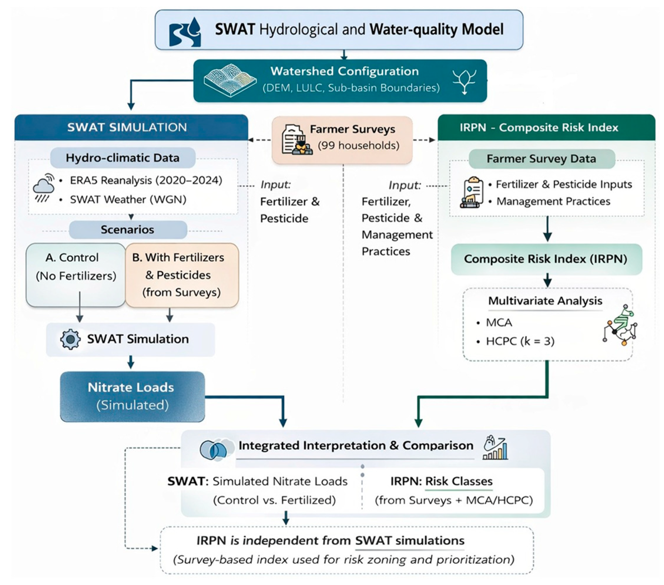
The IRP_N was constructed independently from the SWAT simulations and was derived exclusively from farmer survey data describing fertilizer use, pesticide application, and management practices. The SWAT model used survey information solely to define fertilization inputs under Scenario B (agricultural management), but the IRP_N itself did not incorporate SWAT-simulated nitrate loads or hydrological outputs. Thus, both analytical components were developed in parallel and integrated only at the interpretation stage as shown in Figure 3.

2.4.3. Multivariate Analysis: MCA and HCPC

To identify spatial patterns of agricultural management and associated risk without introducing priori assumptions, an unsupervised multivariate framework was implemented using the FactoMineR package (v2.11) in R. Given the predominantly categorical structure of the dataset, algorithms reliant on simple Euclidean distances were precluded in favor of a robust sequential strategy. The analysis commenced with a Multiple Correspondence Analysis (MCA), which functioned as a critical feature extraction step. This technique transformed the original categorical variables into a continuous factorial space defined by principal dimensions, allowing the preservation of the main sources of variability and the representation of associations among management categories in a reduced metric space.

Subsequently, Hierarchical Clustering on Principal Components (HCPC) was applied to the individual factorial coordinates obtained from the MCA. Clustering was performed using Ward’s minimum inertia criterion, producing a dendrogram that partitions observations into a set of internally homogeneous clusters while maximizing between-cluster variance. This combined MCA–HCPC framework enabled the identification of latent structural patterns in the data, grouping agricultural localities according to similarities in management practices and associated risk profiles. The resulting clusters provided an empirical basis for distinguishing contrasting levels of potential nitrate leaching risk, derived exclusively from the intrinsic multivariate structure of the dataset.

The MCA-HCPC framework was implemented as an exploratory data-structuring approach to identify latent management patterns and assess internal coherence among survey variables. It does not constitute a predictive model and does not modify or calibrate the hydrological simulations. However, an extended version of this analysis is provided in the Supplementary Materials for the reader’s reference.

2.4.4. Validation and Stability of the Multivariate Structure and IRP_N Interpretation

The robustness of the analytical framework was assessed using a validation strategy summarized in

Table 2. Model validation and cluster stability assessment criteria for the MCA-HCPC approach.

Statistical Interpretation Criteria	R Package v 4.5.0/ Formula	Objective	Method	Validation Indicator
Statistical Interpretation Criteria	FactoMineR (v2.11)	Quantify total variance explained by principal dimensions.	MCA	Explained Inertia
Higher inertia indicates better capture of variable associations [37].	FactoMineR (v2.11)	Identify influential categories for axis construction.	MCA	Variable Contributions
High contributions indicate key drivers in axis formation [37].	FactoMineR (v2.11)	Measure representation quality of variables on axes.	MCA	Squared Cosine (cos2)
${\cos }^2>5$ indicates reliable representation [39].	${\chi }^2=\mathrm{Inertia}\times N$	Test global dependence between variables.	MCA	Global Chi-squared
$p-\mathrm{value}<0.05$ justifies MCA application [40].	FactoMineR (v2.11)	Measure quality of observation projection.	MCA	Individual (cos2)
${\cos }^2>5$ indicates strong representation of individuals [40].	FactoMineR (v2.11)	Assess robustness to subsampling.	MCA	Cross-validation
Correlations > 0.85 suggest robust factor structure [40].	FactoMineR (v2.11) + cluster	Test clustering reproducibility under resampling.	HCPC	Bootstrap + ARI
ARI > 0.6 validates clustering stability [41].	Cluster	Evaluate cluster compactness and separation.	HCPC	Average Silhouette

. For the Multiple Correspondence Analysis (MCA), representation quality was evaluated using explained inertia and squared cosine (cos²) metrics, which quantify how effectively the retained dimensions capture variability and associations among categorical variables. These metrics were used exclusively to assess the adequacy of the factorial space for subsequent analyses, without imposing absolute representation thresholds.

Cluster stability was then evaluated within the Hierarchical Clustering on Principal Components (HCPC) procedure using bootstrap resampling and the Adjusted Rand Index (ARI), enabling the assessment of the reproducibility and internal consistency of the unsupervised partitioning. Finally, the Potential Nitrate Leaching Risk Index (IRP_N) was examined in relation to the resulting cluster structure. Differences in IRP_N values among clusters were analyzed descriptively to evaluate their interpretative coherence with the multivariate segmentation, thereby providing an internal consistency check between the expert-based index formulation and the data-driven patterns identified by the MCA–HCPC framework.

The overall methodological structure is summarized in Figure 3.

As illustrated in Figure 3, the SWAT-based process simulation and the IRP_N framework represent parallel analytical components. While survey data informed fertilizer inputs for SWAT scenario simulations, the IRP_N was derived independently from survey variables and analyzed through MCA-HCPC. The integration of both components occurred exclusively during the interpretative comparison phase.

3. Results

3.1. Model Assessment

Hydrological model calibration and validation were carried out by comparing simulated surface runoff against ERA5 discharge data at basin outlet (Figure 1b, red star). A one-year spin-up period (2020) was implemented to stabilize the model’s initial conditions. Figure 3 presents the visual comparison of the mean monthly runoff hydrograph. The calibration period covered 2021–2022, while the validation period spanned 2023–2024. Quantitative performance was evaluated using the statistical indicators R², NSE, PBIAS, and RSR (

Table 3. Statistical indicators assessing the performance of the SWAT model during the calibration and validation periods.

Period	R2	NSE	PBIAS (%)	RSR
Calibration (2021–2022)	0.88	0.87	−13.23	0.34
Validation (2023–2024)	0.95	0.76	−58.78	0.48

), which revealed distinct model behavior between the two periods.

During the calibration phase, the model exhibited robust performance, corresponding to the “Very Good” category according to the criteria proposed by Moriasi, Arnold, Van Liew, Bingner, Harmel and Veith [16]. These results indicate strong agreement between simulated and reference streamflows in terms of runoff magnitude and timing, as well as overall hydrograph shape. Additionally, a slight underestimation of total runoff volume remains within acceptable limits for watershed-scale hydrological modeling.

The validation period (2023–2024) yielded a more complex response, highlighting the discrepancy between modeled processes and reanalysis-derived runoff volumes under higher-runoff conditions. The model maintained strong linear correlation and temporal dynamics of the hydrograph, with both R² and NSE classified as “Very Good.” This confirms that the model effectively captured the functional relationship between precipitation and runoff, accurately reproducing the timing and intensity of hydrological responses.

However, this consistent temporal performance contrasts with the divergence observed in total discharge volumes, as indicated by a PBIAS classified as “Unsatisfactory,” revealing that the model simulated substantially lower volumes than the reference data. Rather than indicating failure in runoff generation, this divergence reflects differences in runoff magnitude during the MCA-HCPC identified in 2024 within the analyzed period (discussed further in Section 3.2). While SWAT maintains conservative infiltration and transmission loss-parameters calibrated for the semi-arid context, the uncalibrated reanalysis appears to overestimate surface connectivity and total volume during high-intensity events.

To achieve the calibration fit, the most sensitive hydrological parameters adjusted included the curve number (CN₂), available soil water content (SOL_AWC), and soil evaporation compensation factor (ESCO), which were modified by +12.5, −5, and 0.8, respectively.

3.2. Water Balance and Surface Runoff

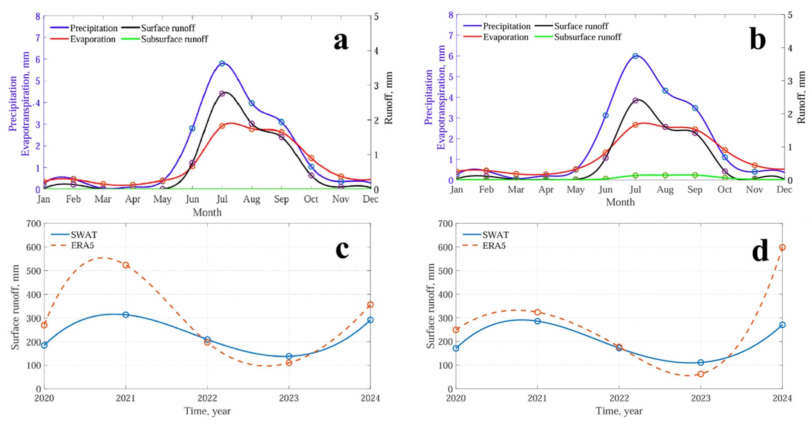
SWAT accurately reproduced the seasonal patterns of the water balance, enabling the quantification of differences in monthly mean flows between the local and regional scales (Figure 4). In Figure 4, values expressed in mm·d⁻¹ correspond to the mean of daily simulations within each month (Figure 4a,b), whereas runoff expressed in mm represents the accumulated monthly total derived from daily simulations (Figure 4c,d). Peak values (mm·d⁻¹) reported in

Table 4. Summary of peak hydrological events and system response dynamics simulated for the Rio Verde Grande Basin and El Niágara Dam.

Parameter	Rio Verde Grande Basin	El Niágara Dam
Peak precipitation (mmd−1)	6	5.8 mm
Peak runoff (mmd−1)	2.4 mm	2.8 mm
Peak evapotranspiration (mmd−1)	2.7 mm	2.9 mm
Max. Lateral flow (Latq) (mmd−1)	0.15	0
Hydrological response	Moderate	Rapid and intense

denote the maximum monthly mean daily values during the analysis period. Spatial scale directly influenced the magnitude of hydrological fluxes, although both domains exhibited a seasonal regime in which runoff was confined to the wet period, when rainfall exceeded evaporative losses (June–September). Table 4 summarizes the maximum mean values of the principal hydrological components for both scales.

At the local scale (El Niágara Dam, Figure 4a), hydrological processes exhibit greater intensity relative to the rainfall input. Peak monthly precipitation averages (5.8 mm·d⁻¹) drive elevated surface runoff (2.8 mm·d⁻¹) and evapotranspiration (2.9 mm·d⁻¹). The system is dominated almost entirely by surface flow; the absence of lateral flow (0 mm·d⁻¹) reflects limited subsurface storage capacity, promoting runoff generation through an immediate Hortonian-type response. This minimal subsurface buffering underlies the classification of the local hydrological behavior as “rapid and intense.”

In contrast, at the regional scale (basin outlet, Figure 4b), hydrological behavior is more moderate. While peak precipitation is slightly higher (6.0 mm·d⁻¹), the resulting surface runoff (2.4 mm·d⁻¹) and evapotranspiration (2.7 mm·d⁻¹) remain lower than those observed locally. Crucially, unlike the El Niágara system, the regional basin exhibits measurable subsurface flow (0.15 mm·d⁻¹). This indicates the presence of basin-level storage processes that are not apparent at finer spatial scales. These subsurface components act as hydrological buffers that dampen runoff peaks, resulting in a distinctly moderated response. In the present configuration, channel transmission losses were not explicitly parameterized (CH_K2 = 0); therefore, the observed attenuation primarily reflects soil moisture storage, lateral flow, and shallow groundwater contributions represented within SWAT+, rather than infiltration losses along channel reaches.

The analysis of interannual variability (Figure 4c,d) shows that SWAT effectively captures the temporal sequence of dry and wet years identified by the ERA5 reanalysis, though notable differences in magnitude emerge. At the local scale (Figure 4c), the model shows reasonable agreement with ERA5 during average years (e.g., 2022–2023), although the reanalysis tends to estimate higher runoff during wet periods. However, a striking divergence is observed at the regional scale (Figure 4d) during the extreme event of 2024. While SWAT simulates a high-flow response consistent with local observations (~270 mm), ERA5 estimates surge to nearly 600 mm (more than double the modeled value). This suggests that the global reanalysis product may drastically overestimate runoff generation across the larger basin during intense storm seasons, likely by failing to account for the transmission losses and infiltration capacity that the calibrated SWAT model successfully captures.

3.3. Quantification of Intensive Agrochemical Management and Nitrogen Loading Regimes

The empirical characterization of management practices, based on surveys administered to 134 local farmers, indicates an agronomic profile dominated by intensive chemical inputs (

Table 5. Agrochemical management practices derived from farmer surveys, including application rate per application, frequency, nutrient/active ingredient concentration, and estimated annual inputs.

Fertilizers	Amount (kg ha−1 per Application)	Application (Year)	N Concentration g kg−1	Total N (kg N ha−1 Year−1 *)
Phosphonitrate	527.8	5.83	330	1015.4
Ammonium phosphate (MAP)	494.6	7.25	110	398.8
Urea	278.7	2.96	460	379.5
Herbicides	Amount (kg ha−1 per Application)	Application (Year)	Active Ingredient g L−1	Total Active Ingredient ** g ha−1 Year−1
Mesotrione	3.20	1.10	480	8.5
Acetochlor	2.80	1.20	900	15.12
Insecticides	Amount (kg ha−1 per Application)	Application (Year)	Active Ingredient g L−1	Total Active Ingredient g ha−1 Year−1
Spinosyns	6.20	3.10	240	22.32
Chlorantraniliprole	3.10	2.20	200	7.0

* Annual nitrogen input was calculated using the fertilizer rate reported in the farmer surveys and the nitrogen concentration of each fertilizer product according to the following equation: $TotalN\left(\mathrm{kg}\mathrm{N}{\mathrm{ha}}^{-1}{\mathrm{year}}^{-1}\right)=amount\left(\mathrm{kg}{\mathrm{ha}}^{-1}\mathrm{per}\mathrm{application}\right)\times applications\left({\mathrm{year}}^{-1}\right)\times \left[Nconcentration{\displaystyle \frac{\left(\mathrm{g}{\mathrm{kg}}^{-1}\right)}{1000}}\right]$. ** Annual active ingredient was calculated using the herbicide and insecticide rates reported in the farmer surveys and the active ingredient concentration of each compound product according to the following equation: $TotalActiveingredient\left(\mathrm{g}{\mathrm{ha}}^{-1}{\mathrm{year}}^{-1}\right)=amount\left(\mathrm{kg}{\mathrm{ha}}^{-1}{\mathrm{L}}^{-1}\mathrm{per}\mathrm{application}\right)\times applications\left({\mathrm{year}}^{-1}\right)\times \left[activeingredient{\displaystyle \frac{\left(\mathrm{g}{\mathrm{L}}^{-1}\right)}{200}}\right].$

). The results show a fractional yet highly frequent fertilization regime, with producers applying fertilizers multiple times per year (mean values of 5.83 applications for phosphonitrate and 7.25 for MAP). This pattern effectively maintains a near-continuous supply of nutrients in the topsoil throughout the cropping cycle. Quantitatively, the system depends on high application rates of external fertilizer inputs, notably phosphonitrate, which registers a total accumulated load of 1015.4 kg·ha⁻¹ year⁻¹, followed by urea (379.5 kg·ha⁻¹ year⁻¹) and monoammonium phosphate (398.8 kg·ha⁻¹ year⁻¹).

3.4. Spatial Distribution of Nitrate Loads and Monitoring Network Design

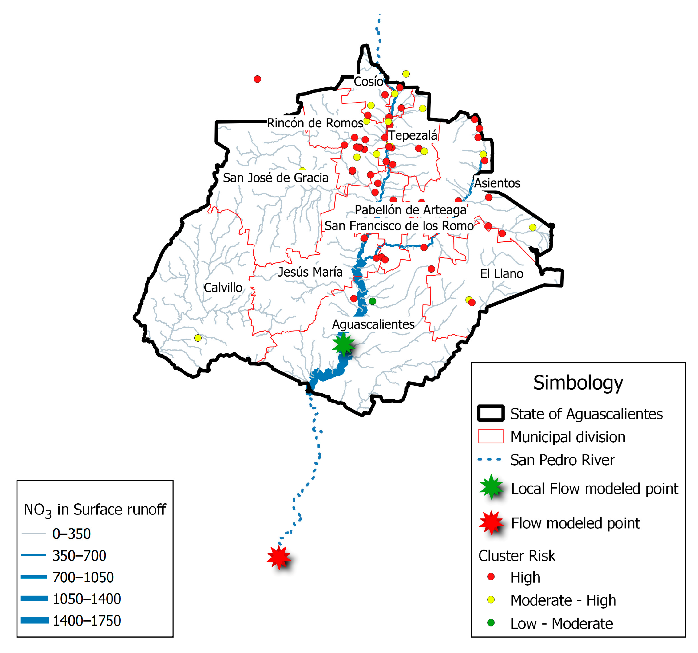
The spatial configuration of nitrate loads (NO₃) in surface runoff (Figure 5) exhibits a distinct north–south gradient. The highest modeled values are concentrated in the northern municipalities of Cosío, Rincón de Romos, Tepezalá, and Pabellón de Arteaga. This hotspot pattern is attributed to the dense clustering of high-risk diffuse sources (red markers), associated with intensive agricultural practices and excessive nitrogen fertilization [2,42]. Furthermore, environmental drivers such as high soil permeability and strong hydrological connectivity to first-order streams are likely to exacerbate these loads in the headwaters [43,44]. Notably, sub-basins classified with higher IRP_N scores spatially coincide with areas exhibiting elevated modeled nitrate accumulation, reinforcing the internal coherence between the survey-derived management risk characterization and the SWAT-simulated hydrological transport patterns.

The spatial configuration of this phenomenon reveals a clear longitudinal accumulation gradient. The highest nitrate loads are transported downstream along the main channel, converging toward the Aguascalientes metropolitan area. This pattern identifies the northern agricultural zone as a critical non-point source area, exporting substantial nutrient loads that compromise water quality in urban receiving systems and increase the regional vulnerability to eutrophication.

To evaluate the propagation of these loads, the monitoring network (Figure 5, stars) was strategically defined at two scales. The Local Flow measurement point (green star) is located at El Niágara Dam, 3 km southwest of Aguascalientes City. This infrastructure was selected as a critical control point because it regulates the hydrological response of the primary agricultural district before the river enters the urban zone. Built in 1959 for flood control and irrigation (supplying 1750 ha on the right bank, including El Salto de los Salado), the dam acts as a sentinel site that integrates the immediate runoff from the high-intensity agricultural HRUs upstream.

In contrast, the Basin Flow measurement point (red star) represents the system’s total output. The longitudinal profile of the San Pedro River (dashed blue line) shows a transition from darker tones in the headwaters to lighter tones downstream, suggesting that the river network provides partial buffering capacity through hydrologic mixing and basin-scale storage processes. Such attenuation patterns are consistent with nitrate transport and transformation dynamics reported in comparable fluvial systems [45,46]. In the present configuration, this attenuation reflects aggregation of upstream contributions and simulated in-stream processes within SWAT+, rather than explicitly parameterized channel transmission losses.

3.5. Temporal Dynamics and Hydrological Response

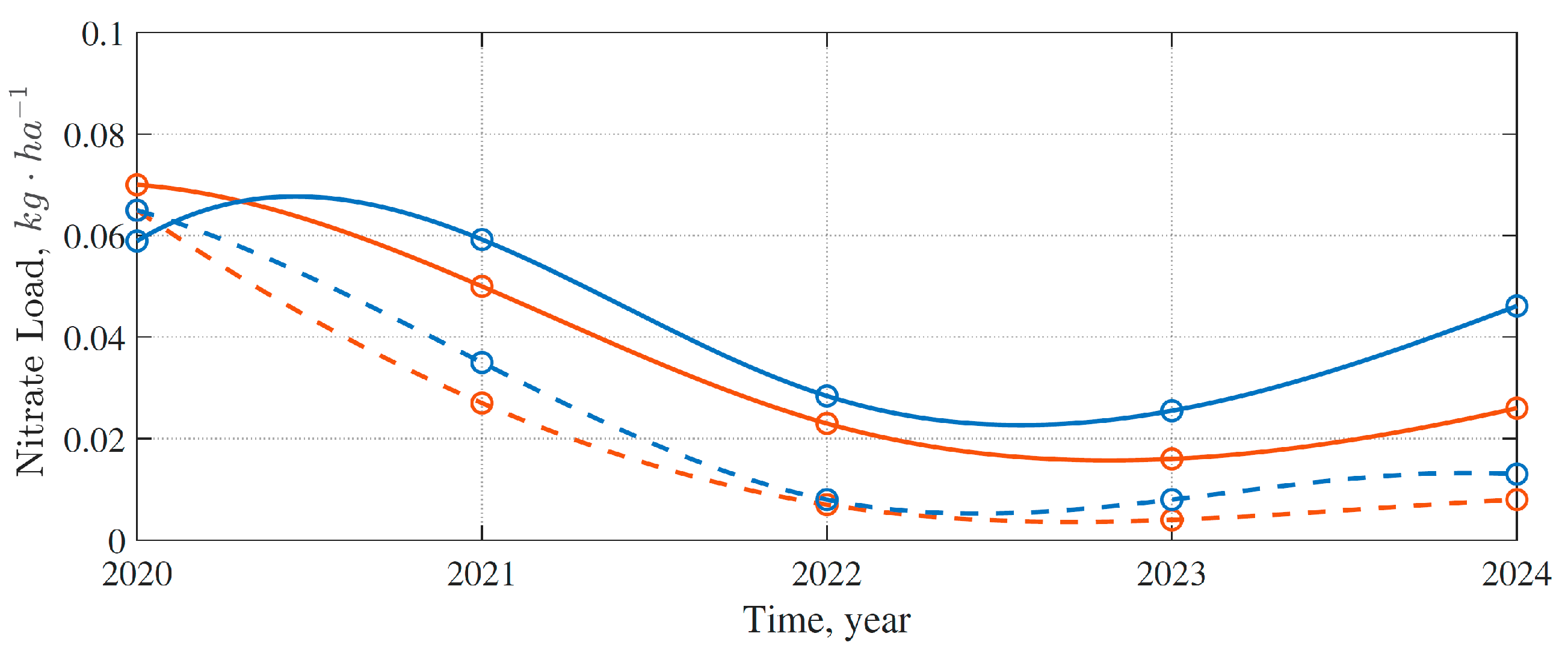
The interaction between the spatial configuration described above and the hydrological regime drives the interannual variability of specific nitrate loads (kg·ha⁻¹), as simulated by SWAT between 2020 and 2024 (Figure 6). The graph allows for a dual comparison between management scenarios (solid vs. dashed lines) and spatial scales (blue vs. red lines).

The analysis highlights the magnitude of anthropogenic forcing. A clear separation is observed where solid lines (active fertilization) exhibit significantly higher nitrate loads compared to the dashed lines (control scenarios). This gap quantifies the direct contribution of agriculture to water quality degradation, confirming that synthetic fertilizers are rapidly mobilized by surface runoff. The simulation captures a “wash-off” mechanism, particularly during the first storm events of the season, where accumulated nutrients are transferred directly into the hydrological network, significantly exceeding the natural baseline capacity of the system.

The hydrological response is strongly modulated by the spatial scale of observation. At the local scale (El Niágara Dam, blue lines), the system exhibits episodic dynamics characterized by abrupt fluctuations. The simulation identifies peak load events reaching ~0.1 kg·ha⁻¹ (notably in 2021), followed by a substantial resurgence in 2024. This behavior arises because the dam’s catchment functions as a direct integrator of specific agricultural Hydrological Response Units (HRUs). In these headwater zones, the combination of intensive land use and steeper slopes enhances hydrological connectivity, consistent with the dominance of surface runoff and limited subsurface contributions at the local scale.

In contrast, the specific load drastically drops at the basin scale (basin outlet, red lines), where values attenuate to lower levels (approximately 0.045 kg·ha⁻¹). The effects of spatial integration are what cause this attenuation. The river receives inflows from a variety of land uses, such as forests and rangelands, which export negligible nitrate loads as the catchment area grows downstream of El Niágara. Consequently, higher concentrations from the agricultural core are gradually diluted by volumes of cleaner runoff. As a result, the basin outlet demonstrates the ability of the river network to partially attenuate upstream inputs through spatial integration and dilution at the basin scale, smoothing the extreme peaks seen at the local scale by representing a weighted average of the entire territory.

The spatial configuration of this phenomenon (Figure 6) indicates a longitudinal accumulation gradient. The highest nitrate loads are transported downstream along the main channel, converging toward the Aguascalientes metropolitan area. This pattern identifies the agricultural zone of the northern Aguascalientes as a critical non-point source area, where prevailing agricultural practices are predominantly classified as high risk (Figure 5), exporting substantial nutrient loads that compromise water quality in urban receiving systems and increase the regional vulnerability to eutrophication.

4. Discussion

4.1. Effect of Forcing Data on Water Balance Simulation

The comparison between SWAT simulations and ERA5 runoff indicates a strong correspondence in seasonal timing and interannual variability, confirming that ERA5 adequately captures the large-scale precipitation dynamics affecting the basin [26,47]. However, during periods of increased runoff magnitude within the analyzed timeframe, particularly in 2024, a marked volumetric divergence emerges between ERA5 runoff and SWAT-simulated runoff. It is important to note that this characterization refers solely to differences in runoff magnitude within the analyzed period (2021–2024), without implying a long-term climatological classification.

Importantly, parameter adjustment was guided primarily by matching temporal variability and seasonal behavior rather than enforcing strict volumetric replication of ERA5 runoff. Therefore, the divergence observed during higher-runoff years reflects differences in runoff magnitude rather than inconsistencies in seasonal timing.

This behavior is consistent with structural differences in spatial resolution and process representation. At a native resolution of ~0.25°, ERA5 represents runoff generation at a coarse regional scale and does not explicitly resolve transmission losses, localized infiltration processes, or channel-aquifer interactions that strongly regulate runoff generation in semi-arid basins [48,49,50,51]. In contrast, the SWAT model incorporates basin-specific soil properties and calibrated hydrological parameters that constrain runoff response under high-intensity rainfall conditions. Consequently, the amplified runoff volumes reflected in the reanalysis product during such periods likely arise from scale-dependent process representation rather than from temporal misrepresentation. The findings presented here should therefore be interpreted within the temporal scope of the analyzed period (2021–2024), acknowledging that longer datasets would allow a more comprehensive evaluation of hydroclimatic variability.

4.2. Sources of Uncertainty and Model Limitations

The results presented in this study are subject to several sources of uncertainty inherent to hydrological and nutrient modeling. Parameter uncertainty arises from the calibration process, particularly for key runoff-related and nitrogen-related parameters, which are known to influence model outputs and nutrient transport dynamics in distributed hydrological models [20,52]. In SWAT applications, uncertainty in parameters such as the curve number and nitrogen transformation coefficients has been shown to contribute substantially to variability in pollutant load estimates, often exceeding uncertainty in simulated streamflow during peak events [53].

Forcing uncertainty is associated with the use of reanalysis or interpolated meteorological inputs. Hydrological models driven by coarse-resolution forcing data may exhibit predictive uncertainty due to the limited representation of localized precipitation variability and hydrometeorological processes, which can affect both water balance and constituent transport simulations [54].

Structural uncertainty stems from simplifications in the model’s conceptual representation of hydrological and biogeochemical processes, including assumptions about subsurface flow pathways and nitrogen cycling. Numerous studies have emphasized that structural choices and input data limitations can lead to systematic differences between simulated and real-world responses, highlighting the importance of explicitly acknowledging structural uncertainty in model interpretation [20,55].

Structural limitations inherent to distributed hydrological models have been widely documented [24,54]. In semi-arid environments, the representation of transmission losses, episodic recharge, and groundwater abstraction remains simplified, potentially affecting long-term nitrate export estimates.

In semi-arid basins characterized by aquifer overexploitation, nitrate transport may also occur through subsurface pathways, including percolation to shallow aquifers and episodic recharge during high-intensity rainfall events. Although SWAT represents shallow groundwater contributions through conceptual reservoirs, it does not explicitly resolve deep aquifer dynamics or complex groundwater-surface water interactions. Therefore, the simulated nitrate loads primarily reflect surface and near-surface transport processes and may underestimate longer-term groundwater contamination risks. This limitation should be considered when interpreting vulnerability patterns in regions where groundwater extraction plays a dominant role in water supply.

Importantly, the present analysis emphasizes relative spatial patterns and hotspot identification rather than precise absolute load quantification. The stability of spatial risk patterns supports the robustness of the proposed framework for comparative and management-oriented purposes within the analyzed period (2021–2024). Nevertheless, future work incorporating formal uncertainty propagation methods, such as Generalized Likelihood Uncertainty Estimation (GLUE) or SUFI-2, would further strengthen quantitative confidence in nitrate load estimates and management-oriented applications.

4.3. Scale-Dependent Hydrological Response

The comparative analysis of the components of the water balance reveals a non-linear relationship between the scale of the watershed and its hydrological response. This is a characteristic phenomenon of semi-arid regions, the intensity of which in this particular area is amplified by land use patterns. The results show a clear spatial transition: from a rapid and intense response at the local scale (El Niágara Dam) to a notably dampened response at the full watershed scale (Outlet).

In the headwaters, the absolute predominance of surface runoff, along with a marginal contribution from lateral flow, indicates a regime dominated by excess infiltration mechanisms (Hortonian). This pattern is typical of small agricultural watersheds with confined topography, where soil compaction resulting from intensive machinery use, a documented fact in local studies, drastically reduces hydraulic conductivity and prevents subsurface saturation [56]. Consequently, precipitation is almost immediately transformed into direct flow, generating a rapid response system with very short concentration times. This interpretation aligns with observations made by Descroix et al. [57] in cultivated headwaters, where sparse vegetation cover and low soil macroporosity accelerate runoff, limiting the activation of slower subsurface flows.

Conversely, at the regional scale, a marked hydrological attenuation is observed. The emergence of measurable subsurface flow and the reduction in specific peak flow at the watershed outlet reflect two key processes: losses due to infiltration in ephemeral channels and the spatial averaging effect of rainfall in extensive watersheds. In semi-arid areas, these channels act as recharge zones, absorbing a significant fraction of the flow as it moves downstream [58]. This process, combined with the activation of alluvial aquifers in the valleys, explains the “natural attenuation” capacity captured by the model. Consequently, hydrological risk is fundamentally scale-dependent: the danger of flash floods is concentrated in the agricultural headwater areas (El Niágara), while the lower part of the watershed benefits from the system’s intrinsic capacity to modulate and delay these water pulses [45].

4.4. Agricultural Drivers and the Potential Nitrate Leaching Risk Index

Due to the limited availability of observed nitrate concentration data for calibration in the study area, we calibrated and validated SWAT using ERA5-derived surface runoff for the study period (2021–2024). The model achieved strong performance metrics during calibration (NSE = 0.87, R² = 0.88, PBIAS = −13.23%, RSR = 0.34) and validation (NSE = 0.76, R² = 0.95), indicating reliable reproduction of runoff dynamics that control nitrate mobilization in semi-arid agricultural watersheds [24,54]. These results support the application of SWAT under conditions where observed nitrate data are unavailable while maintaining acceptable model performance. In addition, we derived fertilizer nitrogen inputs from farmer surveys conducted across the study area, improving the representation of local agricultural management practices. SWAT simulates nitrogen transformations under mass balance principles that constrain nutrient dynamics within the system. We also compared simulated nitrate loads with ranges reported for agricultural watersheds in the literature, providing an additional plausibility check for the modeled results. Therefore, the analysis focuses on relative spatial patterns of nitrate mobilization and hotspot identification rather than on precise absolute load quantification.

The Potential Nitrate Leaching Risk Index (IRP_N) was independently constructed from agronomic and site-specific management variables and subsequently interpreted in relation to the spatial patterns revealed by the unsupervised clustering. The survey results confirm that the “red” clusters identified in the spatial analysis are not random but are characterized by an unsustainable agronomic regime: frequent applications of phosphonitrate and urea that exceed crop uptake capacity. When these high nitrogen inputs (accumulated loads > 1300 kg·ha⁻¹) coincide with a rapid hydrological response simulated by SWAT, the system exhibits conditions consistent with a critical mobilization threshold. The lack of soil retention capacity facilitates the rapid mobilization of nitrates, providing spatially convergent, process-based support for the robustness of the IRP_N in identifying non-point source hotspots. The “wash-off” mechanism implies that in these high-risk zones (Northern Municipalities), the soil acts less like a filter and more like a conveyor belt, transporting agrochemicals directly into the surface water network [46,59,60].

4.5. Social Impact and Policy Implications

The translation of these hydrological and chemical dynamics into a social context reveals a dual vulnerability for the region. First, from an economic perspective, the “wash-off” of nitrates represents a direct financial loss for local farmers. The high application rates detected in the surveys, combined with the rapid runoff response, imply that a significant portion of the purchased fertilizer is lost to the river rather than being assimilated by crops. This inefficiency increases production costs without guaranteeing higher yields. Second, regarding public health and equity, the downstream accumulation of these loads poses a risk to the Aguascalientes Metropolitan Area. Although the river network provides some natural attenuation (dilution from 0.1 to 0.045 kg·ha⁻¹), the transport of dissolved loads from the rural north to the urban center effectively transfers an environmental liability. The eutrophication potential in reservoirs and the risk of aquifer contamination (via infiltration of nitrate-rich runoff) threaten the water security of a growing population. Therefore, the Potential Nitrate Leaching Risk Index should be adopted not just as a scientific metric, but as a policy instrument to target subsidies for “precision agriculture” specifically in the high-risk clusters, simultaneously protecting farmer incomes and public health.

4.6. Management Implications

The spatial differentiation of nitrate risk identified in this study provides a basis for targeted management strategies. High-risk sub-basins may be prioritized for fertilizer optimization programs and nutrient management planning. Clusters classified as high IRP_N risk could inform the strategic placement of groundwater and surface water monitoring stations to improve early detection of contamination. Additionally, areas exhibiting elevated simulated nitrate loads under fertilized scenarios may represent suitable locations for pilot precision-agriculture initiatives aimed at reducing input intensity while maintaining productivity. These targeted actions enhance the operational value of the proposed framework for integrated water and nutrient management in semi-arid regions.

Beyond the present case study, the proposed framework is transferable to other semi-arid basins where process-based hydrological modeling can be combined with management-oriented datasets. Its implementation, however, requires (i) spatially consistent watershed configuration data, (ii) reliable hydro-climatic forcing, and (iii) structured agricultural survey information capturing fertilizer practices. In regions lacking detailed management data, the IRP_N component would require adaptation to locally available indicators. Thus, while methodological architecture can be generalized, its operational application remains context-dependent and sensitive to data availability and quality.

5. Conclusions

This study characterizes the hydrology of the headwaters of the Aguascalientes River, revealing that the system is subject to significant anthropogenic pressure. The results indicate that the SWAT model is capable of reproducing the watershed’s hydrological signals. However, the use of global ERA5 data is not a ready-to-use solution for this type of semi-arid basin: although it accurately captures the synoptic timing of precipitation, it tends to overestimate discharge volumes. Therefore, reanalysis data cannot replace local gauging without rigorous bias correction.

The basin’s dynamics are governed by a pronounced scale-dependent duality. The headwaters operate as a surface-dominated system characterized by a Hortonian runoff regime, in which agricultural soil compaction has effectively sealed the subsoil. This agronomic imprint suppresses natural retention processes, forcing rainfall to bypass infiltration pathways and converting headwater channels into high-velocity flow conduits. In contrast, the lower basin exhibits a greater attenuation capacity at the basin scale, where spatial integration and distributed soil and shallow groundwater storage processes dampen the flood pulse. This fundamental result demonstrates that flood hazards are not spatially uniform but are generated upstream and mitigated downstream through basin-scale hydrological aggregation.

Concerning water quality, the IRP_N serves as a diagnostic tool for agronomic inefficiency. The identification of risk groups correlates directly with fertilization rates that defy physiological logic (>1000 kg N·ha⁻¹ year⁻¹) by exceeding the crop’s absorption capacity. This creates a scenario of “chemical saturation,” where excess nitrogen (unabsorbed by the crop) is mobilized by rapid runoff, acting as a fast transport vector that delivers dissolved nutrients directly to the river network before the soil can process them.

These findings indicate that improving water security in the basin depends less on additional infrastructure and more on optimized soil and nutrient management. Adopting precision agriculture and soil restoration practices would reduce nutrient losses, enhance hydrological function, and bolster both environmental and economic sustainability.

References

1. INEGI. Aspectos Geográficos de Aguascalientes: Compendio 2022; Instituto Nacional de Estadística, Geografía e Informática: Aguascalientes, Mexico, 2022. [Google Scholar]
2. Biswas, A.; Sarkar, S.; Das, S.; Dutta, S.; Roy Choudhury, M.; Giri, A.; Bera, B.; Bag, K.; Mukherjee, B.; Banerjee, K.; et al. Water scarcity: A global hindrance to sustainable development and agricultural production–A critical review of the impacts and adaptation strategies. Camb. Prism. Water 2025, 3, e4. [Google Scholar] [CrossRef] [Scilit]
3. McDonald, R.I.; Green, P.; Balk, D.; Fekete, B.M.; Revenga, C.; Todd, M.; Montgomery, M. Urban growth, climate change, and freshwater availability. Proc. Natl. Acad. Sci. USA 2011, 108, 6312–6317. [Google Scholar] [CrossRef] [Scilit]
4. Gutiérrez-Ojeda, C.; Escolero-Fuentes, O.A. Groundwater Resources of Mexico. In Water Resources of Mexico; Raynal-Villasenor, J.A., Ed.; Springer International Publishing: Cham, Switzerland, 2020; pp. 15–33. [Google Scholar]
5. CONAGUA. Atlas del Agua en México; Secretaría de Medio Ambiente y Recursos Naturales: Ciudad de México, Mexico, 2023. [Google Scholar]
6. Liu, M.; Zhou, X.; Huang, G.; Li, Y. The increasing water stress projected for China could shift the agriculture and manufacturing industry geographically. Commun. Earth Environ. 2024, 5, 396. [Google Scholar] [CrossRef] [Scilit]
7. Novoa, V.; Rojas, C.; Rojas, O.; Ahumada-Rudolph, R.; Moreno-Santoyo, R. A temporal analysis of the consequences of the drought regime on the water footprint of agriculture in the Guadalupe Valley, Mexico. Sci. Rep. 2024, 14, 6114. [Google Scholar] [CrossRef] [Scilit]
8. Pacheco-Treviño, S.; Manzano-Camarillo, M.G.F. Review of water scarcity assessments: Highlights of Mexico’s water situation. Wiley Interdiscip. Rev. Water 2024, 11, e1721. [Google Scholar] [CrossRef] [Scilit]
9. Scanlon, B.R.; Fakhreddine, S.; Rateb, A.; de Graaf, I.; Famiglietti, J.; Gleeson, T.; Grafton, R.Q.; Jobbagy, E.; Kebede, S.; Kolusu, S.R.; et al. Global water resources and the role of groundwater in a resilient water future. Nat. Rev. Earth Environ. 2023, 4, 87–101. [Google Scholar] [CrossRef] [Scilit]
10. Zhang, C.; Xiao, X.; Wang, X.; Yi, S.; Meng, C.; Qin, Y.; Yao, Y.; Yin, L.; Celis, J.; Pan, L.; et al. Climate-induced losses of surface water and total water storage in Northeast Asia. Commun. Earth Environ. 2025, 6, 479. [Google Scholar] [CrossRef] [Scilit]
11. Liu, X.; Yang, L.; Liu, L.; Fu, W.; Wu, C. SWAT-Based Characterization of Agricultural Area-Source Pollution in a Small Basin. Water 2025, 17, 388. [Google Scholar] [CrossRef] [Scilit]
12. Bekić, D.; Leskovar, K. Evaluating CHIRPS and ERA5 for Long-Term Runoff Modelling with SWAT in Alpine Headwaters. Water 2025, 17, 2116. [Google Scholar] [CrossRef] [Scilit]
13. Comisión Nacional del Agua. Estadísticas del Agua en México, Edición 2018; Secretaría de Medio Ambiente y Recursos Naturales: Ciudad de México, Mexico, 2018. [Google Scholar]
14. Beharry, S.L.; Gabriels, D.; Lobo, D.; Ramsewak, D.; Clarke, R.M. Use of the SWAT model for estimating reservoir volume in the Upper Navet watershed in Trinidad. SN Appl. Sci. 2021, 3, 163. [Google Scholar] [CrossRef] [Scilit]
15. Cruz-González, A.; Sánchez-Cohen, I.; Macías-Corral, M.A.; Velásquez-Valle, M.A.; Trejo-Calzada, R. Hydrologic modeling to measure the impact of climate change in the Yaqui River basin. Ing. Agrícola Biosist. 2021, 13, 77–94. [Google Scholar] [CrossRef] [Scilit]
16. Moriasi, D.N.; Arnold, J.G.; Van Liew, M.W.; Bingner, R.; Harmel, R.D.; Veith, T.L. Model Evaluation Guidelines for Systematic Quantification of Accuracy in Watershed Simulations. Trans. ASABE 2007, 50, 885–900. [Google Scholar] [CrossRef] [Scilit]
17. Abbaspour, K.C. SWAT Calibration and Uncertainty Programs–A User Manual; Swiss Federal Institute of Aquatic Science and Technology: Dübendorf, Switzerland, 2015; p. 100. [Google Scholar]
18. Nash, J.E.; Sutcliffe, J.V. River flow forecasting through conceptual models part I—A discussion of principles. J. Hydrol. 1970, 10, 282–290. [Google Scholar] [CrossRef] [Scilit]
19. Gupta, H.V.; Sorooshian, S.; Yapo, P.O. Status of Automatic Calibration for Hydrologic Models: Comparison with Multilevel Expert Calibration. J. Hydrol. Eng. 1999, 4, 135–143. [Google Scholar] [CrossRef] [Scilit]
20. Abbaspour, K.C.; Rouholahnejad, E.; Vaghefi, S.; Srinivasan, R.; Yang, H.; Kløve, B. A continental-scale hydrology and water quality model for Europe: Calibration and uncertainty of a high-resolution large-scale SWAT model. J. Hydrol. 2015, 524, 733–752. [Google Scholar] [CrossRef] [Scilit]
21. Comisión Nacional para el Conocimiento y Uso de la Biodiversidad (CONABIO). Mapa de Uso de Suelo y Vegetación, Serie VI (escala 1:250,000); Map; CONABIO: Ciudad de México, Mexico, 2023. [Google Scholar]
22. INEGI. Modelo Digital de Elevación de México (Continuo de Elevaciones Mexicano 3.0); Mapa digital; INEGI: Ciudad de México, Mexico, 2024. [Google Scholar]
23. Arnold, J.G.; Srinivasan, R.; Muttiah, R.S.; Williams, J.R. Large Area Hydrologic Modeling and Assessment Part I: Model Development. JAWRA J. Am. Water Resour. Assoc. 1998, 34, 73–89. [Google Scholar] [CrossRef] [Scilit]
24. Gassman, P.W.; Reyes, M.R.; Green, C.H.; Arnold, J.G. The Soil and Water Assessment Tool: Historical Development, Applications, and Future Research Directions. Trans. ASABE 2007, 50, 1211–1250. [Google Scholar] [CrossRef] [Scilit]
25. Saha, P.P.; Zeleke, K.; Hafeez, M. Streamflow modeling in a fluctuant climate using SWAT: Yass River catchment in south eastern Australia. Environ. Earth Sci. 2014, 71, 5241–5254. [Google Scholar] [CrossRef] [Scilit]
26. Hersbach, H.; Bell, B.; Berrisford, P.; Hirahara, S.; Horányi, A.; Muñoz-Sabater, J.; Nicolas, J.; Peubey, C.; Radu, R.; Schepers, D.; et al. The ERA5 global reanalysis. Q. J. R. Meteorol. Soc. 2020, 146, 1999–2049. [Google Scholar] [CrossRef] [Scilit]
27. Wilcox, R.R. Introduction to Robust Estimation and Hypothesis Testing, 3rd ed.; Academic Press: San Diego, CA, USA, 2012. [Google Scholar]
28. Correa-González, A.; Hernández-Bedolla, J.; Martínez-Cinco, M.A.; Sánchez-Quispe, S.T.; Hernández-Hernández, M.A. Assessment of Nitrate in Groundwater from Diffuse Sources Considering Spatiotemporal Patterns of Hydrological Systems Using a Coupled SWAT/MODFLOW/MT3DMS Model. Hydrology 2023, 10, 209. [Google Scholar] [CrossRef] [Scilit]
29. Santillano-Cázares, J.; Turmel, M.-S.; Cárdenas-Castañeda, M.E.; Mendoza-Pérez, S.; Limón-Ortega, A.; Paredes-Melesio, R.; Guerra-Zitlalapa, L.; Ortiz-Monasterio, I. Can Biofertilizers Reduce Synthetic Fertilizer Application Rates in Cereal Production in Mexico? Agronomy 2022, 12, 80. [Google Scholar] [CrossRef] [Scilit]
30. R Core Team. R: A Language and Environment for Statistical Computing; R Foundation for Statistical Computing: Vienna, Austria, 2013; Available online: https://www.r-project.org/ (accessed on 24 March 2026).
31. Cambon, J.; Hernangómez, D.; Belanger, C.; Possenriede, D. tidygeocoder: An R package for geocoding. J. Open Source Softw. 2021, 6, 3544. [Google Scholar] [CrossRef] [Scilit]
32. Zhang, Q.; Qian, H.; Xu, P.; Li, W.; Feng, W.; Liu, R. Effect of hydrogeological conditions on groundwater nitrate pollution and human health risk assessment of nitrate in Jiaokou Irrigation District. J. Clean. Prod. 2021, 298, 126783. [Google Scholar] [CrossRef] [Scilit]
33. Jehanzaib, M.; Ajmal, M.; Achite, M.; Kim, T.-W. Comprehensive Review: Advancements in Rainfall-Runoff Modelling for Flood Mitigation. Climate 2022, 10, 147. [Google Scholar] [CrossRef] [Scilit]
34. Fageria, N.K. The Use of Nutrients in Crop Plants; CRC Press: Boca Raton, FL, USA, 2016. [Google Scholar] [CrossRef] [Scilit]
35. Serra, J.; Cameira, M.d.R.; Cordovil, C.M.d.S.; Hutchings, N.J. Development of a groundwater contamination index based on the agricultural hazard and aquifer vulnerability: Application to Portugal. Sci. Total Environ. 2021, 772, 145032. [Google Scholar] [CrossRef] [Scilit]
36. Adzawla, W.; Setsoafia, E.D.; Setsoafia, E.D.; Amoabeng-Nimako, S.; Atakora, W.K.; Bindraban, P.D. Accuracy of agricultural data and implications for policy: Evidence from maize farmer recall surveys and crop cuts in the Guinea Savannah zone of Ghana. Agric. Syst. 2024, 214, 103817. [Google Scholar] [CrossRef] [Scilit]
37. LaFevor, M.C. Characterizing Agricultural Diversity with Policy-Relevant Farm Typologies in Mexico. Agriculture 2022, 12, 1315. [Google Scholar] [CrossRef] [Scilit]
38. Nardo, M.; Saisana, M.; Saltelli, A.; Tarantola, S.; Hoffman, A.; Giovannini, E. Handbook on Constructing Composite Indicators: Methodology and User Guide; OECD Publishing: Paris, France, 2005. [Google Scholar]
39. Husson, F.; Lê, S.; Pagès, J. Exploratory Multivariate Analysis by Example Using R, 2nd ed.; CRC Press: Boca Raton, FL, USA, 2017; Volume 15. [Google Scholar]
40. Greenacre, M.; Blasius, J. Multiple Correspondence Analysis and Related Methods, 1st ed.; Chapman and Hall/CRC: Boca Raton, FL, USA, 2006. [Google Scholar]
41. Lezhnina, O.; Kismihók, G. Latent Class Cluster Analysis: Selecting the number of clusters. MethodsX 2022, 9, 101747. [Google Scholar] [CrossRef] [Scilit]
42. Mekonnen, M.M.; Hoekstra, A.Y. Four billion people facing severe water scarcity. Sci. Adv. 2016, 2, e1500323. [Google Scholar] [CrossRef] [Scilit]
43. Song, J.-H.; Her, Y.; Guo, T. Quantifying the contribution of direct runoff and baseflow to nitrogen loading in the Western Lake Erie Basins. Sci. Rep. 2022, 12, 9216. [Google Scholar] [CrossRef] [Scilit] [PubMed]
44. Wang, Y.; Lin, J.; Wang, F.; Tian, Q.; Zheng, Y.; Chen, N. Hydrological connectivity affects nitrogen migration and retention in the land–river continuum. J. Environ. Manag. 2023, 326, 116816. [Google Scholar] [CrossRef] [Scilit]
45. Blöschl, G.; Sivapalan, M. Scale issues in hydrological modelling: A review. Hydrol. Process. 1995, 9, 251–290. [Google Scholar] [CrossRef] [Scilit]
46. Bieroza, M.Z.; Heathwaite, A.L.; Mullinger, N.J.; Keenan, P.O. Understanding nutrient biogeochemistry in agricultural catchments: The challenge of appropriate monitoring frequencies. Environ. Sci. Process. Impacts 2014, 16, 1676–1691. [Google Scholar] [CrossRef] [Scilit]
47. Tarek, M.; Brissette, F.P.; Arsenault, R. Evaluation of the ERA5 reanalysis as a potential reference dataset for hydrological modelling over North America. Hydrol. Earth Syst. Sci. 2020, 24, 2527–2544. [Google Scholar] [CrossRef] [Scilit]
48. Nogueira, M. Inter-comparison of ERA-5, ERA-interim and GPCP rainfall over the last 40 years: Process-based analysis of systematic and random differences. J. Hydrol. 2020, 583, 124632. [Google Scholar] [CrossRef] [Scilit]
49. Xiang, Y.; Chen, J.; Li, L.; Peng, T.; Yin, Z. Evaluation of Eight Global Precipitation Datasets in Hydrological Modeling. Remote Sens. 2021, 13, 2831. [Google Scholar] [CrossRef] [Scilit]
50. Essou, G.R.C.; Arsenault, R.; Brissette, F.P. Comparison of climate datasets for lumped hydrological modeling over the continental United States. J. Hydrol. 2016, 537, 334–345. [Google Scholar] [CrossRef] [Scilit]
51. Beck, H.E.; Vergopolan, N.; Pan, M.; Levizzani, V.; van Dijk, A.I.J.M.; Weedon, G.P.; Brocca, L.; Pappenberger, F.; Huffman, G.J.; Wood, E.F. Global-scale evaluation of 22 precipitation datasets using gauge observations and hydrological modeling. Hydrol. Earth Syst. Sci. 2017, 21, 6201–6217. [Google Scholar] [CrossRef] [Scilit]
52. Shrestha, S.; Shrestha, M.; Shrestha, P.K. Evaluation of the SWAT model performance for simulating river discharge in the Himalayan and tropical basins of Asia. Hydrol. Res. 2017, 49, 846–860. [Google Scholar] [CrossRef] [Scilit]
53. Wu, Y.; Liu, S. Automating calibration, sensitivity and uncertainty analysis of complex models using the R package Flexible Modeling Environment (FME): SWAT as an example. Environ. Model. Softw. 2012, 31, 99–109. [Google Scholar] [CrossRef] [Scilit]
54. Arnold, J.G.; Moriasi, D.N.; Gassman, P.W.; Abbaspour, K.C.; White, M.J.; Srinivasan, R.; Santhi, C.; Harmel, R.D.; van Griensven, A.; Van Liew, M.W.; et al. SWAT: Model Use, Calibration, and Validation. Trans. ASABE 2012, 55, 1491–1508. [Google Scholar] [CrossRef] [Scilit]
55. Beven, K.; Binley, A. The future of distributed models: Model calibration and uncertainty prediction. Hydrol. Process. 1992, 6, 279–298. [Google Scholar] [CrossRef] [Scilit]
56. García-Ruiz, J.M. The effects of land uses on soil erosion in Spain: A review. Catena 2010, 81, 1–11. [Google Scholar] [CrossRef] [Scilit]
57. Descroix, L.; Viramontes, D.; Estrada, J.; Gonzalez Barrios, J.-L.; Asseline, J. Investigating the spatial and temporal boundaries of Hortonian and Hewlettian runoff in Northern Mexico. J. Hydrol. 2007, 346, 144–158. [Google Scholar] [CrossRef] [Scilit]
58. Goodrich, D.C.; Lane, L.J.; Shillito, R.M.; Miller, S.N.; Syed, K.H.; Woolhiser, D.A. Linearity of basin response as a function of scale in a semiarid watershed. Water Resour. Res. 1997, 33, 2951–2965. [Google Scholar] [CrossRef] [Scilit]
59. Scanlon, B.R.; Reedy, R.C.; Stonestrom, D.A.; Prudic, D.E.; Dennehy, K.F. Impact of land use and land cover change on groundwater recharge and quality in the southwestern US. Glob. Change Biol. 2005, 11, 1577–1593. [Google Scholar] [CrossRef] [Scilit]
60. Dupas, R.; Gascuel-Odoux, C.; Gilliet, N.; Grimaldi, C.; Gruau, G. Distinct export dynamics for dissolved and particulate phosphorus reveal independent transport mechanisms in an arable headwater catchment. Hydrol. Process. 2015, 29, 3162–3178. [Google Scholar] [CrossRef] [Scilit]
Figure 1. Geographic location of the study area. (a) Location of the state of Aguascalientes (black outline) within the Lerma–Santiago Hydrological Region VIII (ochre) in Mexico, including the main channel of the San Pedro River (blue line). (b) Modeled domain corresponding to the Río Verde Grande basin, showing the official sub-basins (polygons numbered 1–12). The Upper Aguascalientes watershed corresponds to sub-basin 7 within this basin, where the San Pedro River forms the main channel. The state boundary (thick black outline) and adjacent state divisions (gray lines) are shown. Yellow dots indicate the locations of the 134 agricultural producer surveys. The red star indicates the modeled basin outlet point, and the red circle indicates the nearest ERA5 grid cell used as the surface runoff reference for parameter adjustment. The green star indicates the local modeled point at Niagara (see text), and the green circle indicates the corresponding ERA5 reference point. Black dots indicate the ERA5 grid points used as meteorological inputs to SWAT.
Hydrology 13 00105 g001
Figure 2. Biophysical characteristics of the study basin. (a) Land use and vegetation cover map [21]. (b) Digital Elevation Model [22]. The black outline in both panels delineates the state boundary of Aguascalientes.
Hydrology 13 00105 g002
Figure 3. Integrated methodological workflow for nitrate vulnerability assessment. The framework illustrates the parallel development of (left) SWAT-based hydrological modeling under two management scenarios and (right) the survey-derived Composite Risk Index (IRPN). Integration of both components occurs during the spatial comparison and interpretation phase.
Hydrology 13 00105 g003
Figure 4. Monthly hydrological balance simulated with SWAT for (a) El Niágara Dam and (b) the Río Verde Grande basin, showing precipitation (blue), evapotranspiration (red), surface runoff (black), and subsurface runoff (green). Annual surface runoff time series for (c) El Niágara Dam and (d) the basin outlet, comparing the SWAT simulation (solid blue line) with ERA5 reanalysis estimates (dashed red line).
Hydrology 13 00105 g004
Figure 5. Spatial distribution of specific nitrate (NO3) loads in surface runoff and their longitudinal accumulation along the main river network. The San Pedro River is shown in blue dashed line, municipal boundaries in red, and colored dots indicate cluster-based risk categories (red: High; yellow: Moderate–High; green: Low–Moderate). The stars mark the flow measurement stations: green for the local point (El Niágara Dam) and red for the basin outlet.
Hydrology 13 00105 g005
Figure 6. Interannual variability of specific nitrate loads (kg·ha−1) simulated by SWAT (2020–2024). The graph compares management scenarios and spatial scales: solid lines represent active fertilization, while dashed lines indicate control scenarios. Blue lines correspond to the local modeled point at El Niágara Dam (reflecting direct agricultural response), and orange lines represent the integrated response at the basin outlet.
Hydrology 13 00105 g006