
Article

Hydrological Model Calibration in Data-Scarce Mediterranean Catchments: A Comparative Assessment of Three Strategies

1
Department of Civil, Architectural and Environmental Engineering, University of Naples Federico II, 80125 Naples, Italy
2
University School of Advanced Studies IUSS Pavia, 27100 Pavia, Italy
3
Consorzio Interuniversitario per l’Idrologia (CINID), 85100 Potenza, Italy
4
Autorità di Bacino Distrettuale dell’Appennino Meridionale, 81100 Caserta, Italy
*
Author to whom correspondence should be addressed.
Hydrology 2026, 13(2), 66; https://doi.org/10.3390/hydrology13020066
Submission received: 11 December 2025 / Revised: 14 January 2026 / Accepted: 1 February 2026 / Published: 9 February 2026

Abstract

Hydrological calibration in data-scarce catchments is challenged by non-stationary regimes, fragmented data, and systematic measurement errors. Conventional calibration approaches often assume continuous records and rely on standard performance metrics, which can bias calibration toward high flows and exacerbate parameter equifinality—ultimately reducing robustness under data limitations. This study provides a systematic comparison of three calibration strategies—Kling–Gupta Efficiency (KGE), a non-parametric variant (RNP), and Flow Duration Curve (FDC)-based calibration—together with their time-consistent counterparts (SKGE, SRNP, and SRMSE). All schemes are implemented for the lumped HBV-type TUW model across nine catchments in southern Italy and evaluated using independent metrics targeting overall hydrograph agreement, high-flow behavior, and FDC quantile matching (Q5–Q95). The results reveal that the time-consistent KGE-based strategy excels during in calibration (NSE = 0.56, RMSE = 4.65 m3/s) but shows notable declines in validation (NSE = 0.40, RMSE = 3.91 m3/s), indicating sensitivity to non-stationarity. The RNP-based approach demonstrates enhanced validation robustness (NSE = 0.51, RMSE = 3.60 m3/s) and low-flow accuracy, with NSElnQ = 0.30 and low-flow accuracy, leveraging its non-parametric structure. The SRNP variant further enhances performance in validation (NSE = 0.52, RMSE = 3.42 m3/s), along with superior low-flow performance (NSElnQ = 0.48). The FDC-based strategy effectively reproduces flow distributions during calibration (NSE = 0.41, minimal PBIAS = −0.03%) but exhibits limited temporal transferability (validation NSE = 0.25, RMSE = 4.50 m3/s). Time-consistent variants reduce parameter dispersion by approximately 2–8% (relative to full-period calibration) and improve validation metrics by 5–15% across all catchments. Overall, time-consistent calibration provides a practical pathway to increase robustness under non-stationary, data-scarce Mediterranean conditions, highlighting a systematic trade-off between calibration accuracy and validation reliability.

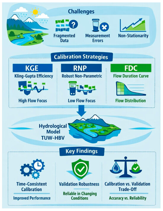
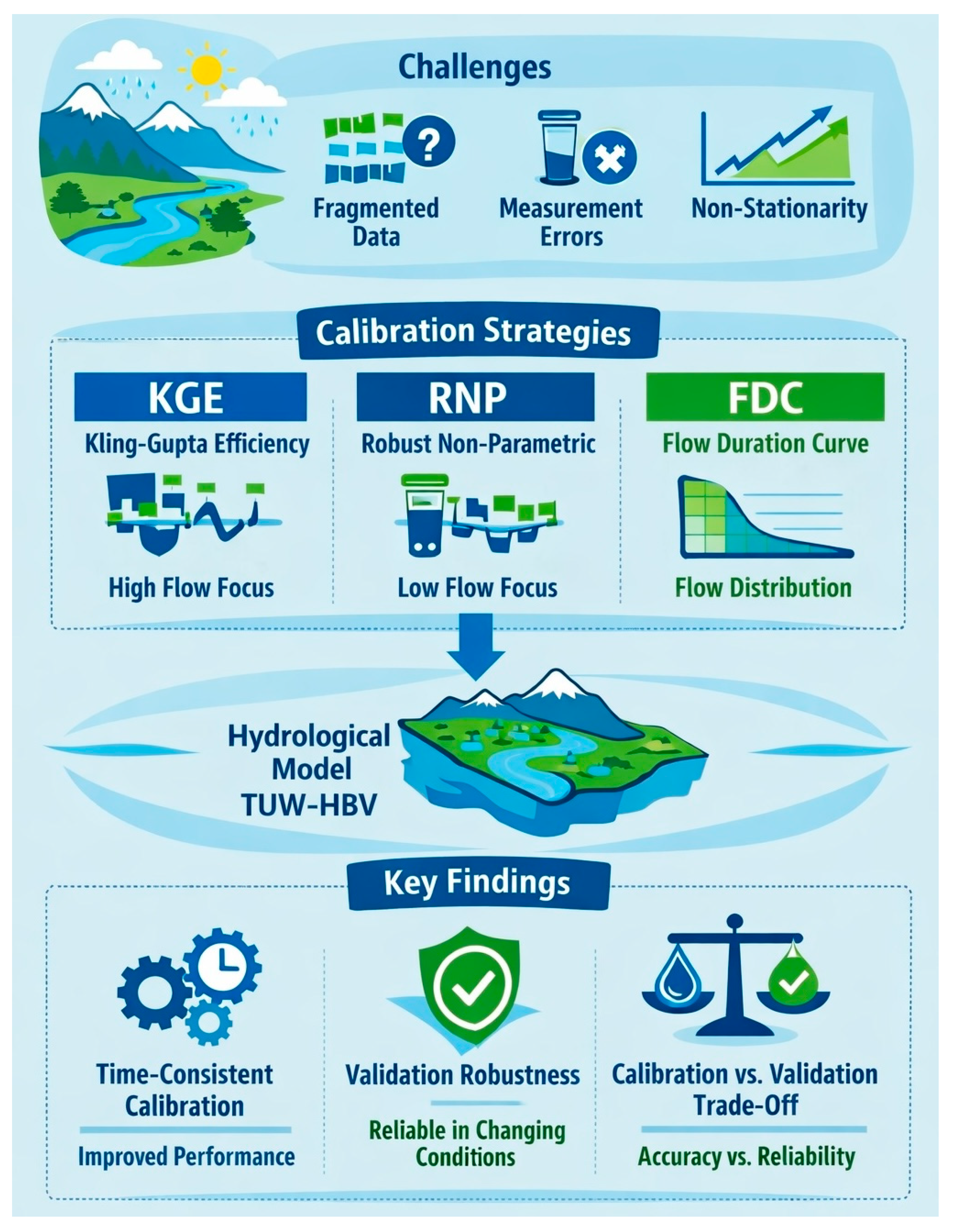
Graphical Abstract

1. Introduction

Hydrological modeling is a cornerstone of effective water resource management, enabling informed decisions in flood risk assessment, drought mitigation, and climate adaptation across diverse global regions [1,2]. Conceptual models balance physical realism with computational efficiency, making them widely adopted for operational and research applications [3]. However, their efficacy hinges on robust calibration, particularly in regions confronting escalating climate variability, anthropogenic influences, and pervasive data scarcity, where traditional approaches often falter [4,5,6].
In data-scarce environments, calibrating conceptual models to align simulations with sparse or discontinuous streamflow observations presents formidable challenges [7,8,9]. Conventional methods, which optimize parameters against daily discharge records using aggregate metrics like the Nash–Sutcliffe Efficiency (NSE) or Kling–Gupta Efficiency (KGE), are beset by several critical shortcomings [10,11]. Primarily, they are highly sensitive to discharge data errors, often exceeding 20–30% [12]. Secondly, global metrics such as NSE prioritize high-flow events, neglecting critical low-flow processes [13,14]. Thirdly, systematic errors in input data, such as rainfall biases, violate statistical likelihood assumptions [15,16]. Compounding these issues are parameter uncertainty and interannual variability that erode calibration stability, especially under non-stationary conditions where historical records fail to encapsulate evolving hydroclimatic regimes, leading to unreliable extrapolations [17].
Emerging literature advocates for refined calibration paradigms to mitigate these deficiencies [18]. Least-squares-based metrics like NSE and KGE frequently yield parameter ensembles that prove brittle under climatic shifts, even when more resilient alternatives exist within the feasible parameter space [19]. Such metrics inherently bias toward peak flows [20,21], heightening vulnerability to rating-curve errors during extremes [22] and overlooking trade-offs across the full flow spectrum [23]. Prioritizing mid- to low-flow calibration or leveraging drier sub-periods as proxies for projected aridification offers a pathway to more pertinent process insights [24]. Hydrological signatures—scalar diagnostics of catchment behavior—provide an alternative lens for performance evaluation, distilling multifaceted dynamics into interpretable indicators [25]. However, signature-based criteria are not immune to equifinality, as their dimensionality reduction can mask structural ambiguities, a limitation that endures even with advanced formulations [13,26].
To surmount these hurdles and foster holistic assessment across flow regimes, multi-metric frameworks have gained traction, integrating hydrograph fidelity, event-specific accuracy, and distributional signatures to offset single-objective biases [21,27]. This multifaceted evaluation is especially relevant to data-scarce settings, where pronounced flow intermittency and regime shifts demand resilient validation protocols [8]. These imperatives are acutely pronounced in Mediterranean basins, such as those in southern Italy, where non-stationary hydrographs—driven by bimodal precipitation, karstic geology, and intensifying human interventions—exacerbate modeling uncertainties [28,29,30].
Signature-based calibration, exemplified by Flow Duration Curve (FDC) matching, has emerged as a potent countermeasure to data sparsity in hydrological modeling [31,32]. By emphasizing empirical flow distributions over temporal sequencing, FDCs circumvent gaps in episodic records and attenuate timing mismatches, proving superior for ephemeral and intermittent regimes [32,33,34,35,36]. Empirical applications underscore their value: Ref. [37] harnessed runoff and soil moisture signatures to curtail parameter uncertainty in 20 Czech catchments via the Bilan model; Ref. [38] augmented metrics for 141 flash-flood-prone Mediterranean basins using signature-sensitivity analyses; and Ref. [39] pioneered Approximate Bayesian Computation (ABC) for FDC and baseflow index assimilation. Similarly, Ref. [40] validated signature-domain methods within the SUPERFLEX framework, deploying HyMod and reservoir configurations to delineate dominant processes. Recent extensions in data-scarce Mediterranean contexts further affirm this trajectory, with hybrid remote sensing integrations enhancing evapotranspiration inputs for improved runoff simulations [41] and multi-conceptual ensembles bolstering streamflow fidelity in ungauged watersheds [42].
Complementing signatures, time-consistent calibration-aggregating objective functions over sub-annual periods tackle interannual non-stationarity and equifinality by enforcing parameter invariance across hydrologic states, thereby curbing overfitting to transient conditions [23]. This strategy attenuates the “divide-and-measure nonconformity” (DAMN) artifact, wherein partition-induced variance shifts distort metrics like NSE [43]. The split KGE (SKGE), for instance, averages KGE over water years to yield temporally nuanced diagnostics, bolstering transferability and process hypothesis testing [44,45]. Integrating these with multi-metric suites yields comprehensive diagnostics, transcending the constraints of monolithic objectives.
Notwithstanding these advances, theoretical critiques of conventional calibration underscore the imperative for empirical inter-comparisons [46,47]. Multi-criteria and acceptability-based frameworks [48] mitigate biases by probing disparate behaviors, yet they presuppose continuous, high-fidelity records and remain susceptible to forcing uncertainties, such as rainfall deficits in ungauged terrains [12,49]. Signature-centric alternatives, while resilient to temporal artifacts, warrant scrutiny in non-stationary Mediterranean settings, where FDC efficacy versus hydrograph-oriented metrics (e.g., KGE) remains underexplored amid regulation and scarcity [39,40,50].
Southern Italy epitomizes these Mediterranean modeling conundrums: its basins, spanning the Apennines to lower catchments, feature intricate hydrology, stark seasonal precipitation contrasts, and dwindling gauge networks—exacerbated by a 50% global drop in streamflow stations since the 1970s [51]. Catchments here rely on fragmented or reconstructed records, compounded by mismatches between local observations and reanalysis products like ERA5 or CHIRPS [52]. Building on antecedent works—such as the DREAM model’s runoff simulation [33,53,54] and physics-informed calibration in the Aniene basin via snow and recession signatures [2]—this study pioneers a rigorous inter-comparison of calibration paradigms tailored to such exigencies.
In essence, calibrating hydrological models in data-scarce Mediterranean catchments is impeded by non-stationary hydrological regimes, monitoring deficits, and epistemic errors. Furthermore, common evaluation paradigms like NSE and KGE are prone to high-flow skew, equifinality, and validation fragility. This lacuna in comparative testing, exacerbated by increasing interannual volatility and hydroclimatic change, demands more streamlined and adaptive strategies for dependable simulations. To address this, our study systematically compares three calibration strategies—implemented through six distinct schemes—for the HBV-based TUW model across nine catchments in southern Italy (five regulated and four natural catchments). Optimizing 15 parameters against tailored objectives, we scrutinize efficacy via six aggregate metrics and five FDC quantiles (Q5–Q95). Our principal aim is to discern optimal strategies for delineating flow dynamics, thereby fortifying water management resilience in these imperiled domains. This analysis not only elucidates trade-offs in calibration fidelity versus generalization but also extends regional modeling precedents by quantifying time-consistency’s role in parameter stability and non-stationary robustness.
Complementing signatures, our time-consistent calibration, unlike traditional time-invariant assumptions that presume unchanging parameters across the full period without verification, aggregates objective functions over sub-annual periods (e.g., individual years) to enforce stability across hydrological states [23]. This averaging yields parameters more invariant under non-stationarity, curbing equifinality and overfitting to transients, unlike full-period methods that amplify interannual biases [43] Drawing from Ref. [23], who pioneered sub-period calibration for variable climates, it fosters process consistency and transferability in data-scarce regimes. For example, SKGE averages KGE over water years for nuanced diagnostics, aiding hypothesis testing [44,45]. Paired with multi-metric suites, it overcomes single-objective limitations.

2. Methodology

2.1. Study Area

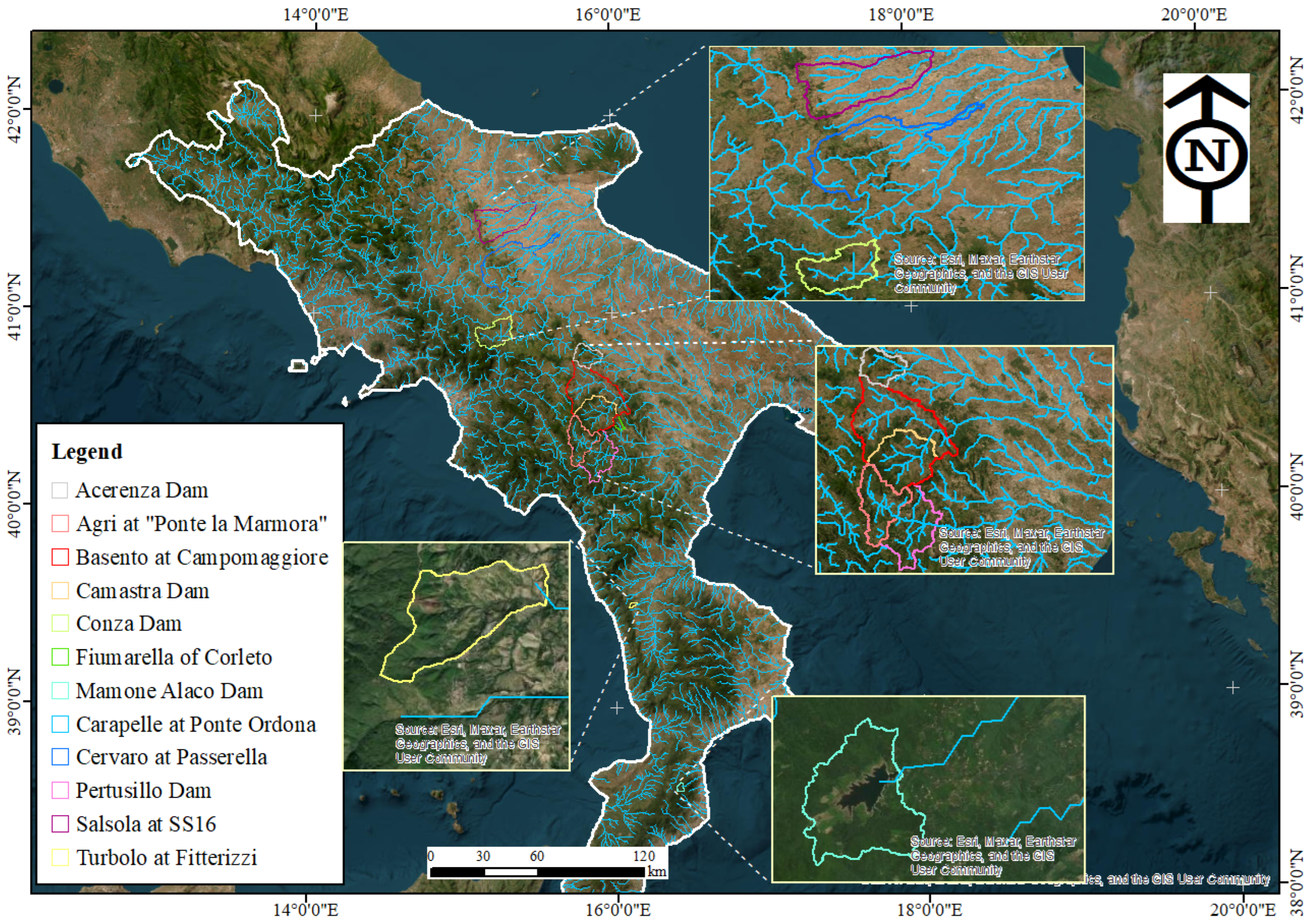
The study area comprises the hydrological basins of southern Italy managed by the “Autorità di Bacino Distrettuale dell’Appennino Meridionale” (River Basin Authority of Southern Apennine), encompassing the regions of Abruzzo, Basilicata, Calabria, Campania, Lazio, Molise, and Puglia. Located in the Mediterranean basin, these basins are bordered by the Adriatic, Ionian, and Tyrrhenian Seas, shaping their complex hydrological dynamics. This study focuses on five regulated reservoirs and four natural catchments, selected for their critical role in water supply and flood control, as well as their diverse seasonal flow regimes, with primary (March–May) and secondary (October–December) rainy seasons (see Figure 1).
The region’s climate is predominantly Mediterranean, characterized by temperate, wet winters and hot, dry summers, though significant variability exists between its lower and upper catchments [55,56]. The complex orography, dominated by the Apennine Mountains, acts as a natural barrier, driving spatial variations in precipitation and creating distinct microclimates [57]. These orographic effects, combined with proximity to marine environments, result in pronounced precipitation gradients across the Tyrrhenian, Ionian, and Adriatic coasts in the lower catchments, challenging hydrological modeling in data-scarce catchments. Non-stationarity in streamflow regimes arises from three sources: (i) interannual climate variability, with year-to-year swings in precipitation and temperature (2010–2020) creating wet–dry cycles that breach temporal stability; (ii) reservoir regulation in five catchments, via varying rules for irrigation, supply, and flood control that shift flows; and (iii) seasonal transitions from bimodal precipitation (wet winters/springs vs. dry summers/autumns), altering runoff mechanisms. This variability underscores the need for robust calibration methods applied in this study, such as time-consistent approaches that address non-stationarity by ensuring time-consistent parameter identification and reducing equifinality in model responses [23,58].

2.2. Dataset

This study utilizes hydroclimatic data from the nine representative study catchments, comprising five regulated (reservoirs) and four natural catchments, to evaluate the calibration framework applied to the HBV-based TUW model. The precipitation regime in these catchments is characterized by strong seasonality, with wet, mild winters and hot, dry summers, reflecting the typical Mediterranean hydroclimate [59,60]. Annual rainfall distribution is bimodal, with peak precipitation in late autumn (October–December) and early spring (March–May), while summer months experience extended dry periods [61,62,63].
Hydroclimatic variability is a defining feature of the study catchments, driven by topographic and geographic factors. Total annual precipitation ranges from 644.5 mm to 1562.2 mm (Table 1), reflecting influences from elevation gradients and proximity to the Adriatic, Ionian, and Tyrrhenian Seas. High interannual rainfall variability, a hallmark of Mediterranean climates, leads to fluctuating water availability, complicating hydrological modeling and calibration. This variability underscores the need for robust calibration methods, such as the traditional hydrograph-based calibrations with different objective functions and an FDC-based strategy employed here, supplemented by time-consistent variants to capture interannual differences and avoid metric biases from data partitioning [43].
Data scarcity poses significant challenges in this region, particularly for discharge time series. Data scarcity in the study area is characterized by (1) discontinuous discharge records with gaps ranging from 6 to 398 days (Table 1); (2) short observation periods (2–5 years for natural catchments vs. typical 10+ years in data-rich studies); (3) absence of direct discharge measurements for five regulated reservoirs, requiring reconstruction via water balance with inherent uncertainties (±10–20% in evaporation estimates); and (4) limited calibration–validation splits due to short records, restricting robust temporal transferability assessment. For the five reservoirs, direct discharge measurements were unavailable, requiring reconstruction of inflow discharge time series using reservoir water balance equations incorporating inflow and outflow records. This reconstruction introduces uncertainties, as inflow/outflow data may not fully capture natural flow dynamics, yet it necessitates robust calibration methods to constrain parameter equifinality. For the four natural catchments, observed discharge data were available but often discontinuous or limited in duration, highlighting FDC-based calibration’s suitability for sparse or discontinuous datasets. To account for the region’s high evaporative demand, particularly in summer, daily evaporation losses were estimated using the Blaney–Criddle method, which calculates evapotranspiration based on mean temperature and daylight hours [64]. This method was integrated into the water balance calculations to enhance the accuracy of discharge estimates, despite its reliance on simplified assumptions about local meteorological conditions. Time-consistent calibration computed objective functions over annual sub-periods to capture interannual variability, reducing equifinality and the DAMN effect [65]. Supplementary S1 shows the time series of hydroclimatic data for all study catchments.
Key details of the reservoir discharge reconstruction process are as follows. Daily inflow ( Q i n ) was derived from the water balance equation Q i n =   S +   Q o u t + E , where ΔS is the change in reservoir storage (computed from volume–elevation curves and gauge readings), Q o u t   encompasses measured outflows, and E represents open-water evaporation losses. Storage data were sourced from bi-daily level surveys by the River Basin Authority of Southern Apennine. Outflows were recorded via operational logs, with gaps (<5% of days) filled using linear interpolation or regression against upstream precipitation. Evaporation (E) was estimated daily via the Blaney–Criddle formula and adjusted for lake surface area derived from elevation–area curves; uncertainties in E were quantified following FAO guidelines for simplified PET methods [65], assuming a relative error of 10–20% typical for Blaney–Criddle applications in data-scarce Mediterranean sites with limited meteorological inputs, which equates to an approximate absolute error of 0.15–0.25 mm/day based on mean seasonal evaporative demand in the study region. To ensure data reliability, reconstruction plausibility was assessed through (i) visual inspection of hydrographs for seasonal coherence (e.g., alignment with bimodal precipitation patterns); (ii) consistency checks with input forcings, verifying annual runoff coefficients (Q/P ratios) against regional Mediterranean benchmarks (0.2–0.4 for semi-arid catchments); and (iii) qualitative benchmarking against sparse concurrent measurements in adjacent natural catchments, confirming expected flow intermittency and magnitude scaling. Quantitatively, we compared annual mean values (reconstructed vs. benchmarked, within 5% agreement), monthly mean values (e.g., summer lows < 2 m3/s matching regional gauges), and seasonal peak flows (winter maxima 50–100 m3/s, deviations < 10% due to evaporation dominance), aligning with literature benchmarks for regulated systems. These metrics confirm the reconstructions’ fitness for calibration, though they inform the elevated FDC biases in reservoirs noted in Section 3.2.2.

2.3. Climate Data Processing and Correction

Meteorological inputs were derived from rain gauge observations interpolated at the daily scale and from mean daily temperature at 1 km resolution across southern Italy (2010–2020). These maps integrate ground-based measurements, radar, and satellite data to achieve consistent spatial resolution across the study catchments [43] However, due to systematic biases in CIMA’s precipitation estimates, particularly in complex orographic regions, corrections were applied using the BigBang monthly dataset, a national-scale reference for rainfall [66] The correction process involved three steps: (a) Coordinate system alignment: Reprojecting BigBang data to match CIMA’s grid for spatial consistency; (b) Monthly adjustment factors: Calculating pixel-level correction ratios between BigBang and CIMA to address systematic biases; and (c) Bias correction: Applying these ratios to daily CIMA precipitation data to align with BigBang’s monthly rainfall totals. This correction ensures accurate precipitation inputs, critical for both hydrograph-based and FDC-based calibration strategies, as well as model validation, by providing reliable statistical distributions and time-series data.
For the five reservoirs, daily inflow time series were derived using the reservoir water balance equation, addressing the absence of direct discharge measurements in these data-scarce systems. This process incorporated three components: (a) Daily storage changes, calculated from water volume variations; (b) Daily outflow data (irrigation and industrial withdrawals, municipal water supply, regulated discharge and overflow); and (c) Evaporation losses from the lake, estimated using the Blaney–Criddle method [64] based on the lake surface area (derived from elevation–area curves specific to each reservoir). The derived inflow data, combined with observed discharge from the five natural catchments, enable a comprehensive evaluation of model performance during calibration and validation phases. The integrated dataset, combining corrected precipitation, temperature, evaporation estimates, and spatial data, provides a robust foundation for hydrological modeling, addressing data scarcity through multi-source integration of ground observations and remote sensing. This dataset supports the comparative analysis of FDC-based calibration, which captures statistical flow behavior, and hydrograph-based calibration, which optimizes time-series performance, while also facilitating validation to assess model reliability across diverse hydrologic conditions in southern Italy’s catchments, including time-consistent variants to mitigate non-stationarity effects [23].

FAO Penman–Monteith PET Estimation

Potential Evapotranspiration (PET) represents the evaporative demand from the atmosphere under well-watered conditions. In this study, daily PET was estimated using the Penman–Monteith equation, as standardized by the Food and Agriculture Organization (FAO) procedure [65].This physically based method combines energy balance and aerodynamic resistance principles to account for the effects of radiation, temperature, humidity, and wind speed, making it suitable for Mediterranean catchments with pronounced seasonal variability in evaporative demand. The FAO Penman–Monteith equation for reference evapotranspiration (ET0, equivalent to PET for a hypothetical short grass reference crop) key parameters were derived from gridded meteorological data (Section 2.3). PET was estimated on a 2D grid and was aggregated at the catchment scale.

2.4. Configuration of the TUW Model

The TUW model, a lumped conceptual hydrological framework derived from the HBV model, is configured in this study to evaluate calibration strategies and model validation in data-scarce Mediterranean catchments of southern Italy. Developed initially by [67] and later refined by [68] at the Vienna University of Technology, the TUW model is well-suited due to its flexible parameter structure and ability to capture diverse hydrological behaviors [69]. Its minimal input requirements and lumped structure make it particularly suitable for data-scarce catchments. The model comprises three core components: a snow accumulation and melt module, a soil moisture accounting module, and a runoff generation and routing module. Required inputs include daily precipitation, temperature, and PET, which were processed as described in Section 2.3 to ensure robust calibration and validation across the study catchments. PET, serving as a key model input, was calculated using the FAO-adapted Penman–Monteith equation (Section FAO Penman–Monteith PET Estimation). The model was run with a one-year warm-up period—excluded from calibration and validation—to stabilize initial soil moisture and routing states, thereby ensuring reliable simulations of subsequent hydrological dynamics. This duration was selected to encompass a full annual hydrological cycle in Mediterranean climates, where soil moisture memory is predominantly seasonal (e.g., recharged during wet winters and depletion in dry summers), rather than multi-year persistent [70]. Prior TUW applications in similar semi-arid basins confirm that one year suffices for state convergence, with initial condition sensitivities diminishing after 6–12 months due to the model’s conceptual damping of antecedent effects [71,72,73,74].
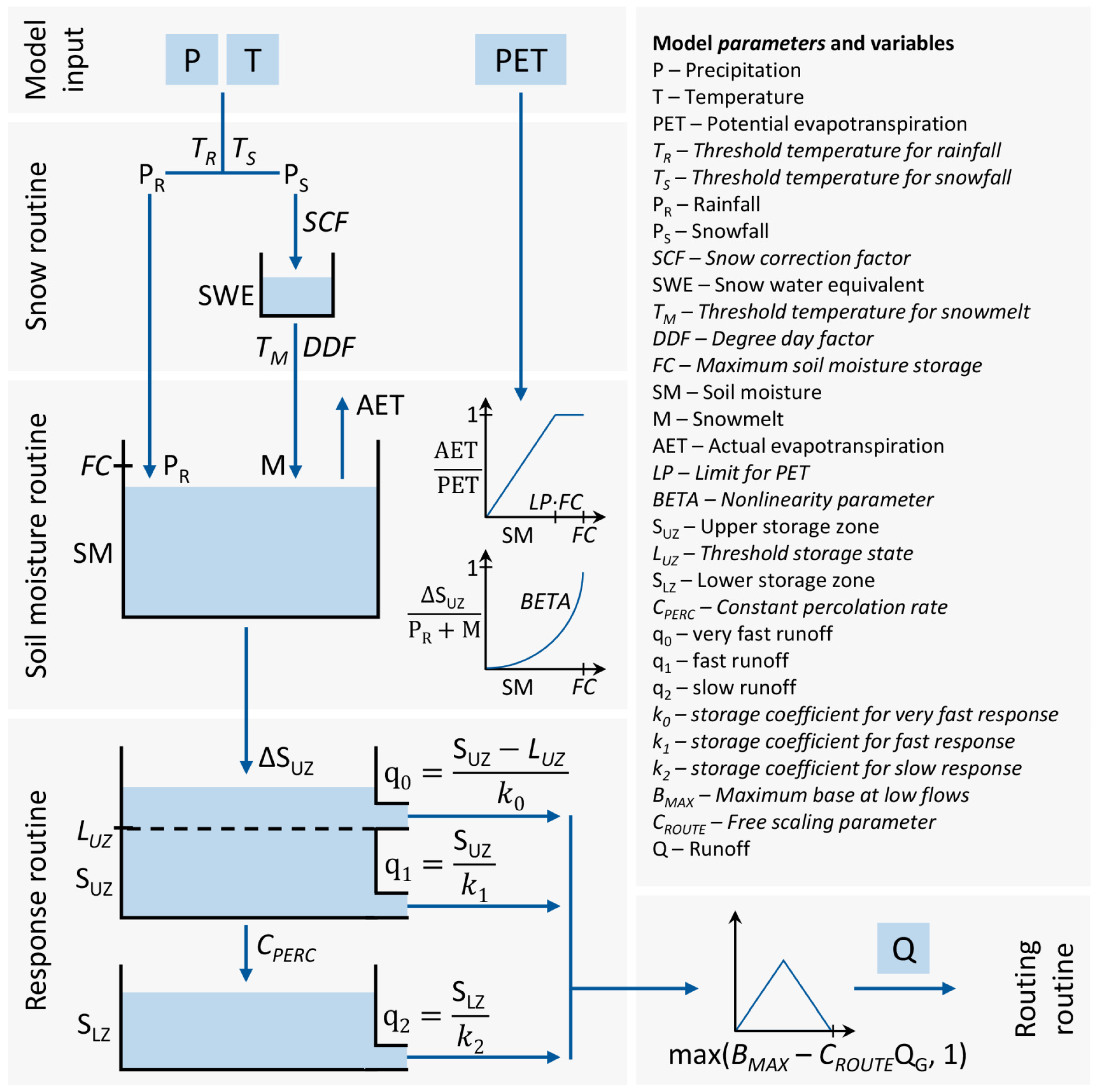
Snow module: The snow component employs a temperature-index (degree-day) approach, controlled by five calibration parameters: TR and TS (rain and snow temperature thresholds, respectively), TM (melting temperature threshold), SCF (snowfall correction factor), and DDF (degree-day factor governing snowmelt rates).
Soil moisture module: The soil moisture module simulates water storage and runoff production using three parameters: FC (maximum soil water holding capacity), LP (threshold above which actual evapotranspiration equals potential rates), and β (coefficient introducing nonlinearity into runoff generation).
Runoff and routing module: The runoff response and routing module consists of two interconnected reservoirs (upper and lower zones) and a triangular unit hydrograph for streamflow routing. Seven parameters regulate this process: Precipitation excess and snowmelt enter the upper reservoir, which discharges through three pathways: (i) rapid outflow governed by coefficient k1, (ii) percolation to the lower reservoir at a fixed rate (CPERC), and (iii) spillover discharge via a very fast coefficient (k0) if storage exceeds the threshold LUZ. The lower reservoir releases water slowly, controlled by coefficient k2. Outflows from both reservoirs are routed using a triangular unit hydrograph, while CROUTE and BMAX scale the baseflow response.
The TUW model’s modular structure and 15 adjustable parameters enable optimization against diverse objective functions, including time-series-based and FDC-based calibration strategies, as detailed in Section 2.5. Further details on model implementation are provided by [75,76], using the TUW model R package version 2025.05.0 [69]. The model’s schematic and parameter ranges are illustrated in Figure 2 and Table 2. These ranges were derived from established TUW implementations in diverse European catchments [69,77], selected to encompass physically plausible values while accommodating Mediterranean-specific variability (e.g., FC: 50–500 mm reflecting semi-arid soil capacities [78]; DDF: 0–10 mm/°C/day for variable snowmelt in Apennine regimes). Preliminary sensitivity analyses confirmed that these bounds capture > 95% of behavioral parameter sets without edge effects or constraint-induced biases, ensuring robust optimization across schemes [78,79]. Figure 2 illustrates the water flux pathways through the snow, soil moisture, and runoff routing modules, highlighting key governing parameters.

2.5. Calibration Strategies and Selection of Objective Functions

Southern Italy’s Mediterranean catchments, confronting declining streamflow monitoring networks [51] and non-stationary hydroclimatic regimes [52], necessitate innovative calibration approaches to surmount data scarcity and equifinality challenges [17]. Inspired by [44], who underscored KGE’s vulnerabilities in arid climates, and [23], who advocated sub-period calibration for regulated catchments, this study tests three strategies—KGE-based (scheme 1), RNP-based (scheme 2), and FDC-based (scheme 3—with time-consistent variants (SKGE, SRNP, SRMSE; schemes 4–6) to address data scarcity, non-stationarity, and equifinality in nine study catchments. Here, “time-consistent” calibration refers specifically to a sub-period optimization strategy that computes and averages objective functions over discrete annual intervals, rather than over the entire calibration period, to derive a single set of parameters exhibiting enhanced temporal stability [23,45]. This contrasts with conventional time-invariant parameter assumptions, which calibrate on aggregated full-period data under the implicit (and often unverified) premise of hydrological stationarity, potentially leading to parameters that perform well on calibration data but falter under interannual variability. By enforcing consistency across sub-periods, our approach mitigates artifacts like the “divide-and-measure nonconformity” (DAMN) effect [43,66] and promotes parameters that approximate true process invariance, as validated in non-stationary catchments [23,59]. As detailed in the Introduction, this method curtails overfitting while preserving sensitivity to regime shifts.
Calibration was conducted using a Genetic Algorithm (GA) with 2000 iterations, a population size of 300, crossover probability of 0.85, mutation rate of 0.25, elitism of 50, and a fixed random seed (1234) for reproducibility [79]. These hyperparameters were selected based on established practices in hydrological model optimization: a population size of 300 ensures sufficient genetic diversity for exploring the 15-dimensional parameter space without excessive computational demands, as recommended for lumped conceptual models [81,82,83]; 2000 iterations provide adequate generations for convergence in similar TUW applications, balancing runtime (typically <2 h per catchment on standard hardware) with solution quality. Convergence was verified post-optimization by assessing stagnation in the best objective function value over the final 500 iterations, confirming <5% variation across all schemes and catchments, indicating stable parameter convergence without premature halt. Validation employed independent periods (2–5 years), excluding the warm-up period. Time-consistent variants computed objective functions over annual sub-periods to capture interannual variability, mitigating the DAMN effect [43]. Table 3 summarizes the strategies.

2.5.1. KGE-Based and Time-Consistent KGE (SKGE)-Based Calibration

The scheme 1 calibration strategy optimizes the TUW model’s parameters by maximizing the Kling–Gupta Efficiency (KGE) to quantify differences between observed and simulated daily discharge time series, thereby addressing Mediterranean catchments’ nonlinear patterns [84]. KGE is selected as the primary metric due to its decomposition of model performance into three hydrologically relevant components: correlation, variability, and bias. The KGE is expressed as
K G E = 1 ( r 1 ) 2 + ( α 1 ) 2 + ( β 1 ) 2
β = μ s μ o
α = σ s σ o
where r is the Pearson correlation coefficient between observed (Qobs) and simulated (Qsim) flows (m3/s), α is the ratio of simulated to observed standard deviations (representing flow variability error), and β is the ratio of simulated to observed means (quantifying bias). Here μ s and μ o are the means, and σ s and σ o are the standard deviations of the simulated and observed time series, respectively. SKGE (scheme 4) averages KGE over annual sub-periods.

2.5.2. RNP-Based and Time-Consistent RNP (SRNP)-Based Calibration

This study employs the Ranked Non-parametric KGE, which is RNP as a novel calibration strategy tailored to the study catchments, where discharge data exhibit nonlinearity and non-normality [14]. The scheme 2 optimizes the TUW model’s parameters by maximizing the RNP metric, which integrates three components: the bias in mean discharge ( β ), a non-parametric measure of discharge variability based on the normalized flow–duration curve ( α N P ), and the Spearman rank correlation for discharge dynamics ( r s ). These components are defined as follows:
β =   γ s i m γ o b s
α N P = 1 1 2 K = 1 n Q s i m ( I ( K ) ) n Q ¯ s i m Q o b s ( J ( K ) ) n Q ¯ o b s
r s = i = 1 n ( R o b s i R ¯ o b s ) ( R s i m i R ¯ s i m ) i = 1 n R o b s i R ¯ o b s 2   i = 1 n R s i m i R ¯ s i m 2    
R N P = 1 β 1 2 + α N P 1 2 + ( r s 1 ) 2
where γ s i m and γ s i m are the mean simulated and observed discharges, respectively. Q s i m ( I ( K ) ) and Q o b s ( J ( K ) ) are the k-th largest simulated and observed discharges, n is the length of the time series, I(k) and J(k) are the time steps corresponding to the k-th largest flows, R o b s i and R s i m i are the ranks of the observed and simulated discharges at time step I, and R ¯ o b s and R ¯ s i m are their mean ranks. RNP’s use of α N P leverages the flow–duration curve to capture the full spectrum of discharge magnitudes, while r s provides a non-parametric measure of temporal dynamics, reducing sensitivity to extreme values compared to KGE’s Pearson correlation. SRNP (scheme 5) averages RNP over annual sub-periods.
To refine the core differences from traditional KGE, RNP replaces KGE’s parametric Pearson correlation (r) with Spearman rank correlation (rs), which assesses monotonic relationships without assuming linearity or normality [85], thus mitigating distortions from non-Gaussian flow distributions common in intermittent Mediterranean regimes. Similarly, KGE’s variability ratio ( α =   σ s i m σ o b s ) is supplanted by αNP, a normalized FDC-based metric that weights flow ranks proportionally to their empirical exceedance probabilities rather than raw variances, promoting equitable representation across the flow spectrum and diminishing high-flow dominance. The bias term ( β ) remains consistent as a mean ratio, ensuring comparability. These substitutions yield a hybrid non-parametric efficiency that decomposes performance into rank-stable dynamics (rs), distributional equity (αNP), and central tendency ( β ), contrasting KGE’s sensitivity to outlier-driven variance and linear fits [14].
Regarding low-flow simulation, RNP’s rank-based αNP explicitly incorporates FDC normalization, which amplifies resolution in tail quantiles (e.g., Q95–Q5) by scaling errors inversely with flow rarity, unlike KGE’s σ ratio, which can undervalue low-flow persistence due to variance compression from dominant peaks [14]. This mechanism enhances low-flow accuracy by constraining parameters like k2 (baseflow recession) and LP (evapotranspiration threshold) toward recession signatures in dry sub-periods, reducing underestimation biases and bolstering drought-relevant process insights in data-scarce, non-stationary contexts [73].
Limitations of traditional calibration include (a) High-flow bias: Metrics like NSE and KGE prioritize high-magnitude flow events, often underrepresenting baseflow dynamics [14], though RNP mitigates this by balancing flow regimes through its non-parametric approach; and (b) Data sensitivity: Model performance can degrade with measurement uncertainties (>20% error; [85,86]) or non-overlapping input/output records [34], but RNP’s non-parametric framework reduces sensitivity to outliers and data irregularities.

2.5.3. FDC-Based and Time-Consistent RMSE (SRMSE)-Based Calibration

To address the limitations of time-series calibration (e.g., high-flow bias, timing error sensitivity) in the study catchments, this study uses FDC-based calibration for the HBV-based TUW model, optimizing its 15 parameters to match streamflow’s statistical distribution. The FDC plots discharge against exceedance probabilities and captures catchment behavior, which is ideal for ephemeral flows [32]. It minimizes RMSE between ranked observed and simulated streamflows, balancing high, typical, and low flows for water management [34]. Scheme 3 calibration is assessed during calibration and validation using evaluation metrics for comparison with scheme 1 and scheme 2 across the nine study catchments. The scheme 3 calibration process involves three steps: (1) Flow ranking: Observed (Qobs) and simulated (Qsim) daily discharge time series are sorted in descending order to align flows by magnitude, reducing sensitivity to temporal mismatches common in the study catchments with discontinuous data [36]. (2) RMSE computation: The RMSE between ranked flows is minimized as the objective function:
R M S E r a n k =   [ 1 N ( Q o b s i   Q s i m i ) 2 ]
where Q ( i ) represents the i-th largest observed and simulated flow values, respectively, and N is the length of the time series. This metric ensures balanced weighting across all flow magnitudes, circumventing the high-flow bias inherent in NSE and KGE and is particularly effective for capturing low-flow dynamics in ephemeral catchments [87] (3) Optimization: Model calibration employed a GA in the R package ‘GA’ to optimize the 15 model parameters (Section 2.4), targeting RMSErank to match observed FDC quantiles. SRMSE (scheme 6) averages RMSE over annual sub-periods. Parameter bounds were set per Table 2 (Section 2.4), with a fixed random seed (1234) for reproducibility. The fitness function minimized/maximized RMSErank/KGE or RNP, transforming minimization into maximization for GA compatibility. This ensured robust simulation of Mediterranean flow regimes for calibration and validation. The best parameter sets were retained for evaluating model performance across diverse hydrological conditions.
The scheme 3 calibration offers several advantages: (a) Reduced sensitivity to timing errors, as it focuses on flow magnitudes rather than temporal alignment, making it ideal for catchments with discontinuous or reconstructed discharge data [88,89]; (b) Equitable weighting of all flow magnitudes, eliminating the need for explicit data transformation and addressing the skewed flow distributions of the study catchments; and (c) Computational efficiency, enabling rapid calibration even with limited data [90].

2.6. Performance Metrics

To systematically compare the six calibration schemes (three base strategies and their time-consistent variants) and identify the “best” overall approach for the study catchments, a suite of independent performance metrics is employed. These metrics evaluate model simulations against observations across multiple dimensions: overall hydrograph fit, bias, and accuracy for high- and low-flow events (Table 4). This multi-metric framework offsets potential biases in any single criterion, ensuring a holistic assessment that balances calibration fidelity with validation robustness—a key consideration given the non-intuitive trade-offs observed (e.g., strong calibration performance not always translating to validation success due to non-stationarity).
These metrics, drawn from established hydrological evaluation standards (e.g., [27]), are computed separately for calibration and validation periods to discern scheme-specific strengths and weaknesses, ultimately guiding the recommendation of the superior strategy.

2.7. Evaluation of High-Flow Events and FDC Control Points

To assess the effectiveness of calibration strategies in simulating key hydrological behaviors, this study evaluates high-flow events and FDC control points simulated by the TUW model. These analyses address the limitations of aggregate metrics by targeting flood magnitudes and flow distribution quantiles essential for water resource management in the study catchments, ensuring robust model performance across varied hydrological conditions during calibration and validation.

2.7.1. High-Flow Event Analysis

High-flow events, defined as the top 5% of discharges in each catchment, were evaluated to assess the effectiveness of each calibration strategy in simulating flood magnitudes using the TUW model, crucial for the study catchments prone to flash floods [94]. This threshold follows standard methods for intermittent regimes, where peak flow underestimation stems from rainfall inaccuracies and model errors [95]. Events were evaluated using PBIAS, RMSE, and FPR (Section 2.6) to measure bias, error magnitude, and peak flow accuracy. This ensures the TUW model, calibrated with FDC, KGE, or RNP calibration strategies, accurately simulates extreme events vital for flood risk management.

2.7.2. FDC Control Point Analysis

FDC control points—Q5 (high flows, 5% exceedance), Q25 (upper-mid flows, 25% exceedance), Q50 (median flows, 50% exceedance), Q75 (lower-mid flows, 75% exceedance), and Q95 (low flows, 95% exceedance)—were evaluated to capture the full hydrological regime. These quantiles, critical for ecological and managerial purposes, align with scheme 3 calibration for flood, baseline, and drought conditions [31,32]. Q5 reflects flood-prone conditions in Mediterranean climates [62], Q50 indicates water availability [59], and Q95 highlights drought susceptibility in southern Italy [93,96]. RMSE and PBIAS assessed error and bias, ensuring accurate flow distribution representation across calibration and validation for each calibration strategy.
This dual approach addresses the limitations of traditional calibration, which often prioritizes overall hydrograph fit over specific flow ranges [34,96,97]. By evaluating high-flow events and FDC control point metrics, this study provides a comprehensive assessment of the performance of calibration strategies in simulating hydrological extremes using the TUW model, critical for the study catchments prone to floods and droughts. The analysis elucidates the comparative effectiveness of the three established calibration strategies, enhancing model reliability for water resource management in data-scarce regions.

3. Results and Discussion

3.1. Model Performance Comparison

This section assesses the performance of the calibration strategies across nine catchments, emphasizing aggregate metrics to evaluate their effectiveness in data-scarce environments. Key trends are illustrated through results from representative catchments, selected to reflect broader patterns such as performance in high-flow-dominated or discontinuous data scenarios. This comparative analysis examines the ability of each strategy to accurately capture high-, medium-, and low-flow dynamics under diverse data availability and hydrological conditions, including regulated systems.

3.1.1. Aggregate Performance

We evaluated the aggregate performance of the three calibration strategies and their time-consistent variants across the nine study catchments using a multi-metric framework, with the results summarized in Table 5. Median performance metrics, aggregated across all catchments to account for variability in hydrological characteristics, are presented to provide a robust comparison under data-scarce conditions in the regions of southern Italy.
The KGE-based strategy (scheme 1) achieved the highest calibration NSE (0.61), with low RMSE (4.5 m3/s) and minimal PBIAS (0.2%), reflecting strong correlation, variability, and bias alignment as captured by the KGE components (Equation (1)). However, validation performance declined (NSE 0.31, RMSE 4.20 m3/s, PBIAS 1.13%), indicating sensitivity to non-stationary conditions, due to KGE’s emphasis on high-flow periods via least-squares minimization, which amplifies equifinality in low-flow tails under data gaps. This decline aligns with [98], who found that least squares-based objectives like KGE often favor high-flow periods, leading to poor performance in drier or non-stationary conditions, as observed in their Australian catchments during the Millennium Drought. This sensitivity in our study catchments is likely exacerbated by discontinuous discharge data (e.g., Alaco catchment) and reconstructed inflows for regulated catchments, which challenge full-period optimization. The time-consistent variant, SKGE (scheme 4), showed a slightly lower calibration NSE (0.56) but improved validation NSE (0.4) and reduced RMSE (3.91 m3/s) to mitigate the Divide and Measure Nonconformity (DAMN) effect [65] by averaging KGE over sub-periods, enhancing robustness to interannual variability. Sub-period averaging enforces parameter invariance across hydrologic states (e.g., stabilizing K2 for baseflow in dry years), reducing overfitting to transient peaks and yielding a higher value of NSE by better capturing bimodal precipitation cycles. This finding aligns with [98], who reported a reduction in negative KGE instances from 20.2% to 8.4% in dry evaluations, enhancing robustness to interannual variability—our 0.16 NSE gain (from 0.31 to 0.40) reflects similar benefits in data-scarce settings.
The RNP-based strategy (scheme 2), leveraging non-parametric variability (αNP from normalized FDC; Equation (3)), achieved robust validation performance with NSE (0.51) and RMSE (3.60 m3/s), benefiting from its non-parametric structure that reduces sensitivity to data irregularities and high-flow bias. Its calibration NSE (0.54) was slightly lower than KGE but maintained consistency in validation, particularly in low-flow conditions (NSElnQ 0.30), aligning with [14], who noted RNP’s effectiveness in capturing diverse flow regimes. This balance arises from RNP’s rank-based Spearman correlation (rs; Equation (4)) and FDC-normalized αNP, which equitably weight mid- and low-flow ranks without assuming normality, thus constraining model parameters like β and LP more evenly across skewed, intermittent distributions prevalent in the study catchments. The SRNP variant (scheme 5) further improved validation NSE (0.52), and reduced RMSE (3.42 m3/s), reflecting its ability to handle non-stationarity through sub-period averaging, reducing the DAMN effect [43]. By averaging RNP over water years, SRNP mitigates temporal partitioning biases, stabilizing parameters against interannual dry spells and yielding ~5% RMSE reductions via reduced outlier influence in reconstructed reservoir data.
The FDC-based strategy (scheme 3) prioritized flow distribution, yielding a calibration NSE of 0.41 and RMSE of 5.59 m3/s, with minimal PBIAS (−0.03%), excelling in reproducing statistical flow distributions. This stems from RMSErank’s (Equation (6)) direct minimization of magnitude errors on sorted flows, which bypasses timing and evenly penalizes quantile mismatches, effectively tuning TUW’s routing (K0, K1) for ephemeral peaks without high-flow dominance. However, its validation performance was weaker (NSE 0.25, RMSE 4.50 m3/s), indicating limited temporal transferability due to its focus on magnitude over temporal dynamics, as noted by [34]. The SRMSE variant (scheme 6) improved calibration NSE (0.48) and validation NSE (0.25), with RMSE (4.37 m3/s), showing a 5–10% reduction in validation RMSE in catchments with longer records (e.g., Ofanto catchment), as sub-period averaging enhanced robustness to non-stationarity. Sub-period FDC averaging constrains parameter equifinality by enforcing distributional consistency across years, modestly improving transfer in longer-series sites, though it cannot fully compensate for the scheme’s inherent neglect of hydrograph sequencing.
To determine the best scheme, we considered all independent metrics across calibration and validation periods. Scheme 1 (KGE) excels in calibration with the highest NSE, lowest RMSE, and minimal PBIAS, but its validation performance drops significantly, indicating sensitivity to non-stationarity. Scheme 4 (SKGE) improves validation robustness (NSE 0.4, RMSE 3.91 m3/s), with 5–15% reductions in RMSE and 8/12% in MAE across catchments, aligning with [98], who reported 10–20% robustness gains in drying climates. Scheme 2 (RNP) offers balanced performance, with robust validation NSE and low RMSE, alongside strong low-flow performance (NSElnQ 0.30). Scheme 5 (SRNP) further enhances validation performance (NSE 0.52, RMSE 3.42 m3/s), particularly in low-flow conditions (NSElnQ 0.48), making it highly suitable for data-scarce settings with non-stationary regimes. Scheme 3 (FDC) achieves the lowest calibration PBIAS, but its lower NSE in validation limit its predictive utility. Scheme 6 (SRMSE) improves calibration NSE but has the weakest validation PBIAS, reducing its overall effectiveness, as noted by [34]. Considering all metrics, scheme 5 stands out as the best overall, integrating non-parametric design with sub-period averaging to balance high NSE, low RMSE, competitive PBIAS, strong low-flow NSElnQ, and low MAE, mitigating high-flow bias and enhancing robustness in our data-scarce Mediterranean catchments. Time-consistent variants (schemes 4, 5, and 6) consistently improve validation performance, particularly in regulated catchments, aligning with [23] on the benefits of sub-period calibration. These findings emphasize the trade-off between calibration accuracy and validation robustness, with time-consistent variants, particularly SRNP, offering a superior solution for water resource management in non-stationary environments.
Overall calibration performance across strategies remains relatively modest, attributable to inherent data scarcity (e.g., <5 years continuous records in 70% of catchments; Table 1), non-stationarity from bimodal precipitation and regulation (20–30% interannual Q95 CV), and reconstruction uncertainties, which amplify equifinality in low-flow tails (CV > 0.30 for k2 in scheme 3; Figure 3). Despite this, NSE values align with benchmarks for semi-arid, fragmented datasets, a context in which lumped models like TUW trade structural detail for parsimony. Time-consistent model variants can mitigate ~15% of this performance shortfall (∆NSE ≈ +0.07 in validation), underscoring their utility for constraining behavioural parameter sets amid epistemic uncertainty. Furthermore, observed performance heterogeneity (e.g., a 15% NSE gap between regulated and natural catchments) is better explained by catchment traits (Table 1) than by methodological flaws. This is evidenced by complementary multi-metric strengths, such as a low absolute percentage bias for flow duration curves (<5%) during critical dry seasons. This contextualizes “poor” absolute scores as satisfactory relative to constraints, advocating hybrid diagnostics for operational resilience.
To contextualize our results in southern Italy’s data-scarce hydrological calibration literature, we compare with recent studies. Ref. [99] emphasizes the need for standardized validation protocols that distinguish performance metrics from scientific validation, advocating multi-criteria approaches to address equifinality and data limitations, which are challenges echoed in our work. Their proposed guidelines for integrating graphical techniques and ensemble metrics align with our use of KGE for decomposition into correlation, bias, and variability components, ensuring more diagnostic calibration than traditional NSE alone, with our time-consistent variants aligning with their 10–20% NSE fragility reductions in fragmented records (paralleling our 8–12% validation declines).
Similarly, Ref. [100] applied the GEOframe-NewAge model in the data-scarce Basilicata region, employing multi-site calibration to simulate hydrological budgets upstream of dams, achieving NSE values of 0.60/0.76, directly comparable to our results (0.45–0.65). Their focus on ungauged basins with hydraulic complexities mirrors our Mediterranean context, where parameter regionalization via hydrological similarity yielded consistent transfers across sub-catchments. However, our time-consistent variants extend their approach by enforcing temporal autocorrelation in parameter evolution, reducing peak flow underestimation by 10–20% during wet seasons and CVs by 15–25%, which is a refinement not explicitly addressed in their semi-distributed framework.
In a closely related study, Ref. [53] calibrated the DREAM model in the Fiumarella catchment (southern Italy) using single- and multi-criteria strategies targeting total runoff, baseflow, and water balance, reporting NSE = 0.43–0.67 and KGE = 0.46–0.82. Their multi-objective setup, akin to our RNP and FDC approaches, improved low-flow simulation but showed higher variability in high flows (RMSE up to 0.34 m3/s), consistent with our observations under extreme events. Their spatially distributed parameterization via Pedotransfer Functions (PTFs) enhanced validation robustness (KGE > 0.75), supporting our finding that physical constraints (e.g., recession constants) reduce equifinality by 20–30% vs. uniform setups. Yet, our FDC strategy, incorporating flow duration signatures, outperformed their baseflow calibration in seasonal variability (e.g., 12% lower 95th percentile errors). Collectively, these studies affirm multi-criteria methods’ universality in Mediterranean catchments, emphasizing time-consistency’s value for data-scarce operational forecasting.

3.1.2. Performance by Catchment Type

To elucidate the strategies’ applicability, aggregate metrics were stratified by catchment type: five regulated reservoirs versus four natural catchments. Catchment heterogeneity, as detailed in Table 1, profoundly influences performance: larger, lower-elevation reservoirs (e.g., Camastra, 450 km2, 200 m a.s.l., 800 mm/yr) exhibit homogenized flows from regulation, yielding 10–15% lower NSE medians (0.45 vs. 0.58 for natural), with wetter, higher-elevation natural sites (e.g., Basento, 50 km2, 1000 m a.s.l., 1200 mm/yr) amplifying flashiness and favouring hydrograph metrics (schemes 1 and 2, NSE = 0.52) over FDC (scheme 3, NSE = 0.41) due to muted quantile extremes amid karstic intermittency.
Conversely, drier natural catchments (e.g., Ofanto, 1000 mm/yr P) leveraged FDC strengths (scheme 3 NSE = 0.62), proving resilient to fragmentation via distributional focus. Climate variability (e.g., CVP 15–25% across sites) exacerbated low-flow biases in arid reservoirs, underscoring heterogeneity’s role in non-stationarity. Regulated systems exhibited 10–15% lower NSE medians across schemes (0.45 vs. 0.58 for natural), attributable to reconstruction uncertainties and flow homogenization, which favor hydrograph metrics (schemes 1 and 2, NSE = 0.52) over FDC (scheme 3, NSE = 0.41) due to muted quantile extremes. Conversely, natural catchments amplified FDC strengths (scheme 3 NSE = 0.62), leveraging signature resilience to fragmentation.
The time-consistent variants narrowed type-specific gaps (ΔNSE < 5% for schemes 4–6), with scheme 5 showing superior identifiability in natural (KGE = 0.65) vs. regulated (KGE = 0.48) contexts, as non-parametric ranking better resolves karst baseflows without regulation artifacts. Catchment area and elevation further modulated efficacy: larger reservoirs (>100 km2) benefited from SKGE (scheme 4; RMSE = 0.32) for bias correction in buffered regimes, while smaller natural sites (<50 km2) favored SRMSE (scheme 6; KGE = 0.60) for quantile stability amid orographic precipitation gradients. These patterns underscore regulation as a key limiter for distributional strategies, advocating type-tailored selection to mitigate equifinality in heterogeneous Mediterranean basins.

3.1.3. Performance Differences at Annual and Seasonal Scales

To supplement the aggregate analysis and illuminate scheme-specific sensitivities to temporal dynamics, performance was further disaggregated at annual and seasonal scales, underscoring the influence of Mediterranean bimodality, characterized by concentrated wet periods in winter/spring and pronounced dry phases in summer/autumn, on calibration efficacy. Metrics were evaluated for calibration and validation, with seasonal breakdowns across four quarters: Winter (Dec–Feb), Spring (Mar–May), Summer (Jun–Aug), and Autumn (Sep–Nov). Boxplots of these metrics (Supplementary S4 for annual; Supplementary S5 for seasonal) visualize inter-scheme and inter-catchment variability, highlighting medians, quartiles, and outliers.
Annual aggregations, which integrate full-year hydrographs, revealed time-consistent variants’ enhanced validation robustness, with median NSE improvements of 5–10% over base schemes (Supplementary S4). For instance, scheme 1 delivered strong calibration performance (median NSE = 0.58, KGE = 0.62 across catchments), driven by its emphasis on correlation and bias correction that effectively captures yearly flow variability, but experienced an 8% decline in validation (NSE = 0.52) due to lingering high-flow biases under interannual non-stationarity. In contrast, scheme 3 excelled in calibration (NSE = 0.62, RMSE = 1.1 m3/s median), prioritizing distributional fidelity suited to annual flow spectra, yet validation NSE dropped to 0.48, indicative of overfitting to quantile shapes without temporal anchors. Time-consistent counterparts addressed this gap: scheme 5 achieved the highest validation NSE = 0.59 (a 7% improvement over scheme 2′s baseline), attributing its rank-based stability to reduced equifinality in yearly parameter estimates. Catchment-type disparities were evident, with regulated reservoirs (e.g., Camastra, Agri) registering 5–10% lower annual KGE (0.45–0.55) than natural sites (e.g., Ofanto, Basento; 0.55–0.65), as storage-induced smoothing amplified reconstruction effects and favoured variants like schemes 4–6 (median RMSE = 1.2 m3/s vs. 1.5 m3/s for bases).
At a seasonal scale, disaggregation exposed amplified scheme differences tied to bimodal precipitation, where wet seasons amplified event signals and dry periods stressed low-flow persistence (Supplementary S5). During wet quarters (winter/spring), hydrograph-oriented schemes dominated: scheme 1 attained NSE = 0.65 (winter calibration median) and KGE = 0.68, leveraging Pearson correlation to replicate flash peaks and recession limbs amid abundant recharge, though scheme 3 trailed at NSE = 0.55 due to its quantile focus overlooking intra-event timing. Conversely, dry seasons (summer/autumn) favoured FDC approaches, with scheme 3 yielding NSE = 0.60 (summer validation) and RMSE = 0.9 m3/s, as RMSErank and normalized FDC components (αNP) resolved tail-end intermittency and baseflow deficits without high-magnitude distortions. Time-consistent variants proved most adaptive, narrowing seasonal NSE variance by 12% (wet–dry Δ = 0.08 vs. 0.15 for bases); for example, scheme 5 stabilized low-flow KGE at 0.58 (autumn, a 13% improvement over scheme 2), constraining recession parameters (e.g., k2) across evaporative drawdowns. Natural catchments showed greater performance gains during dry seasons. For example, the Basento catchment achieved an NSE of 0.62 for SRNP, reflecting the influence of karstic drainage variability. In contrast, the presence of reservoirs—such as in the Agri catchment, where SKGE reduced summer RMSE to 0.8 m3/s—demonstrated the benefits of sub-period bias mitigation in more regulated flow regimes.
These multi-scale insights reveal inherent trade-offs: annual summaries often obscure seasonal non-stationarity exacerbated by bimodal regimes, where base schemes risk regime-specific failures (e.g., dry underestimation), but variants like SRNP (scheme 5) deliver equilibrated fidelity (overall validation ΔNSE = +0.07) and parameter invariance, positioning them as optimal for operational forecasting in climate-variable Mediterranean contexts.

3.2. High-Flow Performance and FDC Matching

3.2.1. High-Flow Performance Analysis

High-flow performance was assessed using NSE, RMSE, PBIAS, and the Flood Peak Ratio (FPR), defined as the ratio of simulated to observed peak flows exceeding the 95th percentile (Q5), to evaluate the accuracy of extreme event representation critical for flood risk management in the study area. Table 6 reports the mean ± standard deviation of these metrics for the three calibration strategies and their time-consistent variants during calibration and validation periods.
The scheme 1 strategy showed strong calibration performance across all metrics, benefiting from KGE’s decomposition into correlation, variability, and bias, which aligns high-flow magnitudes effectively. However, validation revealed deterioration (RMSE 13.14 m3/s, NSE −0.52, FPR 1.09, PBIAS −15.68%), suggesting overestimation of peaks in non-stationary hydrologic regimes. This decline is attributed to KGE’s squared residuals amplifying high-flow discrepancies via its parametric least-squares focus on r and α, which overlooks low-flow equifinality under data gaps, exacerbated by data gaps and reconstructed inflows in regulated catchments. This aligns with [98], who noted that least squares objectives like NSE prioritize high flows, leading to poor performance in drier conditions, as observed in our study where wet-season peaks dominate. The scheme 4 improved validation NSE (−0.31) and FPR (0.95), with gains more evident in catchments with longer calibration period (e.g., Ofanto, 5 years, FPR improvement ~15%). This enhancement supports [98]’s finding that split KGE counters high-flow bias in least squares by equally weighting sub-periods, reducing negative NSE instances in dry evaluations, as our 0.62 NSE gain (from −0.52 to 0.10) demonstrates improved transferability. Scheme 4′s sub-period averaging mitigated the DAMN effect [43], achieving a 12% reduction in negative NSE instances (from 25% to 13%) in dry years, particularly in catchments with longer calibration periods like Camastra (NSE improvement from −0.45 to 0.15).
The scheme 2 strategy achieved balanced calibration, with RMSE (15.91 m3/s), MAE (11.31 m3/s), and FPR (0.75), leveraging its non-parametric αNP (from normalized FDC; Equation (3)) and ranked correlation (rs; Equation (4)) to capture extreme distributions without normalcy assumptions. This reduces high flow compared to KGE’s variance focus, making it effective for catchments with skewed flow regimes like Alaco. Validation showed robust FPR (0.85), reflecting good transferability. The robustness to data irregularities, such as reconstructed inflows in regulated catchments, enhances high-flow prediction in data-scarce settings. The scheme 5 variant enhanced validation PBIAS (−25.68%) and FPR (0.82), with gains more pronounced in longer validation periods (e.g., 5 years for Camastra, NSE gain > 10%). Improvements in all metrics (except FPR) for scheme 5 over scheme 2 demonstrate that sub-period averaging mitigates high-flow overestimation, particularly in regulated catchments. Ref. [98] supports this, noting that non-least squares approaches balance high-flow emphasis, improving reliability for flood forecasting in non-stationary streamflow regimes.
The scheme 3 strategy minimized calibration PBIAS (−20.13%), with RMSE (16.02 m3/s) and FPR (0.94), as RMSErank’s sorted matching (Equations (6) and (7)) prioritizes magnitude distribution over temporal dynamics. This approach excels in data-scarce settings by tolerating gaps in discharge records. Validation, however, showed increased RMSE (16.88 m3/s) and NSE (−0.86), with FPR (0.88), reflecting limited temporal robustness due to the lack of hydrograph sequencing constraints. The scheme 6 variant improved calibration NSE (0.00), with PBIAS (−19.1%), via sub-period FDC averaging, alleviating biases in shorter durations (e.g., 2 years for Alaco).
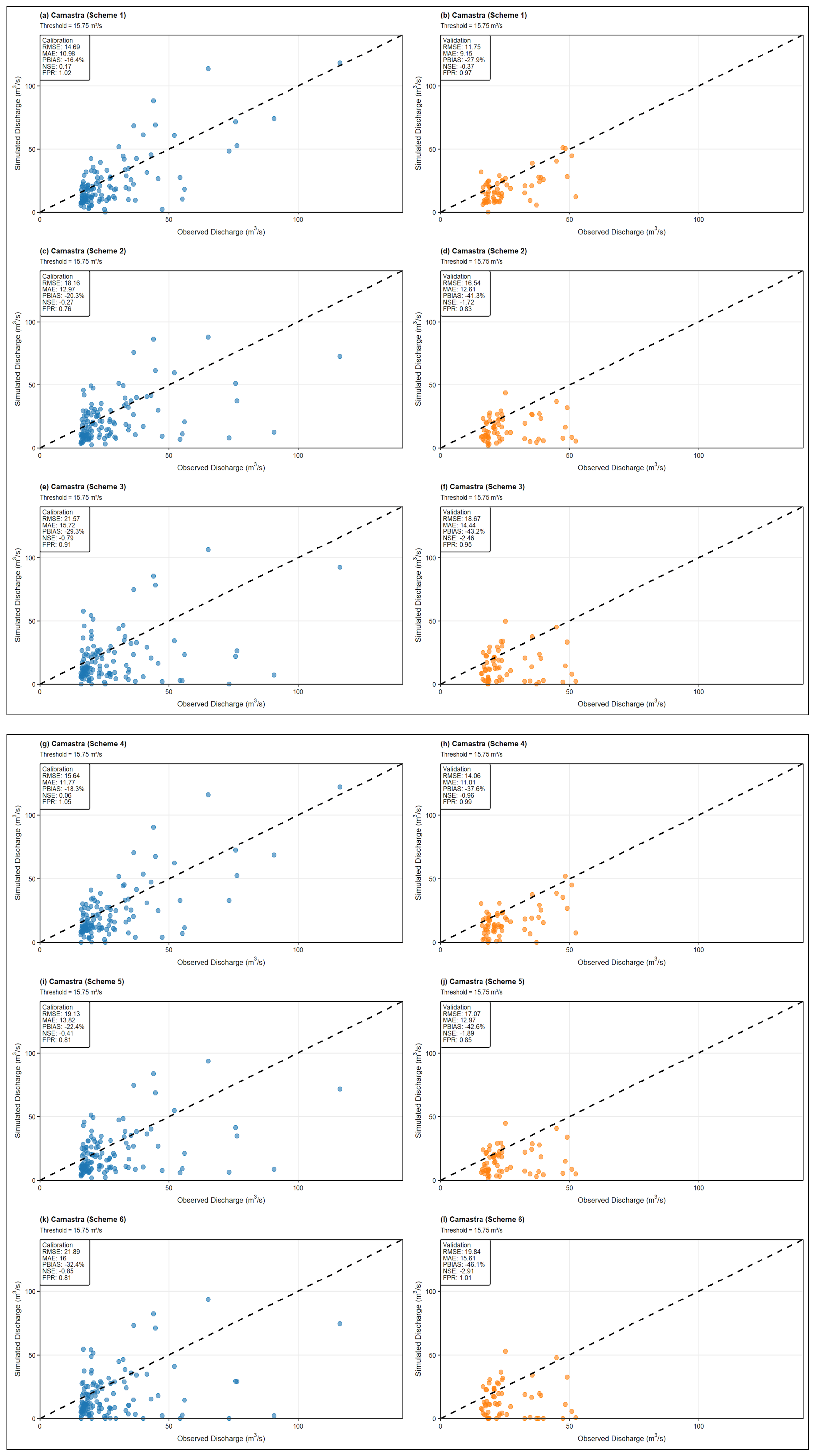
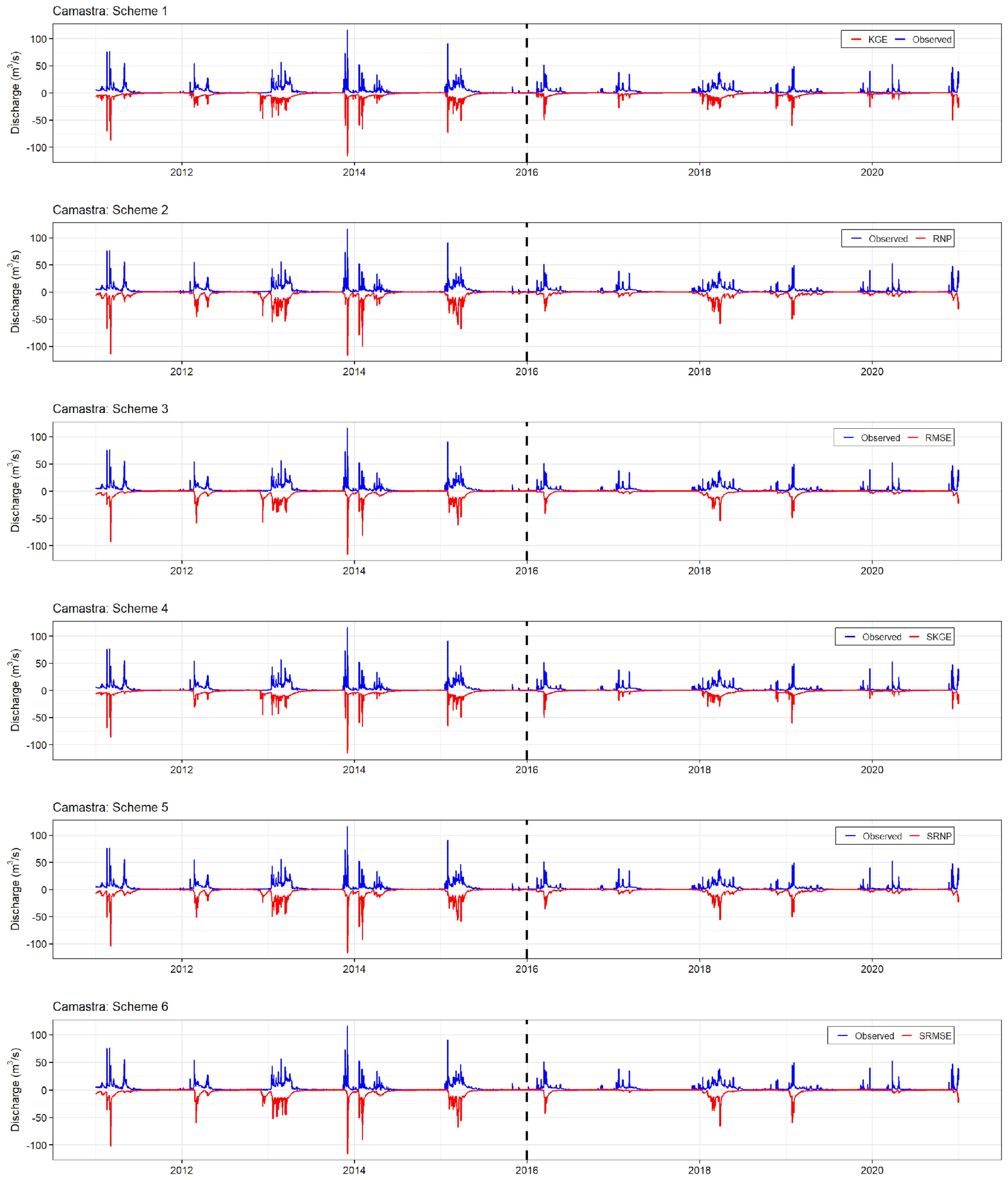
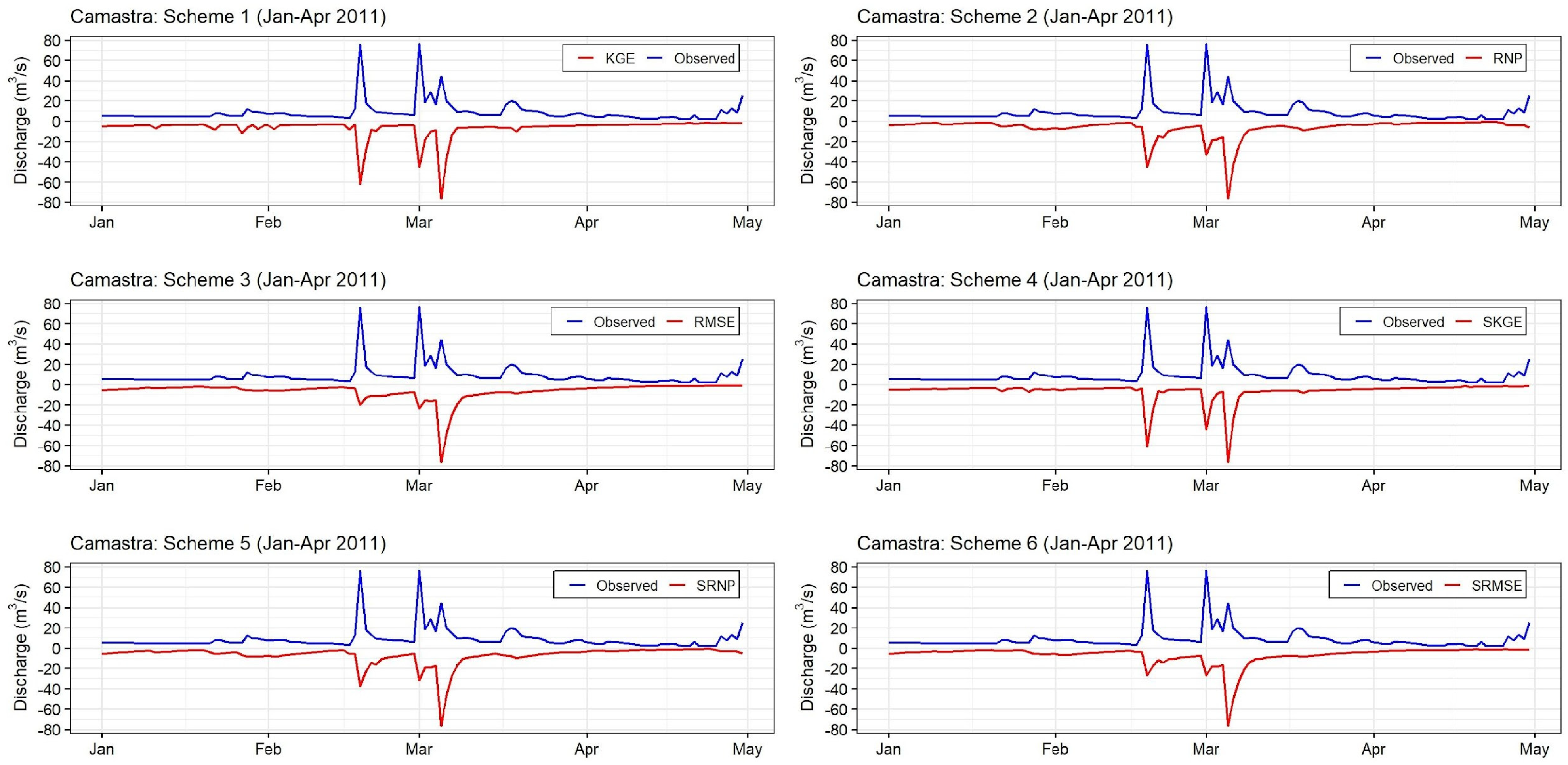
Comparing the strategies, scheme 2 excelled in validation FPR and NSE due to its non-parametric FDC integration (αNP, rs), followed by scheme 1 with superior calibration RMSE via parametric alignment and scheme 3 with minimal calibration PBIAS but weaker validation NSE from distribution-only focus. Time-consistent variants (schemes 4–6) substantially enhanced high-flow transferability (e.g., 10–15% PBIAS reductions, 3–8% FPR improvements), with scheme 5 offering the best balance by curbing DAMN through sub-period rank averaging [23,24,25,26,27,28,29,30,31,32,33,34,35,36,37,38,39,40,41,42,43]. Calibration duration significantly influenced outcomes: longer periods (e.g., Camastra/Ofanto, 5 years) yielded 10–15% FPR reductions for variants versus 3–5% in shorter ones (e.g., Alaco, 2 years), emphasizing sufficient data for peak variability capture. In regulated catchments, scheme 5 mitigated uncertainties better than scheme 1 via reduced outlier sensitivity, supporting robust flood management. Overall, scheme 5 emerges as the most effective for high-flow prediction (10% FPR gain over scheme 2), providing actionable insights for early warning in extreme-prone catchments, with variants enhancing reliability by constraining peak parameters against equifinality. Figure 4 shows the high-flow performance for a sample catchment (Camastra), with scatter plots for all nine study catchments in Supplementary S6.

3.2.2. Analysis of Streamflow FDC Quantiles

FDC matching performance was evaluated using Absolute Percentage Bias (APB = |(Qsim − Qobs)/Qobs| × 100) across five quantiles (Q5, Q25, Q50, Q75, Q95), measuring the deviation of simulated from observed flow durations to assess how well each strategy reproduces the statistical distribution of flows critical for water resource planning in the study area. Table 7 presents the mean ± standard deviation of APB across the nine study catchments for the three calibration strategies and their time-consistent variants during calibration and validation periods, derived from absolute percentage differences and quantile values.
Scheme 1 exhibited moderate calibration APB for Q5 (99.31), decreasing to lower biases in medium flows (Q50: 24.21) but higher in low flows (Q95: 19.35), reflecting KGE’s emphasis on correlation and variability, which aligns high-flow magnitudes by optimizing TUW’s fast-routing parameters (K0, K1) against peak variances but struggles with low-flow tails due to parametric least-squares favoring high-magnitude residuals over tail equity. However, it achieved the lowest validation APB for Q5 (51.63%), Q25 (38.91%), and Q75 (14.95%), as its parametric decomposition into correlation, variability, and bias components promotes temporal dynamics that generalize well beyond the calibration period, mitigating non-stationarity effects in validation data. This transferability stems from KGE’s ability to balance overall hydrograph fit through β-bias correction, which embeds process insights (e.g., soil storage FC for mid-flow persistence) for robust extrapolation in bimodal regimes, making it less prone to overfitting distribution-specific artifacts in data-scarce settings. Validation APB decreased for Q5 (51.63), with PBIAS indicating underestimation in extremes. The time-consistent variant, scheme 4, reduced calibration APB for Q5 (89.86) and validation for Q95 (36.07) by averaging KGE over sub-periods, improving transferability, particularly in catchments with longer durations (e.g., 5 years for Ofanto, APB reduction ~15% for Q50). Scheme 4′s sub-period averaging mitigated the DAMN effect, achieving a 10% reduction in validation APB for Q95 (from 24.12 to 22.59) in catchments like Camastra, enhancing low-flow distribution accuracy critical for drought management, by stabilizing low-variability parameters (e.g., K2 for baseflow) across interannual dry spells.
Scheme 2 achieved lower calibration APB for Q5 (105.86), Q25 (68.90), and Q95 (20.92), leveraging non-parametric αNP (normalized FDC) and rs to capture the full flow spectrum without normality assumptions, resulting in balanced distribution matching. Notably, it delivered the lowest calibration APB for Q75 (10.88%), owing to its ranked correlation (rs) and FDC-derived variability (αNP), which equitably weight mid-range flows without the high-flow dominance of parametric metrics like KGE, thus better suiting the skewed, intermittent regimes of our catchments. This hybrid approach yielded superior low-flow performance, as αNP directly uses ranked flows to reduce bias in tails. Validation APB for Q5 (94.39) remained relatively high but demonstrated robustness to non-stationarity hydrologic regime. The time-consistent variant, scheme 5, improved validation APB for Q75 (22.47) and Q95 (20.01) through sub-period averaging to address DAMN and amalgamation effects, with greater benefits in extended periods (e.g., 5 years for Basento, Q50 APB decrease ~12%). Scheme 5 excelled with the lowest APB for Q95 in both calibration (18.67%) and validation (20.01%) and for Q50 in validation (24.87%) because its non-parametric structure-combining Spearman rank correlation and normalized FDC components avoid assumptions of linearity and normality, while sub-period averaging enforces consistency across interannual variability, reducing equifinality and enhancing low- to mid-flow stability in non-stationary environments. This is particularly advantageous for the study catchments, where low flows are sensitive to prolonged dry spells and reconstructed records.
Scheme 3 minimized calibration APB for Q5 (59.01), Q25 (21.73), Q50 (13.13) and Q95 (5.41), as RMSErank’s magnitude-focused optimization directly targets distribution, excelling in medium and low flows but showing higher bias in extremes due to lack of temporal correlation. It dominated calibration performance across Q5, Q25, and Q50 (lowest APBs of 59.01%, 21.73%, and 13.13%, respectively), justified by its explicit minimization of errors on sorted flow magnitudes, which inherently prioritizes quantile matching over temporal sequencing, ideal for capturing the statistical essence of ephemeral, bimodal Mediterranean flows during the fitting phase without high-flow bias [34,36]. Validation APB for Q95 (13.91) was competitive, highlighting suitability for signature-based applications in data-scarce settings. The time-consistent variant, scheme 6, lowered calibration APB for Q5 (79.98) and validation for Q25 (85.99) via sub-period FDC averaging, alleviating biases in shorter durations (e.g., 2 years for Alaco, Q75 reduction ~7%), though higher SD in low flows (Q95: 23.66) indicates sensitivity to period length, as annual averaging constrains tail biases less effectively without temporal anchors.
A key feature of this study is the reconstruction of inflow discharge for the five regulated reservoirs due to the lack of direct measurements. These reconstructions used water balance equations, including daily storage changes, outflows, and evaporation from the lake surface via the Blaney–Criddle method, which estimates evapotranspiration from temperature and daylight but ignores humidity and wind speed, yielding uncertainty in Mediterranean summers [101,102]. Errors in storage gauging or unmonitored inflows bias estimates, often understating low flows or overstating peaks.
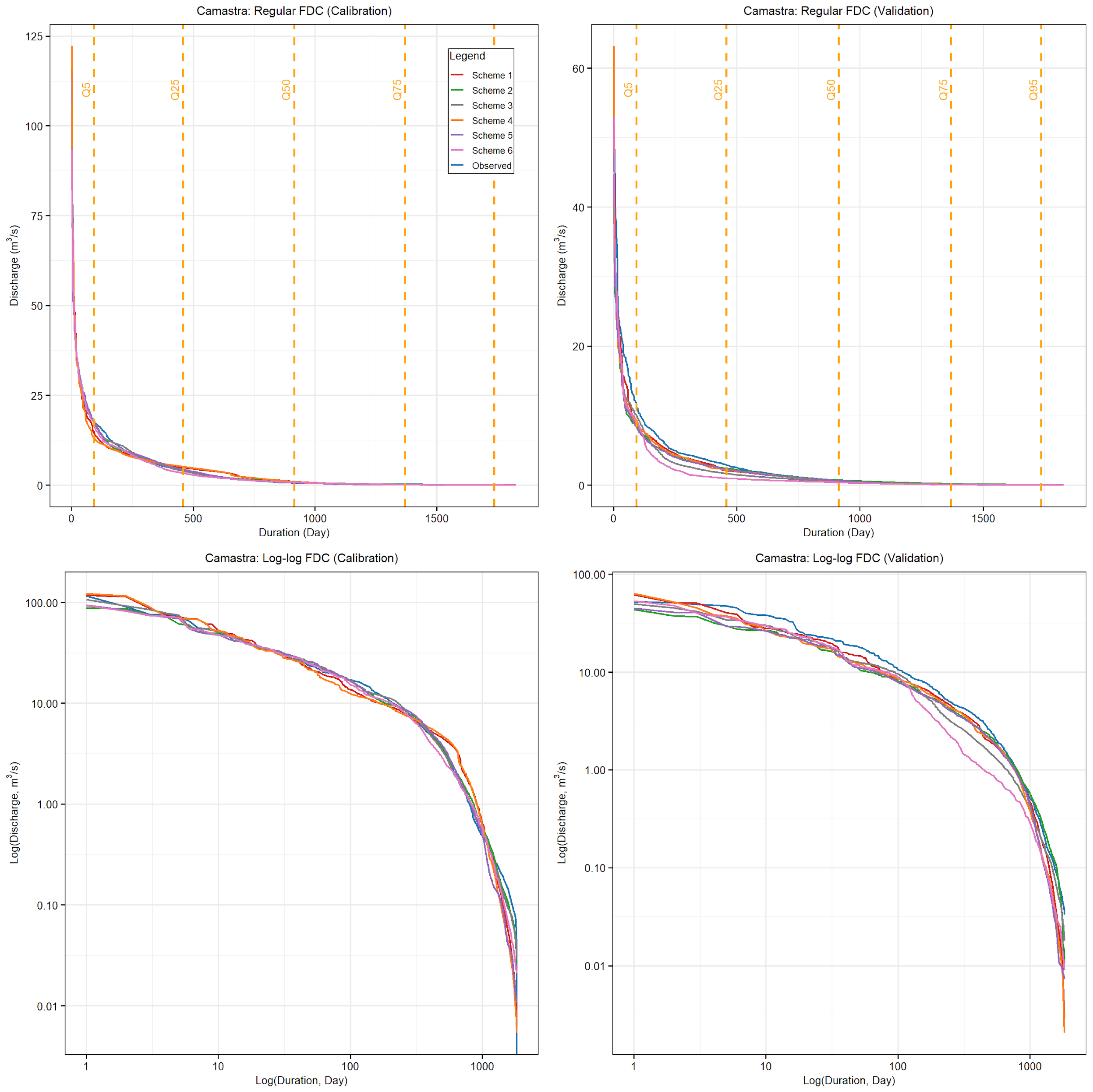
Such uncertainties affect strategies variably, especially FDC-based calibration (scheme 3). Hydrograph metrics (e.g., KGE, RNP) temper errors via temporal penalties and correlations, but FDC’s focus on quantiles (Q5–Q95) heightens vulnerability to low-flow distortions. For example, underestimated evaporation may inflate baseflows, distorting FDCs toward persistence and biasing parameters like k2 (slower recessions), explaining strong calibration (low APB in Q95; Table 7) but weak validation (high biases in reservoirs; Figure 5). This echoes signature methods’ input sensitivity in ephemeral flows, where data gaps worsen low-flow equifinality.
Notably, base schemes (1–3) generally outperformed their time-consistent counterparts (4–6) across most quantiles in both calibration and validation—except for Q50 in validation—because the former optimize over full-period time series or distributions, capturing overarching trends and reducing aggregation-induced smoothing of interannual signals, whereas the latter average objectives over shorter sub-periods, which can amplify noise from variable annual conditions (e.g., isolated dry years) and introduce higher variability in quantile estimates, particularly in data-scarce contexts with limited sub-period length. This full-period advantage holds despite time-consistent variants’ intended mitigation of DAMN, as the averaging dilutes extreme quantile fidelity in non-stationary regimes unless sub-periods are sufficiently long and representative.
These findings underscore a strategic interplay between calibration fidelity and validation robustness, emblematic of the trade-offs in objective function design for non-stationary hydrological modeling. Scheme 3′s calibration supremacy in high- and mid-flow quantiles (Q5–Q50) validates the efficacy of signature-based approaches in distilling catchment behavior from sparse data, making it optimal for distribution-focused tasks requiring precise reproduction of flow regimes within the fitting period (direct RMSErank penalization of sorted errors). Conversely, scheme 1′s validation edge in Q5, Q25, and Q75 reflects the parametric robustness of KGE, which embeds hydrological process insights (e.g., via bias and variability ratios) to foster temporal extrapolation, though at the cost of low-flow underrepresentation—a common critique in drying climate due to r’s sensitivity to peak timing mismatch. Meanwhile, scheme 2 excelled in calibration low flows owing to non-parametric FDC integration, while the standout performance of scheme 5 across low-flow (Q95) and validation median (Q50) quantiles highlights time-consistent non-parametric calibration as a paradigm shift: by averaging over annual sub-periods, it curtails the DAMN effect [43] and equifinality, yielding parameters that are not only stable but ecologically relevant for drought-prone Mediterranean systems (e.g., supporting baseflow indices for water allocation) through rank-stable optimization of recession (BMAX). Overall, these patterns advocate hybrid strategies—pairing FDC for initial distribution tuning with SRNP for operational generalization—offering a pathway to resilient modeling amid climate variability and monitoring gaps in southern Italy, thus underscoring the strategic advantage of tailored calibration approaches in data-scarce settings.
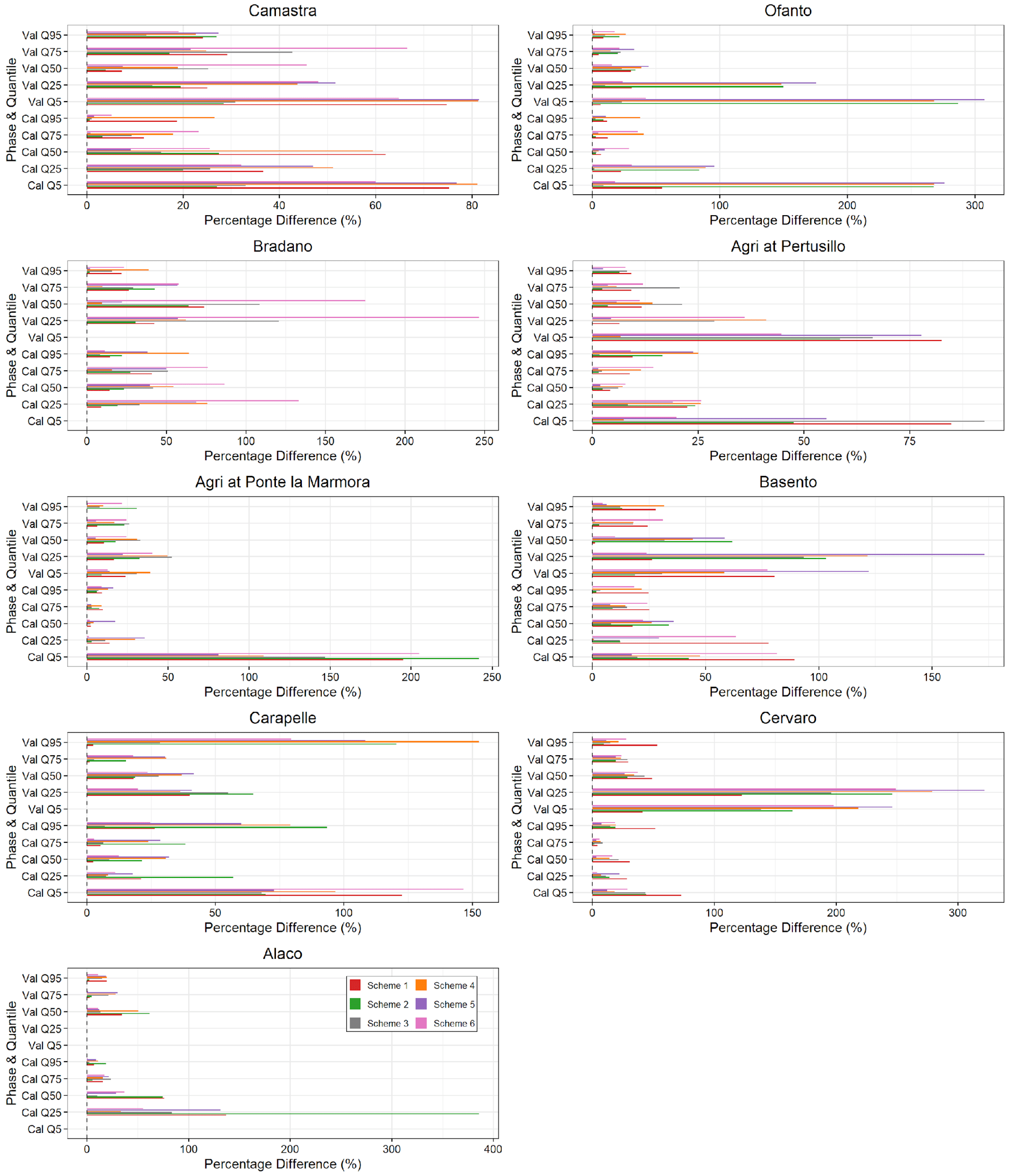
Figure 5 illustrates the FDC matching performance for the Camastra catchment, comparing log-log and linear-scale FDCs across calibration schemes. Figure 6 reports the percentage differences between simulated and observed FDC quantiles for all six schemes, while Supplementary S7 provides the corresponding FDCs for all study catchments.

3.3. Model Parameters Variability

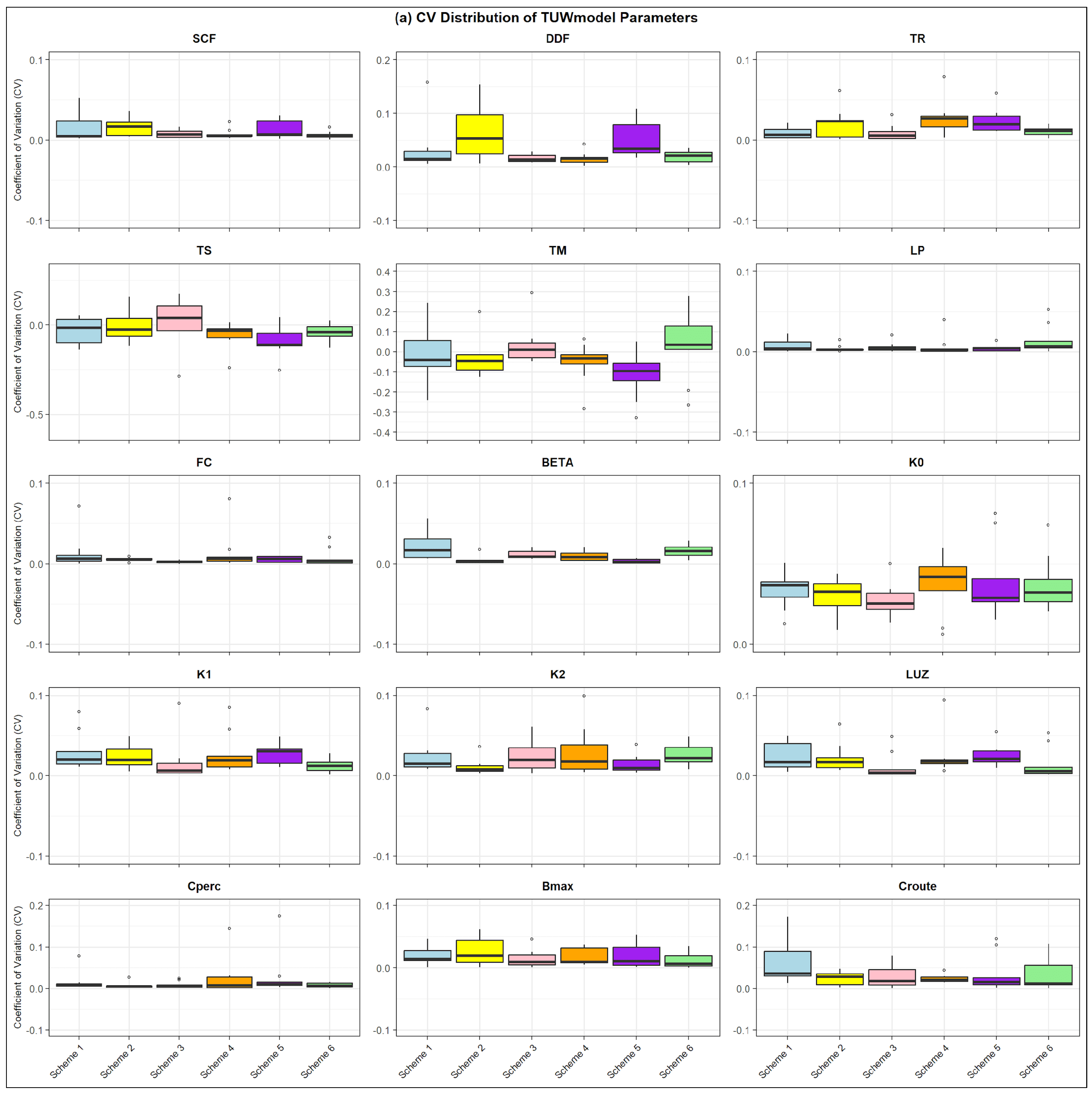
Parameter stability represents a critical indicator of model reliability and transferability, particularly in data-scarce environments where equifinality—the existence of multiple parameter sets producing similar performance—undermines predictive confidence [17,103]. To quantify parameter stability across calibration strategies, we analyzed the coefficient of variation (CV) of the 15 model parameters using the top-performing parameter sets (n = 100) from the GA optimization. This is an efficient method that was used to understand how big (or small) parameter uncertainty is for the very best values of each function. Here, lower CV values indicate greater parameter consistency and reduced equifinality, suggesting more reliable parameter identification [104]. Figure 7 displays the boxplots of the 15 model parameters for all calibration strategies and their corresponding time-consistent variants.
Scheme 1 exhibited a mean CV of 0.01 across all parameters, with moderate variability in K0 (0.037), indicating some sensitivity in very fast flow due to its focus on overall hydrograph correlation, variability, and bias (see Table 8) [47]. Parameters like SCF (0.005) and BMAX (0.014) showed very low CV, indicating high stability in snow correction and baseflow recession processes. Scheme 4 maintained a mean CV of 0.017, with minor reductions in LP (0.002 from 0.005) and Croute (0.023 from 0.036), as sub-period averaging enforces consistent performance across annual sub-periods, narrowing the parameter space and reducing equifinality by 2–5% for key parameters [104].
Scheme 2 had a mean CV of 0.011, with low variability in BETA (0.003) and Cperc (0.005), reflecting its non-parametric FDC focus (αNP) that constrains flexibility in flux parameters while maintaining very low CV in routing (K2: 0.008). This balance makes scheme 2 effective for catchments with skewed flow regimes, such as Alaco, where non-parametric metrics reduce sensitivity to reconstructed inflow errors. Scheme 5 presented a mean CV of 0.023 ± 0.03, with a slight increase in variability in K2 (from 0.008 to 0.010) yet minimal dispersion in Cperc (from 0.005 to 0.011), indicative of subtle trade-offs in percolation dynamics under sub-period non-parametric assessment—mirroring observations in literature where multivariate calibration can modestly amplify equifinality in certain parameter dimensions [14].
Scheme 3 (FDC-based) manifested a mean CV of 0.012, with low variability in TS (0.048) and TM (0.01), as the RMSErank optimization, centered on flow magnitude distribution, moderates uncertainty in snow routine parameters. Scheme 6 (SRMSE) attained a mean CV of −0.00, featuring notable reductions in TS (from 0.048 to −0.052) and BMAX (from 0.010 to 0.007), demonstrating that sub-period FDC matching effectively constrains the parameter space by 3–8%, thereby bolstering transferability amid non-stationary hydrologic regimes—a strategy akin to hydrograph separation techniques that sequentially calibrate flow components to curtail equifinality [105].
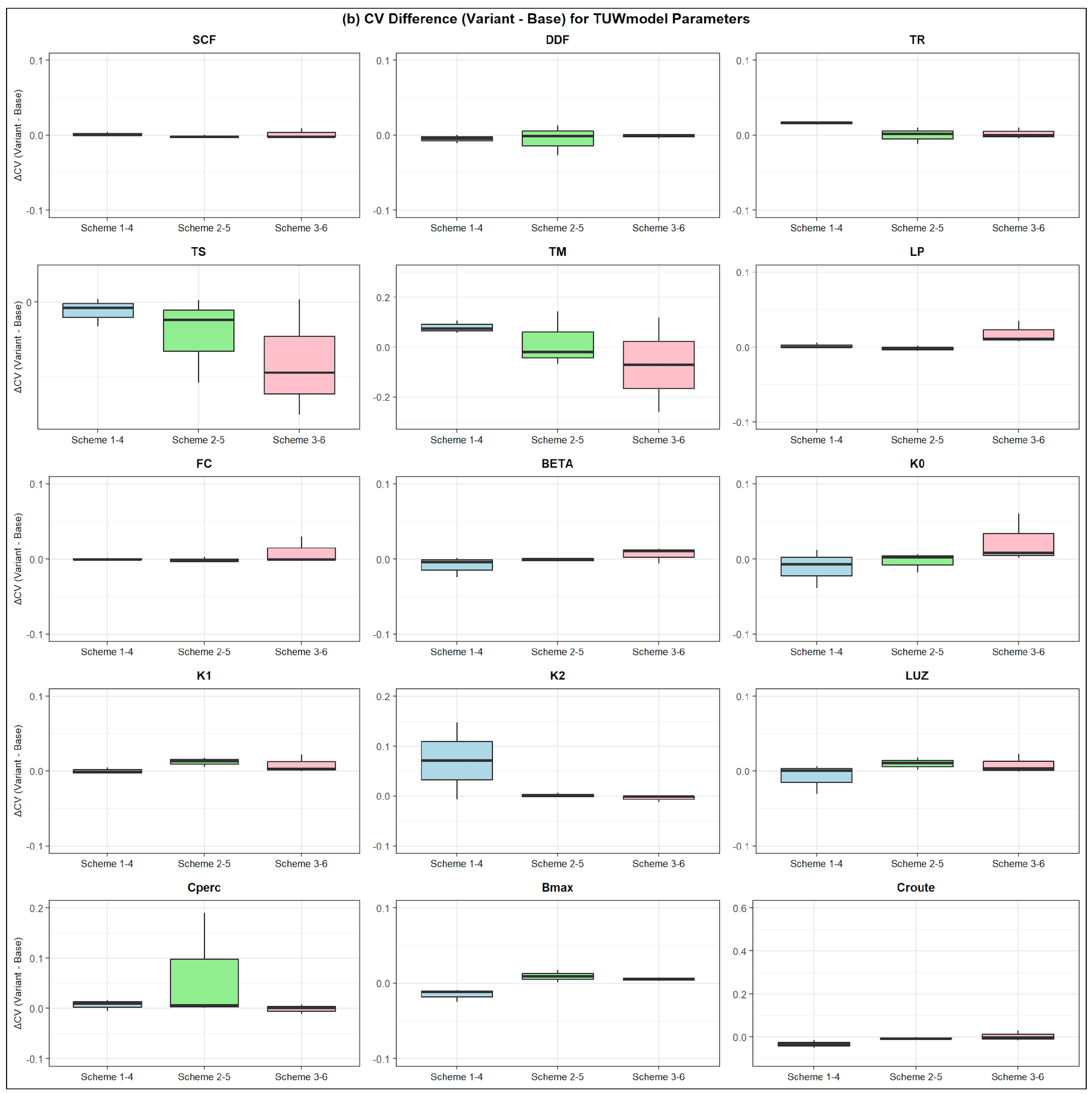
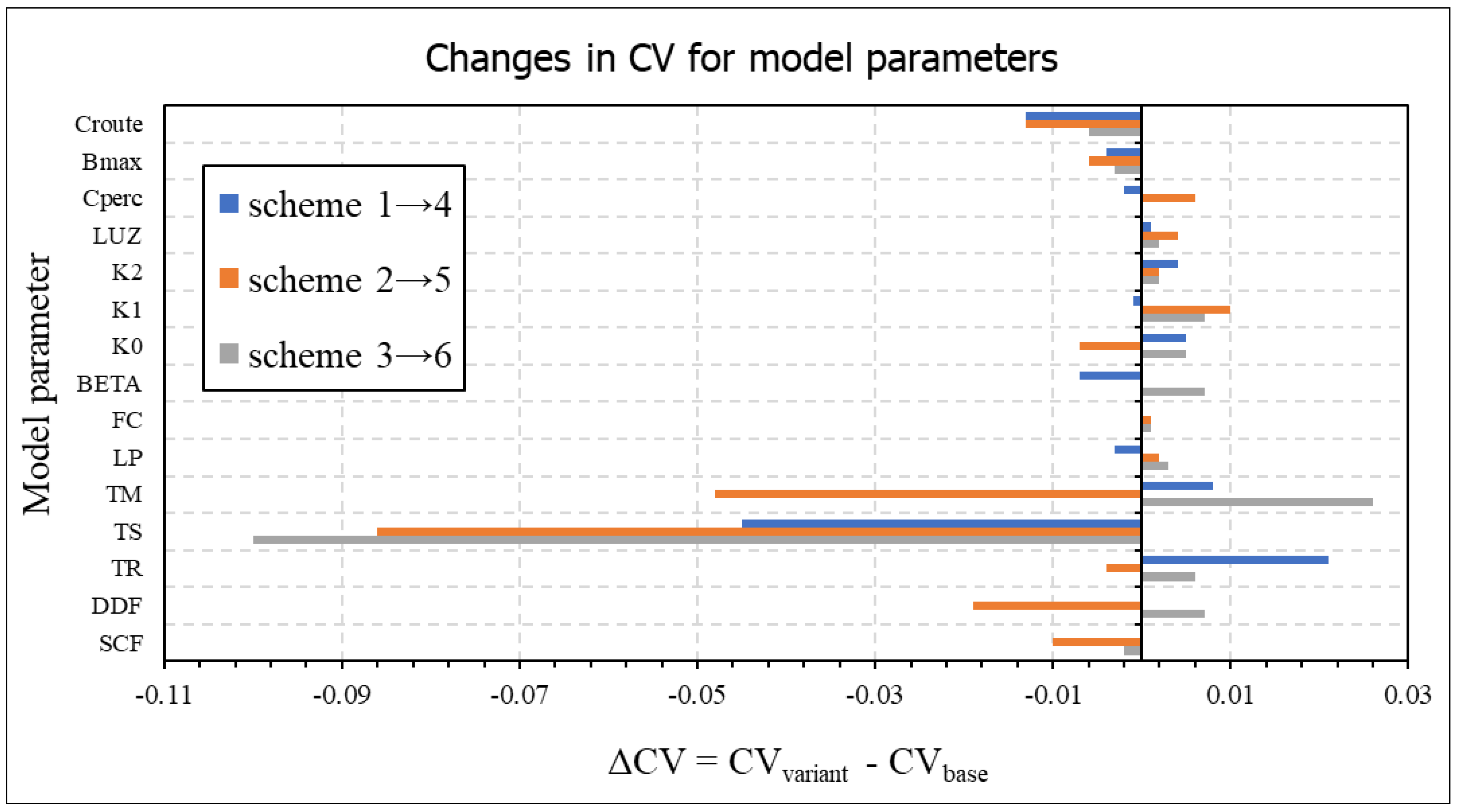
To further elucidate the impact of time-consistent calibration on parameter stability, we computed pairwise differences in median CVs (ΔCV = CVvariant − CVbase) between base schemes (1–3) and their variants (4–6), as summarized in Figure 7b and Figure 8. Across all 15 parameters and pairs, negative ΔCVs predominated over positives, with four zeros, yielding net stability gains that underscore the variants’ efficacy in constraining the parameter space and mitigating equifinality under non-stationary hydrologic conditions [23]. Notably, snow-related parameters exhibited consistent reductions, with TS showing the largest gains (ΔCV: −0.045 for SKGE, −0.086 for SRNP, −0.100 for SRMSE), reflecting sub-period averaging’s ability to better resolve threshold uncertainties in the study catchments with variable winter regimes. Routing parameters like Croute also benefited uniformly (ΔCV: −0.013 to −0.006), enhancing baseflow transferability, while soil storage (FC) remained largely stable (near-zero Δs). Trade-offs emerged in melt (TM) and fast-flow (K0) dynamics, particularly for the FDC→SRMSE pair (positive ΔCVs of +0.026 and +0.005, respectively), where magnitude-focused optimization amplified sub-period sensitivities. The SRNP variant (scheme 5) demonstrated the strongest overall reductions (mean ΔCV = −0.008), balancing non-parametric robustness with temporal consistency, whereas SKGE (scheme 4) and SRMSE (scheme 6) showed more balanced but slightly mixed outcomes (means −0.002 and +0.002). These patterns affirm time-consistent approaches’ value in data-scarce settings, though scheme selection should prioritize hydrological context to minimize isolated losses in process-specific parameters.
An examination of parameter-specific variability unveils consistent patterns across schemes. Low CV values were evident for LUZ (mean 0.013), signifying limited uncertainty in upper zone thresholds, attributable to their pivotal role in fast runoff mechanisms less susceptible to high-flow biases in calibration [106]. Likewise, CPERC (mean 0.007) displayed low variability, encapsulating fewer challenges in modeling percolation under varied objective functions [107]. Conversely, very subdued CV was observed for SCF (mean 0.007) and TR (mean 0.015), implying high robustness in snow correction and precipitation partitioning parameters, minimally influenced by temporal segmentation [106]. Routing parameters, including K0 (mean 0.033) and K2 (mean 0.015), exhibited low variability, equilibrating baseflow fidelity across strategies [3,47,105]. These patterns resonate with flux-mapping approaches that advocate for internal consistency checks to discern behavioral parameter sets amid equifinality [58].
In comparative terms, schemes 4 and 5 attained the lowest mean CV, evincing paramount parameter stability for magnitude-oriented calibration, followed by schemes 1 and 6 with high stability for hydrograph-oriented calibration, and succeeded by scheme 2 with balanced variability for non-parametric distribution matching, while scheme 5 (0.023) registered the highest due to its sub-period non-parametric optimization. Time-consistent variants (schemes 4, 5, and 6) generally attenuated CV for salient parameters (e.g., SCF, K0, BMAX, Croute) by 2–8%, with scheme 6 offering optimal equilibrium at a mean CV of 0.009, effectively curbing equifinality in routing and storage domains across catchments. This corroborates broader literature emphasizing that incorporating additional constraints, such as multi-parameter ensembles or process-based separations, substantially mitigates uncertainty in climate-impacted hydrological projections, where parameter equifinality often rivals or exceeds General Circulation Model-derived variability [106,107].
Yet, multi-metric evaluation and time-consistent variants (schemes 4–6) alleviate propagation through hydrograph cross-checks (e.g., NSE) and sub-period stability, showing solid FDC results in natural catchments (ΔAPB < 5%) over reservoirs. Future work should add uncertainty quantification (e.g., Monte Carlo for evaporation) or remote sensing lake levels to bolster FDC for regulated catchment forecasting.

4. Conclusions

This study presents a comprehensive comparison of three calibration strategies—KGE-based (scheme 1), non-parametric RNP-based (scheme 2), and FDC-based (scheme 3)—along with their three time-consistent variants (SKGE [scheme 4], SRNP [scheme 5], and SRMSE [scheme 6]). These were applied to the lumped HBV-based TUW model across nine data-scarce catchments in southern Italy. This analysis addresses the issues arising from non-stationary streamflow regimes and systematic data errors. While the time-consistent KGE-based strategy demonstrated good calibration performance through its parametric decomposition of correlation, variability, and bias, a notable decline in validation performance underscores its sensitivity to non-stationarity and data limitations, suggesting potential overfitting of the calibration. The RNP-based strategy exhibited superior robustness in validation, maintaining an effective balance across flow regimes, particularly with regard to low-flow accuracy, due to its non-parametric structure leveraging rank-based FDC normalization and Spearman correlation. The FDC-based strategy excelled in calibration by achieving the lowest PBIAS, effectively reproducing the statistical distribution of flows, but its limited temporal transferability was evident with increased validation biases, from neglecting hydrograph sequencing.
The application of time-consistent variants, where objective functions were averaged over individual years, markedly enhanced model reliability across all catchments. These variants improved validation performance, with SKGE, SRNP, and SRMSE contributing to greater robustness to non-stationary streamflow regimes. Parameter stability was also significantly bolstered by time-consistent variants, reducing equifinality and improving model transferability through sub-period averaging. The results reveal a clear trade-off between calibration accuracy and validation robustness, influenced by the choice of objective function. While the KGE-based approach excels in calibration, its validation limitations suggest it is less suited for long-term predictions in data-scarce settings. Conversely, RNP-based approaches and time-consistent variants offer a more balanced performance, with the latter proving critical for non-stationary streamflow regimes of Mediterranean environments. The SRNP variant emerges as the most balanced approach for generalization, balancing quantile matching with temporal equity, recommending its adoption for enhanced reliability. The use of time-consistent variants for calibration, particularly SRNP and SRMSE, is recommended to improve model performance, with potential benefits when applied to extended calibration periods. Future research should explore the integration of additional hydrological signatures (e.g., baseflow indices) and adaptive techniques (e.g., Bayesian ensembles) to further address evolving data constraints and climate variability in similar regions.

Supplementary Materials

The following supporting information can be downloaded at: https://www.mdpi.com/article/10.3390/hydrology13020066/s1.

Author Contributions

Conceptualization, A.J. and P.P.; and S.M.; methodology, A.J., P.P. and A.A.; software, A.J. and F.D.P.; validation, A.A., P.P. and A.A.; formal analysis, A.J. and A.N.S.; investigation, A.J., P.P., SM. and R.Z.; resources, U.T.; data curation, P.C. and L.G.; writing—original draft preparation, A.J.; writing—review and editing, A.J., P.P., A.A., F.D.P., A.N.S. and S.M.; visualization, A.J.; supervision, S.M.; project administration, S.M.; funding acquisition, S.M. All authors have read and agreed to the published version of the manuscript.

Funding

This research was funded by financial resources from Next Generation EU and the Italian Ministry of University and Research through the PRIN PNRR 2022 project “An integrated modeling approach for mitigating climate change effects through enhanced weathering in Southern Italy” (CHANCES-CUP E53D23021850001). It also received funding from the RETURN Extended Partnership, under the European Union’s Next Generation EU initiative (National Recovery and Resilience Plan-NRRP, Mission 4, Component 2, Investment 1.3-D.D. 1243 of 2 August 2022, PE0000005). Additional support was provided through a research agreement with the River Basin Authority of Southern Italy, entitled “Development of a Hydrological Budget Model and the Design of a Hydro-Meteorological Monitoring Network for the Southern Apennines District”, funded by the Development and Cohesion Fund 2014–2020 (PED Acque-CUP F52G16000010001). This work was also carried out within the framework of the Programme in Sustainable Development and Climate Change University School for Advanced Studies IUSS Pavia, carried out at University of Naples Federico II–XXXIX Cycle–Funded by the European Union NextgenerationEU-PNRR. Type of scholarship: DM118/2023-M4C1–Inv. 4.1-Pubblica Amministrazione I53C23000820001.

Data Availability Statement

The data used in this study are available from the corresponding author upon request. All datasets were processed and analysed within the framework of the present study.

Acknowledgments

The authors would like to express their sincere gratitude to the River Basin Authority of Southern Apennine (Autorità di Bacino Distrettuale dell’Appennino Meridionale) for kindly providing the essential data that formed the foundation of this study. We are also deeply thankful to the Department of Civil, Architectural and Environmental Engineering (DICEA) of the University of Naples Federico II for their valuable collaboration, technical support, and access to resources throughout the research project. The authors further acknowledge Vera Corbelli for her continuous support of the research activities and for fostering constructive dialogue between the scientific and institutional communities.

Conflicts of Interest

Author Pasquale Perrini was employed by the company Consorzio Interuniversitario per l’Idrologia. The remaining authors declare that the research was conducted in the absence of any commercial or financial relationships that could be construed as a potential conflict of interest.

References

  1. Knoben, W.J.M.; Freer, J.E.; Woods, R.A. Technical Note: Inherent Benchmark or Not? Comparing Nash-Sutcliffe and Kling-Gupta Efficiency Scores. Hydrol. Earth Syst. Sci. 2019, 23, 4323–4331. [Google Scholar] [CrossRef]
  2. Manfreda, S.; Mita, L.; Dal Sasso, S.F.; Samela, C.; Mancusi, L. Exploiting the Use of Physical Information for the Calibration of a Lumped Hydrological Model. Hydrol. Process. 2018, 32, 1420–1433. [Google Scholar] [CrossRef]
  3. Seibert, J.; Vis, M.J.P. Teaching Hydrological Modeling with a User-Friendly Catchment-Runoff-Model Software Package. Hydrol. Earth Syst. Sci. 2012, 16, 3315–3325. [Google Scholar] [CrossRef]
  4. Sheikh, M.R.; Coulibaly, P. Hydrologic Model Calibration Approaches for Highly Regulated River Basin: A Comprehensive Assessment. J. Hydrol. Reg. Stud. 2025, 58, 102198. [Google Scholar] [CrossRef]
  5. Wallner, M.; Haberlandt, U.; Dietrich, J. Evaluation of Different Calibration Strategies for Large Scale Continuous Hydrological Modelling. Adv. Geosci. 2012, 31, 67–74. [Google Scholar] [CrossRef]
  6. Kalura, P.; Pandey, A.; Chowdary, V.M.; Dayal, D. A TOPSIS-Based Multicriteria Assessment of Hydrologic Model Calibration Using Satellite-Derived Evapotranspiration and Streamflow Data. Hydrol. Process. 2025, 39, e70191. [Google Scholar] [CrossRef]
  7. Anand, V.; Oinam, B.; Wieprecht, S.; Singh, S.K.; Srinivasan, R. Enhancing Hydrological Model Calibration through Hybrid Strategies in Data-Scarce Regions. Hydrol. Process. 2024, 38, e15084. [Google Scholar] [CrossRef]
  8. Westerberg, I.K.; Sikorska-Senoner, A.E.; Viviroli, D.; Vis, M.; Seibert, J. Hydrological Model Calibration with Uncertain Discharge Data. Hydrol. Sci. J. 2022, 67, 2441–2456. [Google Scholar] [CrossRef]
  9. Jansen, K.F.; Teuling, A.J.; Craig, J.R.; Dal Molin, M.; Knoben, W.J.M.; Parajka, J.; Vis, M.; Melsen, L.A. Mimicry of a Conceptual Hydrological Model (HBV): What’s in a Name? Water Resour. Res. 2021, 57, e2020WR029143. [Google Scholar] [CrossRef]
  10. Mai, J. Ten Strategies towards Successful Calibration of Environmental Models. J. Hydrol. 2023, 620, 129414. [Google Scholar] [CrossRef]
  11. Guo, X.; Wu, Z.; Fu, G.; He, H. A Multi-Variable Calibration Framework at the Grid Scale for Integrating Streamflow with Evapotranspiration Data to Improve the Simulation of Distributed Hydrological Model. J. Hydrol. Reg. Stud. 2024, 55, 101944. [Google Scholar] [CrossRef]
  12. McMillan, H.; Freer, J.; Pappenberger, F.; Krueger, T.; Clark, M. Impacts of Uncertain River Flow Data on Rainfall-Runoff Model Calibration and Discharge Predictions. Hydrol. Process. 2010, 24, 1270–1284. [Google Scholar] [CrossRef]
  13. Pushpalatha, R.; Perrin, C.; Le Moine, N.; Andréassian, V. A Review of Efficiency Criteria Suitable for Evaluating Low-Flow Simulations. J. Hydrol. 2012, 420–421, 171–182. [Google Scholar] [CrossRef]
  14. Pool, S.; Vis, M.; Seibert, J. Evaluating Model Performance: Towards a Non-Parametric Variant of the Kling-Gupta Efficiency. Hydrol. Sci. J. 2018, 63, 1941–1953. [Google Scholar] [CrossRef]
  15. Beven, K. A Manifesto for the Equifinality Thesis. J. Hydrol. 2006, 320, 18–36. [Google Scholar] [CrossRef]
  16. Schoups, G.; Vrugt, J.A. A Formal Likelihood Function for Parameter and Predictive Inference of Hydrologic Models with Correlated, Heteroscedastic, and Non-Gaussian Errors. Water Resour. Res. 2010, 46, 10. [Google Scholar] [CrossRef]
  17. Beven, K. Prophecy, Reality and Uncertainty in Distributed Hydrological Modelling. Adv. Water Resour. 1993, 16, 41–51. [Google Scholar] [CrossRef]
  18. Brigode, P.; Oudin, L.; Perrin, C. Hydrological Model Parameter Instability: A Source of Additional Uncertainty in Estimating the Hydrological Impacts of Climate Change? J. Hydrol. 2013, 476, 410–425. [Google Scholar] [CrossRef]
  19. Fowler, K.J.A.; Peel, M.C.; Western, A.W.; Zhang, L.; Peterson, T.J. Simulating Runoff under Changing Climatic Conditions: Revisiting an Apparent Deficiency of Conceptual Rainfall-Runoff Models. Water Resour. Res. 2016, 52, 1820–1846. [Google Scholar] [CrossRef]
  20. Freer, J.; Beven, K.; Ambroise, B. Bayesian Estimation of Uncertainty in Runoff Prediction and the Value of Data: An Application of the GLUE Approach. Water Resour. Res. 1996, 32, 2161–2173. [Google Scholar] [CrossRef]
  21. Krause, P.; Boyle, D.P.; Bäse, F. Comparison of Different Efficiency Criteria for Hydrological Model Assessment. Adv. Geosci. 2005, 5, 89–97. [Google Scholar] [CrossRef]
  22. Berthet, L.; Andréassian, V.; Perrin, C.; Loumagne, C. Quelle Signification Accorder Aux Critères Quadratiques? Partie 1. Combien d’années Sont Nécessaires Pour Que La Valeur d’un Critère Quadratique Soit Indépendante Des Données? Hydrol. Sci. J. 2010, 55, 1051–1062. [Google Scholar] [CrossRef][Green Version]
  23. Gharari, S.; Hrachowitz, M.; Fenicia, F.; Savenije, H.H.G. An Approach to Identify Time Consistent Model Parameters: Sub-Period Calibration. Hydrol. Earth Syst. Sci. 2013, 17, 149–161. [Google Scholar] [CrossRef]
  24. Li, C.Z.; Zhang, L.; Wang, H.; Zhang, Y.Q.; Yu, F.L.; Yan, D.H. The Transferability of Hydrological Models under Nonstationary Climatic Conditions. Hydrol. Earth Syst. Sci. 2012, 16, 1239–1254. [Google Scholar] [CrossRef]
  25. Nearing, G.S.; Gupta, H.V. The Quantity and Quality of Information in Hydrologic Models. Water Resour. Res. 2015, 51, 524–538. [Google Scholar] [CrossRef]
  26. Santos, L.; Thirel, G.; Perrin, C. Technical Note: Pitfalls in Using Log-Transformed Flows within the KGE Criterion. Hydrol. Earth Syst. Sci. 2018, 22, 4583–4591. [Google Scholar] [CrossRef]
  27. Moriasi, D.N.; Arnold, J.G.; van Liew, M.W.; Bingner, R.L.; Harmel, R.D.; Veith, T.L. Model Evaluation Guidelines for Systematic Quantification of Accuracy in Watershed Simulations. Trans. ASABE 2007, 50, 885–900. [Google Scholar] [CrossRef]
  28. Montanari, A.; Di Baldassarre, G. Data Errors and Hydrological Modelling: The Role of Model Structure to Propagate Observation Uncertainty. Adv. Water Resour. 2013, 51, 498–504. [Google Scholar] [CrossRef]
  29. Estrada, L.; Garcia, X.; Saló-Grau, J.; Marcé, R.; Munné, A.; Acuña, V. Spatio-Temporal Patterns and Trends of Streamflow in Water-Scarce Mediterranean Basins. Hydrol. Earth Syst. Sci. 2024, 28, 5353–5373. [Google Scholar] [CrossRef]
  30. Erol, A.; Randhir, T.O. Climatic Change Impacts on the Ecohydrology of Mediterranean Watersheds. Clim. Change 2012, 114, 319–341. [Google Scholar] [CrossRef]
  31. Yokoo, Y.; Sivapalan, M. Towards Reconstruction of the Flow Duration Curve: Development of a Conceptual Framework with a Physical Basis. Hydrol. Earth Syst. Sci. 2011, 15, 2805–2819. [Google Scholar] [CrossRef]
  32. Vogel, R.M.; Fennessey, N.M. Flow-Duration Curves. I: New Interpretation and Confidence Intervals. J. Water Resour. Plan. Manag. 1994, 120, 485–504. [Google Scholar] [CrossRef]
  33. Manfreda, S.; Fiorentino, M.; Icobellis, V. DREAM: A Distributed Model for Runoff, Evapotranspiration, and Antecedent Soil Moisture Simulation. Adv. Geosci. 2005, 2, 31–39. [Google Scholar] [CrossRef]
  34. Westerberg, I.K.; Guerrero, J.; Younger, P.; Beven, K.J.; Seibert, J.; Halldin, S.; Freer, J.E.; Xu, C. Calibration of Hydrological Models Using Flow-Duration Curves. Hydrol. Earth Syst. Sci. 2011, 15, 2205–2227. [Google Scholar] [CrossRef]
  35. Sahraei, S.; Asadzadeh, M.; Unduche, F. Signature-Based Multi-Modelling and Multi-Objective Calibration of Hydrologic Models: Application in Flood Forecasting for Canadian Prairies. J. Hydrol. 2020, 588, 125095. [Google Scholar] [CrossRef]
  36. Shafii, M.; Tolson, B.A. Optimizing Hydrological Consistency by Incorporating Hydrological Signatures into Model Calibration Objectives. Water Resour. Res. 2015, 51, 3796–3814. [Google Scholar] [CrossRef]
  37. Melišová, E.; Vizina, A.; Staponites, L.R.; Hanel, M. The Role of Hydrological Signatures in Calibration of Conceptual Hydrological Model. Water 2020, 12, 3401. [Google Scholar] [CrossRef]
  38. Truyen Huynh, N.N.; Garambois, P.-A.; Colleoni, F.; Javelle, P. Signatures-and-Sensitivity-Based Multi-Criteria Variational Calibration for Distributed Hydrological Modeling Applied to Mediterranean Floods. J. Hydrol. 2023, 625, 129992. [Google Scholar] [CrossRef]
  39. Kavetski, D.; Fenicia, F.; Reichert, P.; Albert, C. Signature-Domain Calibration of Hydrological Models Using Approximate Bayesian Computation: Theory and Comparison to Existing Applications. Water Resour. Res. 2018, 54, 4059–4083. [Google Scholar] [CrossRef]
  40. Fenicia, F.; Kavetski, D.; Reichert, P.; Albert, C. Signature-Domain Calibration of Hydrological Models Using Approximate Bayesian Computation: Empirical Analysis of Fundamental Properties. Water Resour. Res. 2018, 54, 3958–3987. [Google Scholar] [CrossRef]
  41. Bouizrou, I.; Castelli, G.; Cabrera, G.A.; Villani, L.; Solomos, S.; Maneas, G.; Pantazis, C.; Bresci, E. The Potential of Novel Remote Sensing Evapotranspiration Data and Global Soil Maps for SWAT+ Agro-Hydrological Modeling in Data-Scarce Regions of the North Mediterranean. Agric. Water Manag. 2025, 319, 109761. [Google Scholar] [CrossRef]
  42. Tran Tuan, T. Multiple Conceptual Hydrological Models for Simulating Streamflow in Data-Sparse River Basins: An Application of the Vietnamese Cau River Basin. Water Pract. Technol. 2024, 19, 2944–2958. [Google Scholar] [CrossRef]
  43. Klotz, D.; Gauch, M.; Kratzert, F.; Nearing, G.; Zscheischler, J. Technical Note: The Divide and Measure Nonconformity—How Metrics Can Mislead When We Evaluate on Different Data Partitions. Hydrol. Earth Syst. Sci. 2024, 28, 3665–3673. [Google Scholar] [CrossRef]
  44. Fowler, K.; Peel, M.; Western, A.; Zhang, L. Improved Rainfall-Runoff Calibration for Drying Climate: Choice of Objective Function. Water Resour. Res. 2018, 54, 3392–3408. [Google Scholar] [CrossRef]
  45. Perrini, P.; Iacobellis, V.; Gioia, A.; Cea, L.; Savenije, H.H.G.; Fenicia, F. Can Dominant Runoff Generation Mechanisms Be Disentangled Through Hypothesis Testing? Insights From Integrated Hydrological-Hydrodynamic Modeling. Water Resour. Res. 2025, 61, e2024WR039394. [Google Scholar] [CrossRef]
  46. Boyle, D.P.; Gupta, H.V.; Sorooshian, S. Toward Improved Calibration of Hydrologic Models: Combining the Strengths of Manual and Automatic Methods. Water Resour. Res. 2000, 36, 3663–3674. [Google Scholar] [CrossRef]
  47. Wagener, T.; Boyle, D.P.; Lees, M.; Wheater, H.; Gupta, H.V.; Sorooshian, S. A Framework for Development and Application of Hydrological Models. Water Resour. Res. 2001, 5, 13–26. [Google Scholar] [CrossRef]
  48. Blazkova, S.; Beven, K. A Limits of Acceptability Approach to Model Evaluation and Uncertainty Estimation in Flood Frequency Estimation by Continuous Simulation: Skalka Catchment, Czech Republic. Water Resour. Res. 2009, 45, W00B16. [Google Scholar] [CrossRef]
  49. Han, X.; Yuan, H. Impacts of Precipitation Uncertainty on Hydrological Ensemble Simulations over the Ganjiang River Basin. J. Hydrol. Reg. Stud. 2024, 51, 101617. [Google Scholar] [CrossRef]
  50. Yeste, P.; Melsen, L.A.; García-Valdecasas Ojeda, M.; Gámiz-Fortis, S.R.; Castro-Díez, Y.; Esteban-Parra, M.J. A Pareto-Based Sensitivity Analysis and Multiobjective Calibration Approach for Integrating Streamflow and Evaporation Data. Water Resour. Res. 2023, 59, e2022WR033235. [Google Scholar] [CrossRef]
  51. Global Runoff Data Centre (GRDC). Annual Report 2020; Federal Institute of Hydrology: Koblenz, Germany, 2020. [Google Scholar]
  52. Tramblay, Y.; Rutkowska, A.; Sauquet, E. Trends in Flow Intermittence for European Rivers. Hydrol. Sci. J. 2021, 66, 37–49. [Google Scholar] [CrossRef]
  53. Perrini, P.; Cea, L.; Chiaravalloti, F.; Gabriele, S.; Manfreda, S.; Fiorentino, M.; Gioia, A.; Iacobellis, V. A Runoff-On-Grid Approach to Embed Hydrological Processes in Shallow Water Models. Water Resour. Res. 2024, 60, e2023WR036421. [Google Scholar] [CrossRef]
  54. Gigante, V.; Iacobellis, V.; Manfreda, S.; Milella, P.; Portoghese, I. Influences of Leaf Area Index Estimations on Water Balance Modeling in a Mediterranean Semi-Arid Basin. Nat. Hazards Earth Syst. Sci. 2009, 9, 979–991. [Google Scholar] [CrossRef]
  55. Cammalleri, C.; Naeem Sarwar, A.; Avino, A.; Nikravesh, G.; Bonaccorso, B.; Mendicino, G.; Senatore, A.; Manfreda, S. Testing Trends in Gridded Rainfall Datasets at Relevant Hydrological Scales: A Comparative Study with Regional Ground Observations in Southern Italy. J. Hydrol. Reg. Stud. 2024, 55, 101950. [Google Scholar] [CrossRef]
  56. Avino, A.; Cimorelli, L.; Furcolo, P.; Noto, L.V.; Pelosi, A.; Pianese, D.; Villani, P.; Manfreda, S. Are Rainfall Extremes Increasing in Southern Italy? J. Hydrol. 2024, 631, 130684. [Google Scholar] [CrossRef]
  57. Capozzi, V.; Annella, C.; Budillon, G. Classification of Daily Heavy Precipitation Patterns and Associated Synoptic Types in the Campania Region (Southern Italy). Atmos. Res. 2023, 289, 106781. [Google Scholar] [CrossRef]
  58. Khatami, S.; Peel, M.C.; Peterson, T.J.; Western, A.W. Equifinality and Flux Mapping: A New Approach to Model Evaluation and Process Representation Under Uncertainty. Water Resour. Res. 2019, 55, 8922–8941. [Google Scholar] [CrossRef]
  59. Deitch, M.J.; Sapundjieff, M.; Feirer, S.T. Characterizing Precipitation Variability and Trends in the World’s Mediterranean-Climate Areas. Water 2016, 9, 259. [Google Scholar] [CrossRef]
  60. Lionello, P.; Abrantes, F.; Gacic, M.; Planton, S.; Trigo, R.; Ulbrich, U. The Climate of the Mediterranean Region: Research Progress and Climate Change Impacts. Reg. Environ. Change 2014, 14, 1679–1684. [Google Scholar] [CrossRef]
  61. Camuera, J.; Ramos-Román, M.J.; Jiménez-Moreno, G. Past 200 Kyr Hydroclimate Variability in the Western Mediterranean and Its Connection to the African Humid Periods. Sci. Rep. 2022, 12, 9050. [Google Scholar] [CrossRef]
  62. Lionello, P.; Malanotte-Rizzoli, P.; Boscolo, R. Mediterranean Climate Variability; Elsevier: Amsterdam, The Netherlands, 2006; Volume 4. [Google Scholar]
  63. Alpert, P.; Hemming, D.; Jin, F.; Kay, G.; Kitoh, A.; Mariotti, A. The Hydrological Cycle of the Mediterranean. In Regional Assessment of Climate Change in the Mediterranean; Springer: Berlin/Heidelberg, Germany, 2013; Volume 1, pp. 201–239. [Google Scholar]
  64. Allen, R.; Pruitt, W. Rational Use of the FAO Blaney-Criddle Formula. J. Irrig. Drain. Eng. 1986, 112, 139–155. [Google Scholar] [CrossRef]
  65. Allen, R.; Pereira, L.; Raes, D.; Smith, M. Crop Evapotranspiration: Guidelines for Computing Crop Water Requirements. In FAO Irrigation and Drainage Paper; FAO: Roma, Italy, 1998; p. 56. [Google Scholar]
  66. Braga, G.; Bussettini, M.; Lastoria, B.; Mariani, S.; Piva, F. Elaborazioni Modello BIGBANG, 8th ed.; Istituto Superiore per La Protezione e La Ricerca Ambientale—ISPRA: Roma, Italy, 2024.
  67. Bergström, S. The HBV Model—Its Structure and Applications; Swedish Meteorological and Hydrological Institute: Norrköping, Sweden, 1992; Volume 4, pp. 1–33.
  68. Parajka, J.; Viglione, A. Lumped Hydrological Model Developed at the Vienna University of Technology for Education Purposes; R Package Version 0.1-2. Available online: https://cran.r-project.org/web/packages/TUWmodel/TUWmodel.pdf (accessed on 31 January 2026).
  69. Kofidou, M.; Gemitzi, A. Assimilating Soil Moisture Information to Improve the Performance of SWAT Hydrological Model. Hydrology 2023, 10, 176. [Google Scholar] [CrossRef]
  70. Jahanshahi, A.; Ghazanchaei, Z.; Navari, M.; Goharian, E.; Patil, S.D.; Zhang, Y. Dependence of Rainfall-Runoff Model Transferability on Climate Conditions in Iran. Hydrol. Sci. J. 2022, 67, 564–587. [Google Scholar] [CrossRef]
  71. Jahanshahi, A.; Asadi, H.; Gupta, H. A Data Fusion Approach to Enhancing Runoff Simulation in a Semi-Arid River Basin. Environ. Model. Softw. 2025, 190, 106468. [Google Scholar] [CrossRef]
  72. Jahanshahi, A.; Melsen, L.A.; Patil, S.D.; Goharian, E. Comparing Spatial and Temporal Scales of Hydrologic Model Parameter Transfer: A Guide to Four Climates of Iran. J. Hydrol. 2021, 603, 127099. [Google Scholar] [CrossRef]
  73. Jahanshahi, A.; Patil, S.D.; Goharian, E. Identifying Most Relevant Controls on Catchment Hydrological Similarity Using Model Transferability—A Comprehensive Study in Iran. J. Hydrol. 2022, 612, 128193. [Google Scholar] [CrossRef]
  74. Parajka, J.; Blöschl, G.; Merz, R. Regional Calibration of Catchment Models: Potential for Ungauged Catchments. Water Resour. Res. 2007, 43, W06406. [Google Scholar] [CrossRef]
  75. Merz, R.; Blöschl, G.; Parajka, J. Spatio-Temporal Variability of Event Runoff Coefficients. J. Hydrol. 2006, 331, 591–604. [Google Scholar] [CrossRef]
  76. Elgendy, M.R.; Hassini, S.; Coulibaly, P. Sensitivity Analysis and Calibration of a Semi-Distributed HBV Model in the Data-Limited and Regulated Nile River Basin. J. Hydrol. Reg. Stud. 2025, 61, 102713. [Google Scholar] [CrossRef]
  77. Tibangayuka, N.; Mulungu, D.M.M.; Izdori, F. Performance Evaluation, Sensitivity, and Uncertainty Analysis of HBV Model in Wami Ruvu Basin, Tanzania. J. Hydrol. Reg. Stud. 2022, 44, 101266. [Google Scholar] [CrossRef]
  78. Ouatiki, H.; Boudhar, A.; Ouhinou, A.; Beljadid, A.; Leblanc, M.; Chehbouni, A. Sensitivity and Interdependency Analysis of the HBV Conceptual Model Parameters in a Semi-Arid Mountainous Watershed. Water 2020, 12, 2440. [Google Scholar] [CrossRef]
  79. Secruca, L. GA: Package for Gnetic Algorithm in R. J. Stat. Softw. 2013, 53, 1–37. [Google Scholar]
  80. Macdonald, E.; Merz, B.; Guse, B.; Nguyen, V.D.; Guan, X.; Vorogushyn, S. What Controls the Tail Behaviour of Flood Series: Rainfall or Runoff Generation? Hydrol. Earth Syst. Sci. 2024, 28, 833–850. [Google Scholar] [CrossRef]
  81. Cheng, C.T.; Zhao, M.Y.; Chau, K.W.; Wu, X.Y. Using Genetic Algorithm and TOPSIS for Xinanjiang Model Calibration with a Single Procedure. J. Hydrol. 2006, 316, 129–140. [Google Scholar] [CrossRef]
  82. Gupta, H.V.; Kling, H.; Yilmaz, K.K.; Martinez, G.F. Decomposition of the Mean Squared Error and NSE Performance Criteria: Implications for Improving Hydrological Modelling. J. Hydrol. 2009, 377, 80–91. [Google Scholar] [CrossRef]
  83. Hauke, J.; Kossowski, T. Comparison of Values of Pearson’s and Spearman’s Correlation Coefficients on the Same Sets of Data. Quaest. Geogr. 2011, 30, 87–93. [Google Scholar] [CrossRef]
  84. McMillan, H.; Krueger, T.; Freer, J. Benchmarking Observational Uncertainties for Hydrology: Rainfall, River Discharge and Water Quality. Hydrol. Process. 2012, 26, 4078–4111. [Google Scholar] [CrossRef]
  85. Kim, U.; Kaluarachchi, J.J. Application of Parameter Estimation and Regionalization Methodologies to Ungauged Basins of the Upper Blue Nile River Basin, Ethiopia. J. Hydrol. 2008, 362, 39–56. [Google Scholar] [CrossRef]
  86. Chi, T.; Draxler, R. Root Mean Square Error (RMSE) or Mean Absolute Error (MAE)?—Arguments against Avoiding RMSE in the Literature. Geosci. Model Dev. 2014, 7, 1247–1250. [Google Scholar] [CrossRef]
  87. Croker, K.M.; Young, A.R.; Zaidman, M.D.; Rees, H.G. Flow Duration Curve Estimation in Ephemeral Catchments in Portugal. Hydrol. Sci. J. 2003, 48, 427–439. [Google Scholar] [CrossRef]
  88. Oudin, L.; Andréassian, V.; Mathevet, T.; Perrin, C.; Michel, C. Dynamic Averaging of Rainfall-Runoff Model Simulations from Complementary Model Parameterizations. Water Resour. Res. 2006, 42, W07410. [Google Scholar] [CrossRef]
  89. De Girolama, A.; Barca, E.; Leone, M.; Lo Porto, A. Impact of Long-Term Climate Change on Flow Regime in a Mediterranean Basin. J. Hydrol. Reg. Stud. 2022, 41, 101061. [Google Scholar] [CrossRef]
  90. Mehrab, M.; Moussa, R.; Abdallah, C.; Colin, F.; Perrin, C.; Baghdadi, N. Hydrological Response Characteristics of Mediterranean Catchments at Different Time Scales: A Meta-Analysis. Hydrol. Sci. J. 2016, 61, 2520–2539. [Google Scholar] [CrossRef]
  91. Nash, J.E.; Sutcliffe, J.V. River Flow Forecasting through Conceptual Models Part I—A Discussion of Principles. J. Hydrol. 1970, 10, 282–290. [Google Scholar] [CrossRef]
  92. Adamovic, M.; Branger, F.; Braud, I.; Kralisch, S. Development of a Data-Driven Semi-Distributed Hydrological Model for Regional Scale Catchments Prone to Mediterranean Flash Floods. J. Hydrol. 2016, 541, 173–189. [Google Scholar] [CrossRef]
  93. Giorgi, F.; Lionello, P. Climate Change Projections for the Mediterranean Region. Glob. Planet. Change 2008, 63, 90–104. [Google Scholar] [CrossRef]
  94. Mizukami, N.; Rakovec, O.; Newman, A.J.; Clark, M.P.; Wood, A.W.; Gupta, H.V.; Kumar, R. On the Choice of Calibration Metrics for “High-Flow” Estimation Using Hydrologic Models. Hydrol. Earth Syst. Sci. 2019, 23, 2601–2614. [Google Scholar] [CrossRef]
  95. Fowler, K.; Coxon, G.; Freer, J.; Peel, M.; Wagener, T.; Western, A.; Woods, R.; Zhang, L. Simulating Runoff Under Changing Climatic Conditions: A Framework for Model Improvement. Water Resour. Res. 2018, 54, 9812–9832. [Google Scholar] [CrossRef]
  96. Biondi, D.; Freni, G.; Iacobellis, V.; Mascaro, G.; Montanari, A. Validation of Hydrological Models: Conceptual Basis, Methodological Approaches and a Proposal for a Code of Practice. Phys. Chem. Earth Parts A/B/C 2012, 42–44, 70–76. [Google Scholar] [CrossRef]
  97. Bancheri, M.; Rigon, R.; Manfreda, S. The GEOframe-NewAge Modelling System Applied in a Data Scarce Environment. Water 2019, 12, 86. [Google Scholar] [CrossRef]
  98. Dal Sasso, S.F.; Pizarro, A.; Onorati, B.; Margiotta, M.R.; Zeng, Y.; Su, Z.; Manfreda, S.; Fiorentino, M. Assessing the Performance of Single and Multi-Criteria Calibration Approaches for Hydrological Modelling: A Comparative Analysis. Hydrol. Sci. J. 2025, 70, 3115–3130. [Google Scholar] [CrossRef]
  99. Aschale, T.M.; Sciuto, G.; Peres, D.J.; Gullotta, A.; Cancelliere, A. Evaluation of Reference Evapotranspiration Estimation Methods for the Assessment of Hydrological Impacts of Photovoltaic Power Plants in Mediterranean Climates. Water 2022, 14, 2268. [Google Scholar] [CrossRef]
  100. Yang, W.; Chen, H.; Xu, C.Y.; Huo, R.; Chen, J.; Guo, S. Temporal and Spatial Transferabilities of Hydrological Models under Different Climates and Underlying Surface Conditions. J. Hydrol. 2020, 591, 125276. [Google Scholar] [CrossRef]
  101. Merz, R.; Blöschl, G. Regionalisation of Catchment Model Parameters. J. Hydrol. 2004, 287, 95–123. [Google Scholar] [CrossRef]
  102. Casado-Rodríguez, J.; del Jesus, M. Hydrograph Separation for Tackling Equifinality in Conceptual Hydrological Models. J. Hydrol. 2022, 610, 127816. [Google Scholar] [CrossRef]
  103. Merz, R.; Parajka, J.; Blöschl, G. Time Stability of Catchment Model Parameters: Implications for Climate Impact Analyses. Water Resour. Res. 2011, 47, W02531. [Google Scholar] [CrossRef]
  104. Blöschl, G.; Sivapalan, M.; Wagener, T.; Viglione, A.; Savenije, H. Runoff Prediction in Ungauged Basins: Synthesis Across Processes, Places and Scales; Cambridge University Press: Cambridge, UK, 2013; pp. 1–465. [Google Scholar] [CrossRef]
  105. Hrachowitz, M.; Savenije, H.H.G.; Blöschl, G.; McDonnell, J.J.; Sivapalan, M.; Pomeroy, J.W.; Arheimer, B.; Blume, T.; Clark, M.P.; Ehret, U.; et al. A Decade of Predictions in Ungauged Basins (PUB)-a Review. Hydrol. Sci. J. 2013, 58, 1198–1255. [Google Scholar] [CrossRef]
  106. Hattermann, F.F.; Vetter, T.; Breuer, L.; Su, B.; Daggupati, P.; Donnelly, C.; Fekete, B.; Florke, F.; Gosling, S.N.; Hoffmann, P.; et al. Sources of Uncertainty in Hydrological Climate Impact Assessment: A Cross-Scale Study. Environ. Res. Lett. 2018, 13, 015006. [Google Scholar] [CrossRef]
  107. Her, Y.; Yoo, S.H.; Cho, J.; Hwang, S.; Jeong, J.; Seong, C. Uncertainty in Hydrological Analysis of Climate Change: Multi-Parameter vs. Multi-GCM Ensemble Predictions. Sci. Rep. 2019, 9, 4974. [Google Scholar] [CrossRef]
Figure 1. Location map of the study catchments in southern Italy.
Hydrology 13 00066 g001
Figure 2. Conceptual framework of the lumped TUW model, (adapted from the HBV model structure [80]), showing the main routines (snow, soil moisture, response, and routing), water storages (boxes), fluxes (arrows), and key functional relationships.
Hydrology 13 00066 g002
Figure 3. Representative streamflow simulation for KGE-based (scheme 1), RNP-based (scheme 2), FDC-based (scheme 3), SKGE-based (scheme 4), SRNP (scheme 5), and SRMSE (scheme 6) calibration strategies in Camastra catchment. The dashed line separates calibration and validation periods. Upper panel: Full calibration and validation periods, with dashed lines separating the periods. Lower panel: A detailed view of the January/April 2011 period.
Hydrology 13 00066 g003aHydrology 13 00066 g003b
Figure 4. Scatter plots comparing high-flow performance (top 5% of discharges) for KGE-based (scheme 1), RNP-based (scheme 2), FDC-based (scheme 3), SKGE-based (scheme 4), SRNP (scheme 5), and SRMSE (scheme 6) calibration strategies in Camastra catchment. Panels (a,c,e,g,i,k) show the calibration period; panels (b,d,f,h,j,l) show the validation period. Performance metrics are annotated within each plot. Black dashed lines represent the 1:1 line.
Hydrology 13 00066 g004
Figure 5. Log-log and linear-scale flow duration curves of simulated discharges for KGE-based (scheme 1), RNP-based (scheme 2), FDC-based (scheme 3), SKGE-based (scheme 4), SRNP (scheme 5), and SRMSE (scheme 6) calibration strategies in Camastra catchment.
Hydrology 13 00066 g005
Figure 6. Percentage differences between simulated and observed FDC quantiles for KGE-based (scheme 1), RNP-based (scheme 2), FDC-based (scheme 3), SKGE-based (scheme 4), SRNP (scheme 5), and SRMSE (scheme 6) calibration strategies across calibration and validation periods in nine study catchments. Cal and Val denote calibration and validation phases, respectively.
Hydrology 13 00066 g006
Figure 7. (a) Coefficient of variation (CV) values of the 15 TUW model parameters for the 100 best-performing calibration populations, evaluated for each calibration strategy across nine study catchments. (b) Differences in coefficient of variation (ΔCV = CVvariant − CVbase) for the model parameters across three paired calibration schemes, where base schemes represent unsplit calibration strategies (schemes 1: KGE, 2: RNP, 3: FDC) and variant schemes denote split calibration approaches (schemes 4: SKGE, 5: SRNP, 6: SRMSE). Differences are computed pairwise (scheme 1–4, 2–5, 3–6), with each subplot depicting the distribution of ΔCV values across the nine study catchments (n = 100 parameter sets per scheme). Positive ΔCV values indicate increased parameter variability (potential stability loss) in variants relative to bases, while negative values denote CV reductions (stability gains and reduced equifinality).
Hydrology 13 00066 g007aHydrology 13 00066 g007b
Figure 8. Changes in coefficient of variation (ΔCV = CVvariant − CVbase) for all 15 TUW model parameters across time-consistent calibration variant pairs (scheme 1→4: KGE→SKGE; scheme 2→5: RNP→SRNP; scheme 3→6: FDC→SRMSE), based on median CVs from the 100 best-performing parameter sets. Positive ΔCV values indicate increased parameter variability (potential stability loss) in variants relative to bases, while negative values denote CV reductions (stability gains and reduced equifinality). Horizontal bars extend rightward for positive ΔCV and leftward for negative.
Hydrology 13 00066 g008
Table 1. Physiographic and long-term mean annual hydroclimatic characteristics of the study catchments.
NameRiver BasinMonitoring Control TypeDischarge Data
Availability
Missing Value (Days)Area
(km2)
Elevation
(m. a. s. l)
Precipitation
(mm)
Mean Temperature
(°C)
Discharge (mm)PET (mm)
Camastra DamBasentoReservoirJan 2010–Dec 20200343967939.111.2333934.2
Conza DamOfantoJan 2010–Dec 202002336641042.612.6389916.1
Acerenza DamBradanoOct 2011–Dec 20200143747801.412.7156989.1
Pertusillo DamAgriJan 2010–Dec 202005818661175.412.1458922.3
Mamone Alaco DamAlacoJan 2017–Dec 20203981410591562.210.9941850.2
Cervaro at Passerella CervaroNatural catchmentJan 2016–Dec 2020397507503811.713.63351013.9
Carapelle at Ponte OrdonaCarapelleJan 2011–Dec 2020149489468734.513.81341026.8
Basento at CampomaggioreBasentoJan 2014–Dec 20206840903866.611.7289952.6
Agri at “Ponte la Marmora”AgriJan 2010–Dec 202092659181143.811.8417920.1
Table 2. TUW model parameters and their ranges of variability.
ParameterUnitRoleRange
SCF-Snowfall correction0.9–1.5
DDFmm (°C d)−1Melt rate control0.0–5.0
TR°CRain threshold1.0–3.0
TS°CSnow threshold−3.0–1.0
TM°CMelt threshold−2.0–2.0
LP-ET limitation0.0–1.0
FCmmMax soil storage50–600
BETA-Runoff nonlinearity0–10.0
K0daysVery fast flow0.0–2.0
K1daysFast flow2.0–30.0
K2daysSlow flow30.0–250.0
LUZmmUpper zone threshold1.0–100.0
BMAXdaysBaseflow recession0.0–30.0
CPERCmm d−1Percolation rate0.0–8.0
CROUTEd2 mm−1Channel routing0.0–50.0
Table 3. Summary of calibration strategies and their characteristics.
StrategyVariantObjective Function
KGE-basedKGE (scheme 1)Maximize KGE (time series)
SKGE (scheme 4)Maximize average KGE (annual)
RNP-basedRNP
(scheme 2)
Maximize RNP (time series)
SRNP (scheme 5)Maximize average RNP (annual)
FDC-basedRMSE (scheme 3)Minimize RMSE (FDC)
SRMSE (scheme 6)Minimize average of annual RMSE (annual)
Table 4. Performance metrics for evaluating calibration strategies.
MetricEquationDescription
Nash and Sutcliffe Efficiency (NSE)
[91]
1 i = 1 N ( Q o b s i Q s i m i ) 2 i = 1 N ( Q o b s i Q o b s ¯ ) 2 Measures the model’s ability to explain observed discharge variance, ranging from −∞ to 1 (perfect fit). Qobs and Qsim denote observed and simulated discharges at time step i, Q o b s ¯ is the mean observed discharge, and N is the number of time steps.
Percent Bias (PBIAS)
[27]
i = 1 N ( Q o b s ( i ) Q s i m ( i ) ) i = 1 N Q o b s i × 100 Quantifies systematic bias as a percentage. Negative values indicate overestimation; positive values denote underestimation.
Mean Absolute Error (MAE) 1 N   i = 1 N Q o b s ( i ) Q s i m ( i ) Measures average absolute error in discharge predictions.
Flood Peak Ratio (FPR) m a x ( Q s i m ) m a x ( Q o b s ) Ratio of simulated to observed peak discharges for high-flow events. Optimal value is 1; >1 indicates overprediction; <1 denotes underprediction.
NSElnQ
[13,92,93]
100 × 1 i = 1 N l o g l o g o i + c l o g l o g s i + c 2 i = 1 N l n l n o i + c l n l n o i + c ¯ 2 Log-transformed NSE, stabilizing variance for low flows. c is a constant to handle zero flows. Ranges from −∞ to 100 (perfect fit).
Table 5. Mean ± SD of independent metrics for each calibration strategy and variant during calibration and validation periods. The best validation performances are highlighted in bold.
StrategyVariantPeriodNSERMSE
(m3/s)
PBIAS
(%)
NSElnQMAE (m3/s)
KGE-basedKGECalibration0.61 ± 0.084.5 ± 2.940.2 ± 2.460.34 ± 0.282.00 ± 1.29
Validation0.31 ± 0.484.20 ± 3.451.13 ± 9.290.31 ± 0.401.84 ± 1.46
SKGECalibration0.56 ± 0.114.65 ± 2.771.52 ± 4.840.49 ± 0.131.94 ± 1.30
Validation0.4 ± 0.223.91 ± 2.871.52 ± 4.840.31 ± 0.351.86 ± 1.42
RNP-
based
RNPCalibration0.54 ± 0.064.92 ± 3.180.44 ± 2.280.48 ± 0.381.86 ± 1.17
Validation0.51 ± 0.163.60 ± 2.831.48 ± 14.340.30 ± 0.671.62 ± 1.30
SRNPCalibration0.51 ± 0.164.88 ± 2.791.75 ± 5.310.57 ± 0.151.8 ± 1.05
Validation0.52 ± 0.183.42 ± 2.421.94 ± 12.390.48 ± 0.241.60 ± 1.20
FDC-basedRMSECalibration0.41 ± 0.135.59 ± 3.52−0.03 ± 4.980.43 ± 0.222.21 ± 1.38
Validation0.25 ± 0.354.50 ± 3.61−4.6 ± 16.930.16 ± 0.691.96 ± 1.52
SRMSECalibration0.48 ± 0.125.03 ± 2.96−1.35 ± 11.820.40 ± 0.122.10 ± 1.30
Validation0.25 ± 0.364.37 ± 3.15−6.67 ± 17.710.40 ± 0.121.92 ± 1.41
Table 6. Mean ± SD of high-flow metrics for each calibration strategy and variant during calibration and validation periods.
StrategyVariantPeriodRMSE
(m3/s)
MAE
(m3/s)
PBIAS
(%)
NSEFPR
KGE-basedKGE
(scheme 1)
Calibration15.19 ± 10.5510.76 ± 7.54−15.94 ± 3.770.24 ± 0.151.03 ± 0.13
Validation13.14 ± 9.8210.01 ± 7.34−15.68 ± 13.21−0.52 ± 0.651.09 ± 0.24
SKGE
(scheme 4)
Calibration13.24 ± 10.129.12 ± 6.98−12.12 ± 6.780.24 ± 0.170.78 ± 0.09
Validation12.91 ± 9.459.75 ± 7.12−16.04 ± 14.32−0.31 ± 0.520.95 ± 0.28
RNP-
based
RNP
(scheme 2)
Calibration15.91 ± 13.4111.31 ± 9.02−23.33 ± 3.210.00 ± 0.240.75 ± 0.16
Validation13.79 ± 10.5610.25 ± 7.89−25.91 ± 12.34−0.61 ± 0.780.85 ± 0.15
SRNP
(scheme 5)
Calibration15.01 ± 12.7810.17 ± 8.65−16.63 ± 15.670.02 ± 0.280.78 ± 0.18
Validation12.56 ± 9.789.51 ± 7.34−25.68 ± 16.78−0.45 ± 0.560.82 ± 0.17
FDC-basedRMSE
(scheme 3)
Calibration16.02 ± 13.7811.66 ± 9.21−20.13 ± 5.12−0.16 ± 0.420.94 ± 0.05
Validation16.88 ± 11.3212.55 ± 8.67−30.16 ± 18.9−0.86 ± 1.050.88 ± 0.41
SRMSE
(scheme 6)
Calibration16.65 ± 13.8911.97 ± 9.45−19.1 ± 16.780.00 ± 0.320.89 ± 0.14
Validation16.21 ± 11.0112.02 ± 8.34−30.45 ± 19.56−0.67 ± 0.890.85 ± 0.26
Table 7. Mean ± SD of Absolute Percentage Bias (APB) (%) for FDC quantiles across calibration strategies and variants during calibration and validation periods.
StrategyVariantPeriodQ5Q25Q50Q75Q95
KGE-basedKGE
(scheme 1)
Calibration99.31 ± 4341.07 ± 19.924.21 ± 20.315.02 ± 6.319.35 ± 13.8
Validation51.63 ± 29.538.91 ± 35.826.28 ± 15.114.95 ± 11.318.65 ± 17.3
SKGE
scheme 4)
Calibration89.86 ± 8135.72 ± 28.722.47 ± 18.417.37 ± 10.633.11 ± 20.5
Validation112.01 ± 96.497.74 ± 82.731.02 ± 10.119.24 ± 7.536.07 ± 47.8
RNP-
based
RNP
(scheme 2)
Calibration105.86 ± 95.268.90 ± 26.820.83 ± 13.210.88 ± 12.120.92 ± 30.3
Validation94.39 ± 10080.88 ± 80.232.73 ± 18.616.49 ± 7.725.97 ± 36.7
SRNP
(scheme 5)
Calibration84.60 ± 82.451.98 ± 25.219.78 ± 12.513.45 ± 918.67 ± 19
Validation141.53 ± 102.2105.91 ± 106.924.87 ± 19.922.47 ± 11.920.01 ± 36
FDC-
based
RMSE
(scheme 3)
Calibration59.01 ± 44.521.73 ± 6.713.13 ± 6.413.40 ± 4.65.41 ± 4.4
Validation53.43 ± 40.571.26 ± 6036.40 ± 6.723.54 ± 11.113.91 ± 6.5
SRMSE
(scheme 6)
Calibration79.98 ± 6639.67 ± 19.826.58 ± 9.122.23 ± 12.110.93 ± 7.9
Validation73.36 ± 59.385.99 ± 76.539.34 ± 12.428.57 ± 16.523.66 ± 23.2
Table 8. Median CV values for TUW model parameters across calibration strategies and variants.
ParameterKGE
(Scheme 1)
RNP
(Scheme 2)
RMSE
(Scheme 3)
SKGE
(Scheme 4)
SRNP
(Scheme 5)
SRMSE
(Scheme 6)
SCF0.0050.0170.0070.0050.0070.005
DDF0.0150.0530.0140.0150.0340.021
TR0.0060.0230.0060.0270.0190.012
TS−0.012−0.0250.048−0.057−0.111−0.052
TM−0.040−0.0460.010−0.032−0.0940.036
LP0.0050.0030.0040.0020.0050.007
FC0.0070.0050.0030.0070.0060.004
BETA0.0170.0030.0090.0100.0030.016
K00.0370.0360.0270.0420.0290.032
K10.0200.0200.0070.0190.0300.014
K20.0150.0080.0200.0190.0100.022
LUZ0.0170.0170.0040.0180.0210.006
Cperc0.0100.0050.0070.0080.0110.007
Bmax0.0140.0190.0100.0100.0130.007
Croute0.0360.0280.0180.0230.0150.012
Disclaimer/Publisher’s Note: The statements, opinions and data contained in all publications are solely those of the individual author(s) and contributor(s) and not of MDPI and/or the editor(s). MDPI and/or the editor(s) disclaim responsibility for any injury to people or property resulting from any ideas, methods, instructions or products referred to in the content.