Abstract
Coastal regions are increasingly threatened by compound flooding due to the increasing intensities of storm surges and rainfall under climate change. However, relevant research has been limited because significant amounts of data, scenarios, and computations are often required to evaluate long-term variations in compound flood risk. In this study, a framework was proposed through efficient hydraulic simulations and a consequence-based statistical method using data projected under different general circulation models (GCMs). The analysis focuses on analyzing the interdecadal trends of compound flood risk for a coastal area in southwestern Taiwan across a baseline period and four future periods in the short-term (2021–2040), mid-term (2041–2060), mid-to-long-term (2061–2080), and long-term (2081–2100). Although discrepancies exist in the short term, the results show that the values of the annual maximum flood area exhibit an increasing pattern in the future for all GCMs by increasing about 27.8% on average at the end of the 21st century. This means that, under the same flood areas given in the baseline period, the return periods will decrease, and flood events will occur more frequently in the future. This framework can be extended to other regions to assess the impacts of compound flooding with different geographical and meteorological conditions.
1. Introduction
Global warming has led to sea level rise [1,2,3,4] and an increase in extreme rainfall [5,6]. In recent years, compound flooding events caused by extreme storm surges and heavy rainfall have become more frequent, resulting in severe economic and property losses [7,8]. Compared to flooding triggered by a single factor, when heavy rainfall and storm surges occur simultaneously or consecutively, the “backwater effect” from the downstream storm surge reduces the capacity of urban drainage systems. As a result, pluvial floodwaters cannot be effectively discharged into the ocean, leading to increased flood severity in low-lying coastal areas [9,10,11], where the mean elevation is lower than the mean highest tide level and flooding can be driven by both rainfall and tidal influences. Under climate change, this phenomenon may be exacerbated by sea level rise, leading to a dramatic increase in compound flood risk in the future [12,13,14]. Therefore, to prevent the underestimation of actual flood risk, it is essential to consider the compound effects of different flood drivers when assessing flooding in coastal areas [15,16].
Compound flooding analysis can be conducted using numerical simulations and statistical methods. The former uses flood drivers as boundary conditions for hydrodynamic models to simulate flood propagation on the surface and within drainage systems, while the latter employs statistical models to assess the probability of compound flooding under the combined influence of different flood drivers. For numerical simulations, two-dimensional (2D) hydraulic models, coupled with high-resolution DEM data, are commonly used to accurately simulate the extent and depth of surface flooding. Kumbier et al. [17] employed a depth-averaged 2D hydrodynamic model (Delft3D) to simulate flooding resulting from riverine discharge and tide levels during the June 2016 storm event in the Shoalhaven Estuary, Australia. Zellou and Rahali [18] used the CAESAR-Lisflood model, a 2D hydrodynamic and landscape evolution tool, to simulate flood extents in the Bouregreg Estuary, Morocco, for a 116-year joint return period under extreme rainfall and storm surges. Shen et al. [10] applied the TUFLOW model, which couples one-dimensional (1D) pipe flow and 2D overland flow, to evaluate flood risks caused by storm tides and rainfall in a watershed in Norfolk, Virginia, USA. Saharia et al. [19] used the 2D HEC-RAS model to simulate overland and channel flows influenced by seiche-induced water level variations and river flow in the Buffalo River basin, New York. Hsiao et al. [11] combined a circulation model (SCHISM) with a 2D hydraulic model (COS-Flow) for coastal flood simulations, indicating that the flood area could increase significantly by 92% in coastal regions of southwest Taiwan under the compound effects of storm surge and rainfall by the mid-21st century. Yuan et al. [20] employed a 2D hydraulic model to simulate compound flooding in the Qianshan River basin in Zhuhai City, China, finding that when multiple flood drivers occur simultaneously, flood risk increases substantially.
Although 2D models can provide detailed simulation results, they require significant computational resources and time, making long-term simulations under climate change scenarios challenging. To address this issue, 1D models offer a viable alternative, with the Storm Water Management Model (SWMM) [21] being the most widely used. Compared to 2D models, 1D models have lower spatial resolution and accuracy; however, they offer significantly faster computational speed, making them particularly suitable for long-term simulations under multiple scenarios. Han et al. [22] applied the 1D XP-SWMM model to simulate flooding under climate change scenarios in Changwon, South Korea. Their analysis revealed that, considering both increased rainfall and sea level rise, future flood extents are projected to increase by 2.6% to 16.2%, while flood depths may rise by over 1 m. Bibi e t al. [23] utilized the 1D PCSWMM model to simulate the effects of climate change and land use change on peak flow in Robe Town, Ethiopia. Their findings indicated that if current land use persists, the existing drainage systems will be insufficient to manage the increased peak runoff in the future. Shi et al. [24] combined the 1D SWMM model with the 2D ADCIRC model to simulate compound flooding caused by storm surges and rainfall in Xiangshan City, China. They also quantified the impacts of coastal dams, drainage systems, tide gate control, rainfall, and storm surges on compound flooding.
In terms of statistical methods, compound flood risk estimation can be categorized into driver-based and consequence-based methods. The driver-based method utilizes statistical models (e.g., copulas) to analyze the joint probability of different flood drivers and simulate flood scenarios based on specific combinations of these drivers. Ai et al. [25] conducted a copula-based joint probability analysis to assess flood risk under the compound effects of rainstorms and surges in the coastal areas of Jiangsu Province, China. Their analysis revealed that typhoon surges pose a greater risk than rainstorms in this region. Xu et al. [26] employed a copula-based statistical approach to model the dependence between rainfall and storm tides on coastal flood risk in Haikou city, China. Jane et al. [27] utilized copula and HT04 models to capture the dependencies among multiple flood drivers for flood risk assessment in South Florida. Their analysis revealed that the assumption of full dependence between flood drivers, which is commonly used in flood protection assessments, may lead to overestimations of flood risk. Lu et al. [28] employed a multivariate copula to model the joint occurrence of river discharge and sea level across 15 coastal–estuarine areas in southeastern China, indicating that neglecting their combined effects could lead to a significant underestimation of flood risk.
Although the driver-based method is a convenient approach for risk estimation, it may lead to an underestimation of compound flooding probability because it ignores the nonlinear influence of flood drivers on flooding. To address this nonlinearity, the consequence-based method was proposed. Instead of assessing flood risk based on the joint probability of flood drivers, this approach analyzes the exceedance probability of flood magnitudes induced by all possible driver combinations. Jang and Chang [16] applied the consequence-based method to determine the exceedance probability of flood depths induced by the compound effects of rainfall and tides in a coastal area of Chiayi, Taiwan. Their results indicate that the realistic flood risk is lower than the estimates derived from the joint probabilities of rainfall and tide levels.
Compared to the driver-based method, the consequence-based method is more accurate but requires significantly more computational time to simulate flood magnitudes under numerous driver combinations, limiting its applicability for long-term analysis. To address this issue, an innovative framework was proposed that integrates efficient hydraulic simulations with a consequence-based statistical method, utilizing data projected under various general circulation models (GCMs). By incorporating SWMM with specific component configurations tailored to different land uses, the framework achieves both efficiency and accuracy in analyzing long-term variations in compound flood risk induced by rainfall and tidal interactions under climate change. The interdecadal trends of compound flood risk were evaluated for a coastal area in southwestern Taiwan during a baseline period and four future periods throughout the 21st century. The methodology and findings of this study can serve as a reference for future assessments of compound flood risk and disaster prevention strategies in coastal regions.
2. Study Area and Data
2.1. Study Area
The study area, as shown in Figure 1, is located along the southwestern coast of Taiwan, covering an area of 151.45 km2 with a coastline of about 40.3 km. The terrain is flat and low-lying, with elevation ranging from −3 m to +3 m, and it is divided into multiple subbasins by several rivers. The annual average temperature is around 26 °C, and the annual rainfall is between 900 and 1500 mm, with a mean of 1300 mm, according to recorded data from the Yiwu Rainfall Station between 1993 and 2021. Most of the precipitation occurs between May and September, during the monsoon and typhoon seasons, accounting for 76.8% of the annual precipitation. According to statistical data from the Dongshi Tide Station between 1992 and 2017, the highest tide level was 2.02 m, the lowest tide level was −1.42 m, the mean high tide level was 1.76 m, the mean low tide level was −0.56 m, and the average tidal range was 1.76 m. This area hosts several significant wetlands, and it has substantial ecological value because it provides habitats for over 200 bird species. The region also has a thriving fish farming industry, with excessive groundwater pumping leading to severe land subsidence, making this area susceptible to flooding due to the combined effects of rainfall and tidal influences. Land subsidence has occurred throughout the entire study area, with cumulative subsidence ranging from 40 cm to 150 cm between 1992 and 2021. The average annual subsidence rate varied between 1 and 5 cm/year. Analyzing the compound flood risk, particularly in the context of climate change, has become an important issue in the study area.
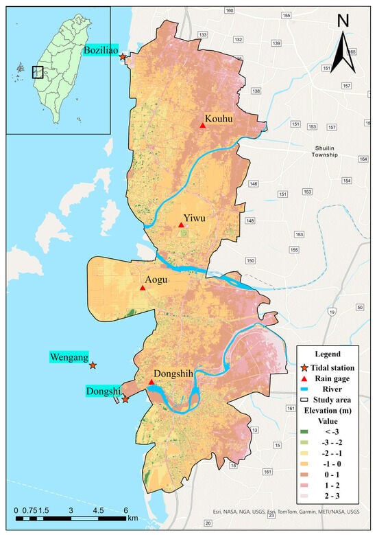
Figure 1.
Study area.
2.2. Data
Rainfall and tidal data from both the baseline and future periods, used as boundary conditions in the hydraulic model, were collected for flood simulations. For the baseline period, hourly rainfall data were retrieved from four automated meteorological stations (including the Kouhu, Yihu, Aogu, and Dongshi Stations), while the hourly tidal data were collected from three tidal stations (including the Boziliao, Wengang, and Dongshi Stations), as shown in Figure 1.
For future periods, gridded rainfall data were adopted from the Taiwan Climate Change Projection Information and Adaptation Knowledge Platform (TCCIP) [29]. These data are daily rainfall projections with a spatial resolution of 0.05° downscaled from the datasets released in the Intergovernmental Panel on Climate Change Sixth Assessment Report (IPCC AR6) [30] based on various General Circulation Models (GCMs) and Shared Socioeconomic Pathways (SSPs). This study adopted the SSP2-4.5 scenario, which represents a “middle-of-the-road” trajectory wherein greenhouse gas emissions are stabilized at moderate levels. Under this scenario, radiative forcing is projected to reach approximately 4.5 W/m2 by the end of the century (2100), leading to an estimated global mean temperature increase of about 2.7 °C relative to pre-industrial levels. Five GCMs (i.e., CanESM5, CMCC-CM2-SR5, MIROC6, MPI-ESM1-2-LR, and TaiESM1) were selected among the 29 GCMs included in AR6 based on their superior historical performance [31]. The daily rainfall projections from these models were subsequently disaggregated into hourly data to support future flood simulations. Considering the challenges and uncertainties in projecting future rainfall patterns under climate change, daily rainfall in this study was disaggregated into hourly data using a uniform distribution. For short-term analyses, this simplified method may introduce uncertainties in flood simulations due to the underestimation of peak rainfall intensities. However, for long-term trend analyses under climate change, the uncertainties associated with using uniform hourly rainfall patterns (internal variability) are considerably smaller than those arising from GCMs and emission scenarios [32]. Therefore, the use of a uniform disaggregation method may not introduce significant errors in this study.
For tidal data, the astronomical tidal hydrograph projected by the global tide model and the projected annual sea level rise values were combined to serve as the downstream boundary conditions for flood simulations. The astronomical tide projections were derived from the global tide model NAO99b, developed by the National Astronomical Observatory of Japan (NAO). This model integrates TOPEX/Poseidon satellite altimetry data [33] with a 2D hydrodynamic model [34] and data assimilation techniques to predict tidal characteristics for any given time and location. Sea level rise estimates were based on data from the IPCC AR6 and were obtained through the Sea Level Change Projection Tool offered by the National Aeronautics and Space Administration (NASA) [35]. This tool enables users to visualize projected sea level rise for any global region from 2020 to 2150 under various SSP scenarios. Table 1 shows the statistics of rainfall and tidal level used in this study.

Table 1.
Statistics of rainfall and tidal level.
3. Methodology
To analyze the interdecadal variations in compound flooding, a compound flood risk simulation framework was proposed using the consequence-based statistical method, as shown in Figure 2. In this framework, flood risk is defined as the probability of a flood hazard and is analyzed based on the exceedance probability of flood areas induced by the compound effects of rainfall and tide across historical and future periods following a three-step process. First, as indicated in green, land use data were processed for model construction, with different land use types represented by corresponding components in the SWMM. Rainfall and tidal data were collected and used as boundary conditions for flood simulations in both historical and future periods. Second, as indicated in yellow, the SWMM was applied to simulate the annual maximum flood areas (AMFA) for the baseline period (1995–2014) and four future periods, including the short-term (2021–2040), mid-term (2041–2060), medium–long-term (2061–2080), and long-term (2081–2100) periods, respectively. The flood area was defined as the area with water depths greater than 0.5 m, which corresponds to the threshold for eligibility for flood relief funds in Taiwan. Finally, as indicated in blue, the Mann-Kendall test, Theil-Sen estimator, and frequency analysis were conducted to evaluate the interdecadal variations in flood areas across the five periods.
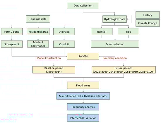
Figure 2.
Compound flood risk simulation framework.
3.1. Flood Risk Analysis
To assess flood risk, the values of AMFA should be determined and used for frequency analysis. In other words, candidate rainfall events likely to generate the largest flood area must be identified and used in flood simulations. To achieve this, the daily rainfall series were analyzed, and individual rainfall events were delineated by defining an event as starting when the daily rainfall exceeded 1 mm and ending when the daily rainfall fell below 1 mm on subsequent days. To select the most influential events, the three rainfall events with the highest daily rainfall in each year were selected and used as inputs for flood simulations, combined with the corresponding downstream tidal boundary conditions. Finally, the largest flood area generated in each year was extracted to determine the AMFA values, which were subsequently subjected to frequency analysis.
In this study, the frequency analysis was performed on the AMFA to examine variations in flood probability across different time periods and GCMs. Five probability density functions were compared to derive the cumulative distribution functions (CDFs) for flood areas, including the Normal, Log-Normal, Gamma, Gumbel, and Weibull distributions. The parameters of these distributions were estimated using the maximum likelihood estimation method, and the goodness-of-fit of the CDFs was evaluated using the Kolmogorov–Smirnov test [36].
3.2. SWMM Construction
The SWMM, developed by the U.S. Environmental Protection Agency (EPA), is used for simulating urban rainfall-runoff processes, infiltration, and drainage system hydraulics through the integration of hydrological and hydraulic models. In the hydrological model, the SCS Curve Number method and Manning’s equation are employed to calculate infiltration and runoff discharge, respectively. These values were assigned based on land use types, following the correspondence tables recommended in the SWMM User’s Manual [21], which have been well calibrated in previous studies. In the hydraulic model, the one-dimensional Saint-Venant equations are solved, and the runoff discharges are introduced to simulate unsteady flow conveyance across different elements. As a result, SWMM is suitable not only for short-term storm event simulations but also for long-term, multi-scenario, and multi-scale analyses. However, as a 1D model, SWMM requires specific component configurations tailored to different land uses to reasonably simulate the extent of 2D surface inundation. For this purpose, farms and ponds, residential areas, and drainage channels are represented as storage units, meshes of links and nodes, and conduits, respectively. These components are interconnected to simulate water exchanges among them, and corresponding flood areas are displayed when the water depth in a component exceeds the ground surface elevation. Details of the model setup are shown in Figure 3 and explained as follows:
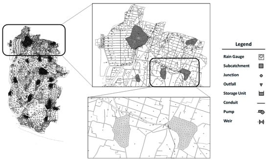
Figure 3.
Configuration of SWMM components in the study area.
- Farm and Pond: Farms and ponds are modeled as storage units interconnected by weirs to simulate flow exchange when water depths exceed the bund heights. A total of 1682 storage units and 3725 flow-exchange weirs were implemented for the farm and pond systems.
- Residential Area: To simulate surface flooding in detail, residential areas are discretized into small triangular mesh cells, each bounded by links and nodes. Rainfall-induced overland flow within each mesh cell drains to the associated node and is then conveyed through the connected links. A total of 8713 nodes and 12,360 links were implemented in the residential areas.
- Drainage Channel: Drainage channels are represented as conduits connected via junctions, which receive inflows from other components through weirs when water depths exceed embankment heights. A total of 1099 conduits, 1099 junctions, and 1233 flow-exchange weirs were established for the drainage network.
- Boundary Components: To simulate compound flooding induced by both rainfall and tides, rainfall-runoff hydrographs are assigned to each storage unit and node based on their corresponding subcatchment, while tidal levels are imposed at 12 outlet nodes located at the ends of rivers and drainage conduits.
3.3. Validation Indicators
To evaluate the accuracy of the simulation results, three indicators are employed for validation as follows: Overall Correct Rate (OCR), Hit Rate (HTR), and False Alarm Rate (FAR) [37,38].
where h represents the flooded area that is correctly predicted; m represents the flooded area that is not predicted; f represents the unflooded area that is falsely predicted as flooded; and c represents the area that is not flooded in both prediction and observation. All three indicators range between 0 and 1. The model demonstrates higher accuracy when the OCR and HTR approach 1 and the FAR approaches 0.
3.4. Mann-Kendall Test
The Mann-Kendall (MK) test [39] is a non-parametric method used to assess trends in time series data. Unlike linear regression, the MK test does not require the residuals to follow a normal distribution, making it suitable for datasets with small sample sizes and extreme values. As a result, it is widely applied in the analysis of long-term trends in meteorological, hydrological, and environmental data. The MK test estimates the trend of a time series using the following equation:
where and are the data values at times and , respectively; is the sample size; and is the number of positive differences minus the number of negative differences. The significance of can be determined by calculating the value of as follows:
where m is the number of groups with equal values in the sample, and is the number of repeated values in group . When the value of exceeds 0, an increasing trend is indicated, and vice versa. When and , the trend is considered significant and highly significant under the significance levels of and , respectively.
3.5. Theil–Sen Estimator
The Theil–Sen (TS) Estimator [40] calculates the slopes in a time series between all possible pairs of data values and estimates the median slope β using Equation (6). This method avoids the influence of extreme values in slope calculation and enhances the stability of the results.
where and are the data values at times and , respectively, and where is the Teil-Sen slope. If , an increasing trend is indicated, and vice versa.
4. Results
4.1. Validation
Figure 4 presents the simulated flood areas for Rainstorm 0612, with the validation indicators summarized in Table 2. The simulated flood areas were compared with the observed flood areas collected by local disaster prevention personnel through post-event field surveys. The average values of OCR, HTR, and FAR are 0.79, 0.81, and 0.18, respectively. These results indicate that approximately 80% of the actual flooded areas were correctly predicted by the model, while 18% of the unflooded areas were falsely identified as flooded. This inaccuracy may be attributed to the use of a 1D model in areas with complex 2D terrain features, which cannot be adequately represented by a 1D approach. However, the low FAR demonstrates that the high HTR value was not achieved through excessive overestimation but rather through a generally accurate delineation of flooded and unflooded areas. Overall, the model exhibits good consistency between simulation and observation for historical events and can be considered a reliable tool for future simulations under climate change scenarios.
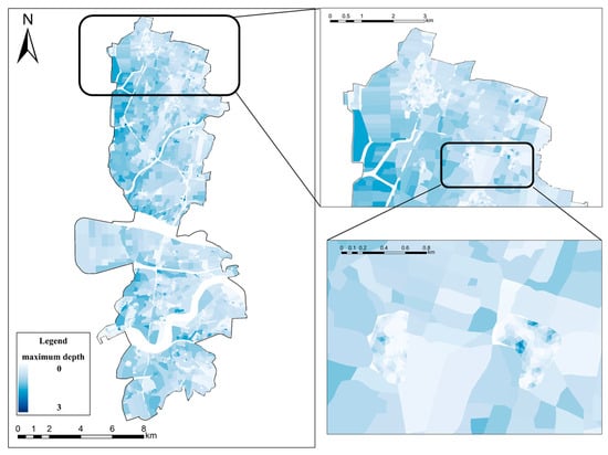
Figure 4.
Simulated flood areas for Rainstorm 0612.
Table 2.
Validation results for historical events.
4.2. Flood Area Trends
To examine future trends in flood areas, the AMFA values for each GCM were simulated using SWMM and are presented in Figure 5. In the figure, the average AMFA across all GCMs (dashed line) fluctuates but generally increases from 25 km2 in 2020 to 40 km2 in 2100. The shaded blue area represents the range of AMFA values, highlighting significant discrepancies among the GCM predictions. Figure 6 compares the average AMFA between the baseline and future periods under different GCMs. In the short-term and mid-term periods, CanESM5 predicts the lowest average AMFA, which is slightly below the baseline value of 29.15 km2. However, this trend reverses in the medium–long-term and long-term periods, during which CanESM5 shows a rapid increase in AMFA and surpasses the baseline. For some GCMs such as MPI-ESM1-2-LR and TaiESM1, the average AMFA remains consistently high across all future periods, suggesting that the impacts of climate change emerge early. Although discrepancies among GCMs are more pronounced in the short term, they converge in the long term, with an average increase of approximately 27.8% in AMFA by the end of the 21st century.
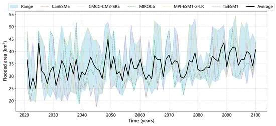
Figure 5.
Projected annual maximum flood areas under different GCMs.
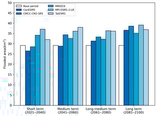
Figure 6.
Average annual maximum flood areas for the baseline and future periods under different GCMs.
Using the MK test and TS estimator, the trends of AMFA for different GCMs across future periods were quantified and are presented in Table 3. In the short-term and mid-term periods, the AMFA trends vary considerably among GCMs. For CanESM5 and TaiESM1, the MK test indicates a decreasing trend in the short term followed by an increasing trend in the mid-term period, whereas the opposite pattern is observed for MIROC6 and MPI-ESM1-2-LR. Despite these discrepancies, all GCMs project an increasing trend in AMFA during the medium–long-term and long-term periods. In particular, CMCC-CM2-SR5 exhibits a consistent upward trend across all future periods. Considering the entire projection horizon (2021–2100), all GCMs show an overall increase in AMFA, with especially notable increases in CanESM5 and CMCC-CM2-SR5. For these two models, the MK test results are highly significant, indicating an annual increase in flood area of approximately 0.162 km2. These findings suggest that, under the combined effects of increased rainfall and sea level rise, compound flooding is expected to intensify and expand over time, even though short-term fluctuations may occur.
Table 3.
Trends in the annual maximum flood area for different GCMs in the future.
4.3. Flood Risk Trends
For the future periods, the best-fit CDFs of flood areas derived from different GCMs are presented in Figure 7. The results show that the CDFs exhibit the greatest divergence in the short-term period (2021–2040) and gradually converge over time by shifting to the right, as seen in the long-term period (2081–2100). This rightward shift indicates a rising trend in flood risk under future climate scenarios. Overall, MPI-ESM1-2-LR projects the highest flood risk, with the largest flood areas corresponding to the same cumulative probability levels. In contrast, CanESM5 yields the lowest flood risk, particularly during the short-, mid-, and medium–long-term periods. Table 4 summarizes the variations in flood area return periods (FARPs) across the baseline and future periods. During the baseline period, the flood areas associated with return periods of 2, 5, 10, 20, 50, 100, and 200 years are 28.3, 32.1, 34.6, 37.0, 40.1, 42.4, and 44.7 km2, respectively. When applying these same flood area thresholds to the future scenarios, the corresponding FARPs become shorter for all GCMs, except for a slight increase in the short-term period under CanESM5. This general reduction in FARPs implies that flood events of a given magnitude are expected to occur more frequently, indicating a substantial increase in future flood risk. Moreover, the reduction in FARPs is more pronounced at higher return periods. Compared to the baseline, the FARPs for a 200-year flood area decreased by 187.9, 194.7, 179.1, 195.6, and 193.2 years in the long-term period for CanESM5, CMCC-CM2-SR5, MIROC6, MPI-ESM1-2-LR, and TaiESM1, respectively.
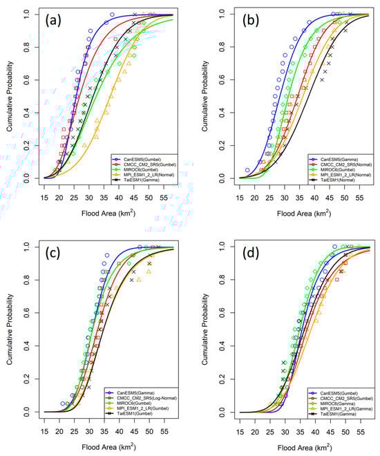
Figure 7.
Flood area CDFs for different GCMs in future periods: (a) 2021–2040, (b) 2041–2060, (c) 2061–2080, and (d) 2081–2100.
Table 4.
Variations in flood area return periods in the baseline and future periods.
5. Discussions
5.1. Novelty
- Event selection method: Instead of selecting events based on a fixed rainfall duration, this study selects events based on variable rainfall durations. This approach helps prevent the underestimation of annual flood magnitudes.
- Enhanced simulation efficiency: By representing 2D hydraulic structures as 1D components in SWMM, surface runoff can be simulated with reasonable accuracy while maintaining computational efficiency. Compared to just a few minutes for the 1D model, the computation time required by 2D models can significantly increase by a hundred times. If a 2D model is applied to simulate a 20-year period over the entire study area under five GCMs, it would require several months of computation, making it impractical. Therefore, the application of a 1D model is essential for long-term and large-scale simulations in future research.
- Risk assessment methodology: The occurrence probability of compound flooding is directly estimated using the return periods of flood areas, offering a more intuitive and practical alternative to traditional methods that rely on the joint probabilities of marginal flood-driving factors.
5.2. Limitations
- Expansion of GCM scenarios: This study employs five GCMs to estimate future com-pound flood risks. The results reveal substantial variability among GCMs in the short- to medium-term, although their long-term projections tend to converge. Differences among various GCMs in simulating circulation patterns and intensities lead to discrepancies in their predictions of the onset, break, and revival phases of the East Asian summer monsoon, which in turn results in substantial variations in rainfall forecasts over Taiwan [31]. Incorporating a broader range of GCMs would help better capture this uncertainty.
- Storm surge modeling: In this study, tidal boundary conditions were determined by the combination of astronomical tides and sea-level rise projections without including the typhoon-induced water level setup, which may underestimate the contribution of tidal surge to flooding. Future research could incorporate ocean model simulations that more accurately represent the influence of nearshore storm surges.
6. Conclusions
In this study, an innovative framework was developed that integrates SWMM with a consequence-based statistical method, allowing for the analysis of interdecadal variations in compound flood risk driven by both rainfall and tidal interactions under climate change. All GCMs indicated a rising probability of flood occurrence by the end of the century; however, trends varied across models during the short- and mid-term periods. The framework was demonstrated to be scalable and adaptable, offering a cost-effective approach for compound flood risk assessment that can be applied to other geographic regions with diverse hydrometeorological conditions. Based on the increasing trends identified by the model, adaptive strategies and mitigation measures are essential to address the growing impacts of compound flood risk under a changing climate.
Author Contributions
Conceptualization, J.-H.J.; methodology, J.-H.J. and Y.-M.W.; formal analysis, Y.-M.W.; writing—original draft: Y.-M.W. and T.-E.L.; writing—review and editing: J.-H.J., T.-H.C. and C.-H.H.; visualization, T.-E.L.; supervision, J.-H.J. All authors have read and agreed to the published version of the manuscript.
Funding
This research was funded by the National Science and Technology Council, Taiwan, grant No. NSTC 113-2625-M-006-021.
Data Availability Statement
The data that support the findings of this study are available upon reasonable request.
Conflicts of Interest
The authors declare no conflicts of interest.
References
- Jackson, L.P.; Grinsted, A.; Jevrejeva, S. 21st Century Sea-Level Rise in Line with the Paris Accord. Earth’s Future 2018, 6, 213–229. [Google Scholar] [CrossRef]
- Kulp, S.A.; Strauss, B.H. New elevation data triple estimates of global vulnerability to sea-level rise and coastal flooding. Nat. Commun. 2019, 10, 4844. [Google Scholar] [CrossRef] [PubMed]
- Boumis, G.; Moftakhari, H.R.; Moradkhani, H. Coevolution of Extreme Sea Levels and Sea-Level Rise Under Global Warming. Earth’s Future 2023, 11, e2023EF003649. [Google Scholar] [CrossRef]
- Rizzo, A.; Mattei, G.; Dumon Steenssens, L.; Anzidei, M.; Aucelli, P.P.C.; Alberti, T.; Antonioli, F.; Bezzi, A.; Bonaldo, D.; Fontolan, G.; et al. Methodological advances in sea level rise vulnerability assessment: Implications for sustainable coastal management in a climate change scenario. Ocean. Coast. Manag. 2025, 268, 107751. [Google Scholar] [CrossRef]
- Prein, A.F.; Rasmussen, R.M.; Ikeda, K.; Liu, C.; Clark, M.P.; Holland, G.J. The future intensification of hourly precipitation extremes. Nat. Clim. Change 2017, 7, 48–52. [Google Scholar] [CrossRef]
- Li, C.; Zwiers, F.; Zhang, X.; Chen, G.; Lu, J.; Li, G.; Norris, J.; Tan, Y.; Sun, Y.; Liu, M. Larger Increases in More Extreme Local Precipitation Events as Climate Warms. Geophys. Res. Lett. 2019, 46, 6885–6891. [Google Scholar] [CrossRef]
- Wahl, T.; Jain, S.; Bender, J.; Meyers, S.D.; Luther, M.E. Increasing risk of compound flooding from storm surge and rainfall for major US cities. Nat. Clim. Change 2015, 5, 1093–1097. [Google Scholar] [CrossRef]
- Valle-Levinson, A.; Olabarrieta, M.; Heilman, L. Compound flooding in Houston-Galveston Bay during Hurricane Harvey. Sci. Total Environ. 2020, 747, 141272. [Google Scholar] [CrossRef]
- Zscheischler, J.; Westra, S.; van den Hurk, B.J.J.M.; Seneviratne, S.I.; Ward, P.J.; Pitman, A.; AghaKouchak, A.; Bresch, D.N.; Leonard, M.; Wahl, T.; et al. Future climate risk from compound events. Nat. Clim. Change 2018, 8, 469–477. [Google Scholar] [CrossRef]
- Shen, Y.; Morsy, M.M.; Huxley, C.; Tahvildari, N.; Goodall, J.L. Flood risk assessment and increased resilience for coastal urban watersheds under the combined impact of storm tide and heavy rainfall. J. Hydrol. 2019, 579, 124159. [Google Scholar] [CrossRef]
- Hsiao, S.-C.; Chiang, W.-S.; Jang, J.-H.; Wu, H.-L.; Lu, W.-S.; Chen, W.-B.; Wu, Y.-T. Flood risk influenced by the compound effect of storm surge and rainfall under climate change for low-lying coastal areas. Sci. Total Environ. 2021, 764, 144439. [Google Scholar] [CrossRef] [PubMed]
- Bevacqua, E.; Maraun, D.; Vousdoukas, M.I.; Voukouvalas, E.; Vrac, M.; Mentaschi, L.; Widmann, M. Higher probability of compound flooding from precipitation and storm surge in Europe under anthropogenic climate change. Sci. Adv. 2019, 5, eaaw5531. [Google Scholar] [CrossRef] [PubMed]
- Xu, H.; Tian, Z.; Sun, L.; Ye, Q.; Ragno, E.; Bricker, J.; Mao, G.; Tan, J.; Wang, J.; Ke, Q.; et al. Compound flood impact of water level and rainfall during tropical cyclone periods in a coastal city: The case of Shanghai. Nat. Hazards Earth Syst. Sci. 2022, 22, 2347–2358. [Google Scholar] [CrossRef]
- Xu, K.; Zhuang, Y.; Bin, L.; Wang, C.; Tian, F. Impact assessment of climate change on compound flooding in a coastal city. J. Hydrol. 2023, 617, 129166. [Google Scholar] [CrossRef]
- Lian, J.; Xu, H.; Xu, K.; Ma, C. Optimal management of the flooding risk caused by the joint occurrence of extreme rainfall and high tide level in a coastal city. Nat. Hazards 2017, 89, 183–200. [Google Scholar] [CrossRef]
- Jang, J.-H.; Chang, T.-H. Flood risk estimation under the compound influence of rainfall and tide. J. Hydrol. 2022, 606, 127446. [Google Scholar] [CrossRef]
- Kumbier, K.; Carvalho, R.C.; Vafeidis, A.T.; Woodroffe, C.D. Investigating compound flooding in an estuary using hydrodynamic modelling: A case study from the Shoalhaven River, Australia. Nat. Hazards Earth Syst. Sci. 2018, 18, 463–477. [Google Scholar] [CrossRef]
- Zellou, B.; Rahali, H. Assessment of the joint impact of extreme rainfall and storm surge on the risk of flooding in a coastal area. J. Hydrol. 2019, 569, 647–665. [Google Scholar] [CrossRef]
- Saharia, A.M.; Zhu, Z.; Atkinson, J.F. Compound flooding from lake seiche and river flow in a freshwater coastal river. J. Hydrol. 2021, 603, 126969. [Google Scholar] [CrossRef]
- Yuan, J.; Zheng, F.; Duan, H.-F.; Deng, Z.; Kapelan, Z.; Savic, D.; Shao, T.; Huang, W.-M.; Zhao, T.; Chen, X. Numerical modelling and quantification of coastal urban compound flooding. J. Hydrol. 2024, 630, 130716. [Google Scholar] [CrossRef]
- Rossman, L.A. Storm Water Management Model User’s Manual Version 5.1—Manual; U.S. EPA Office of Research and Development: Washington, DC, USA, 2015. [Google Scholar]
- Han, H.; Kim, D.; Kim, H.S. Inundation Analysis of Coastal Urban Area under Climate Change Scenarios. Water 2022, 14, 1159. [Google Scholar] [CrossRef]
- Bibi, T.S.; Kara, K.G.; Bedada, H.J.; Bededa, R.D. Application of PCSWMM for assessing the impacts of urbanization and climate changes on the efficiency of stormwater drainage systems in managing urban flooding in Robe town, Ethiopia. J. Hydrol. Reg. Stud. 2023, 45, 101291. [Google Scholar] [CrossRef]
- Shi, S.; Yang, B.; Jiang, W. Numerical simulations of compound flooding caused by storm surge and heavy rain with the presence of urban drainage system, coastal dam and tide gates: A case study of Xiangshan, China. Coast. Eng. 2022, 172, 104064. [Google Scholar] [CrossRef]
- Ai, P.; Yuan, D.; Xiong, C. Copula-Based Joint Probability Analysis of Compound Floods from Rainstorm and Typhoon Surge: A Case Study of Jiangsu Coastal Areas, China. Sustainability 2018, 10, 2232. [Google Scholar] [CrossRef]
- Xu, H.; Xu, K.; Lian, J.; Ma, C. Compound effects of rainfall and storm tides on coastal flooding risk. Stoch. Environ. Res. Risk Assess. 2019, 33, 1249–1261. [Google Scholar] [CrossRef]
- Jane, R.; Cadavid, L.; Obeysekera, J.; Wahl, T. Multivariate statistical modelling of the drivers of compound flood events in south Florida. Nat. Hazards Earth Syst. Sci. 2020, 20, 2681–2699. [Google Scholar] [CrossRef]
- Lu, W.; Tang, L.; Yang, D.; Wu, H.; Liu, Z. Compounding Effects of Fluvial Flooding and Storm Tides on Coastal Flooding Risk in the Coastal-Estuarine Region of Southeastern China. Atmosphere 2022, 13, 238. [Google Scholar] [CrossRef]
- Taiwan Climate Change Projection Information and Adaptation Knowledge Platform. Available online: https://tccip.ncdr.nat.gov.tw/index_eng.aspx (accessed on 12 May 2025).
- Masson-Delmotte, V. Climate Change 2021: The Physical Science Basis: Working Group I Contribution to the Sixth Assessment Report of the Intergovernmental Panel on Climate Change, 1st ed.; Intergovernmental Panel on Climate Change. Working Group I, issuing body; Cambridge University Press: Cambridge, UK, 2023. [Google Scholar]
- Tung, Y.S.; Wang, S.Y.S.; Chu, J.L.; Wu, C.H.; Chen, Y.M.; Cheng, C.T.; Lin, L.Y. Projected increase of the East Asian summer monsoon (Meiyu) in Taiwan by climate models with variable performance. Meteorol. Appl. 2020, 27, e1886. [Google Scholar] [CrossRef]
- Hawkins, E.; Sutton, R. The potential to narrow uncertainty in projections of regional precipitation change. Clim. Dyn. 2011, 37, 407–418. [Google Scholar] [CrossRef]
- Morimoto, A.; Yanagi, T.; Kaneko, A. Tidal correction of altimetric data in the Japan Sea. J. Oceanogr. 2000, 56, 31–41. [Google Scholar] [CrossRef]
- Schwiderski, E.W. On charting global ocean tides. Rev. Geophys. (1985) 1980, 18, 243–268. [Google Scholar] [CrossRef]
- IPCC AR6 Sea Level Projection Tool. Available online: https://sealevel.nasa.gov/ipcc-ar6-sea-level-projection-tool (accessed on 12 May 2025).
- Chakravarti, I.M.; Laha, R.G.; Roy, J. Handbook of Methods of Applied Statistics: Techniques of Computation, Descriptive Methods, and Statistical Inference; Wiley: Hoboken, NJ, USA, 1967. [Google Scholar]
- Jang, J.H.; Chang, T.H.; Chen, W.B. Effect of inlet modelling on surface drainage in coupled urban flood simulation. J. Hydrol. 2018, 562, 168–180. [Google Scholar] [CrossRef]
- Jang, J.H.; Hsieh, C.T.; Chang, T.H. The importance of gully flow modelling to urban flood simulation. Urban Water J. 2019, 16, 377–388. [Google Scholar] [CrossRef]
- Marsick, A.; André, H.; Khelf, I.; Leclère, Q.; Antoni, J. Benefits of Mann–Kendall trend analysis for vibration-based condition monitoring. Mech. Syst. Signal Process. 2024, 216, 111486. [Google Scholar] [CrossRef]
- Bal, A. Improving the robustness of the theil-sen estimator using a simple heuristic-based modification. Symmetry 2024, 16, 698. [Google Scholar] [CrossRef]
Disclaimer/Publisher’s Note: The statements, opinions and data contained in all publications are solely those of the individual author(s) and contributor(s) and not of MDPI and/or the editor(s). MDPI and/or the editor(s) disclaim responsibility for any injury to people or property resulting from any ideas, methods, instructions or products referred to in the content. |
© 2025 by the authors. Licensee MDPI, Basel, Switzerland. This article is an open access article distributed under the terms and conditions of the Creative Commons Attribution (CC BY) license (https://creativecommons.org/licenses/by/4.0/).