


Regional Analysis of the Dependence of Peak-Flow Quantiles on Climate with Application to Adjustment to Climate Trends


Abstract
1. Introduction
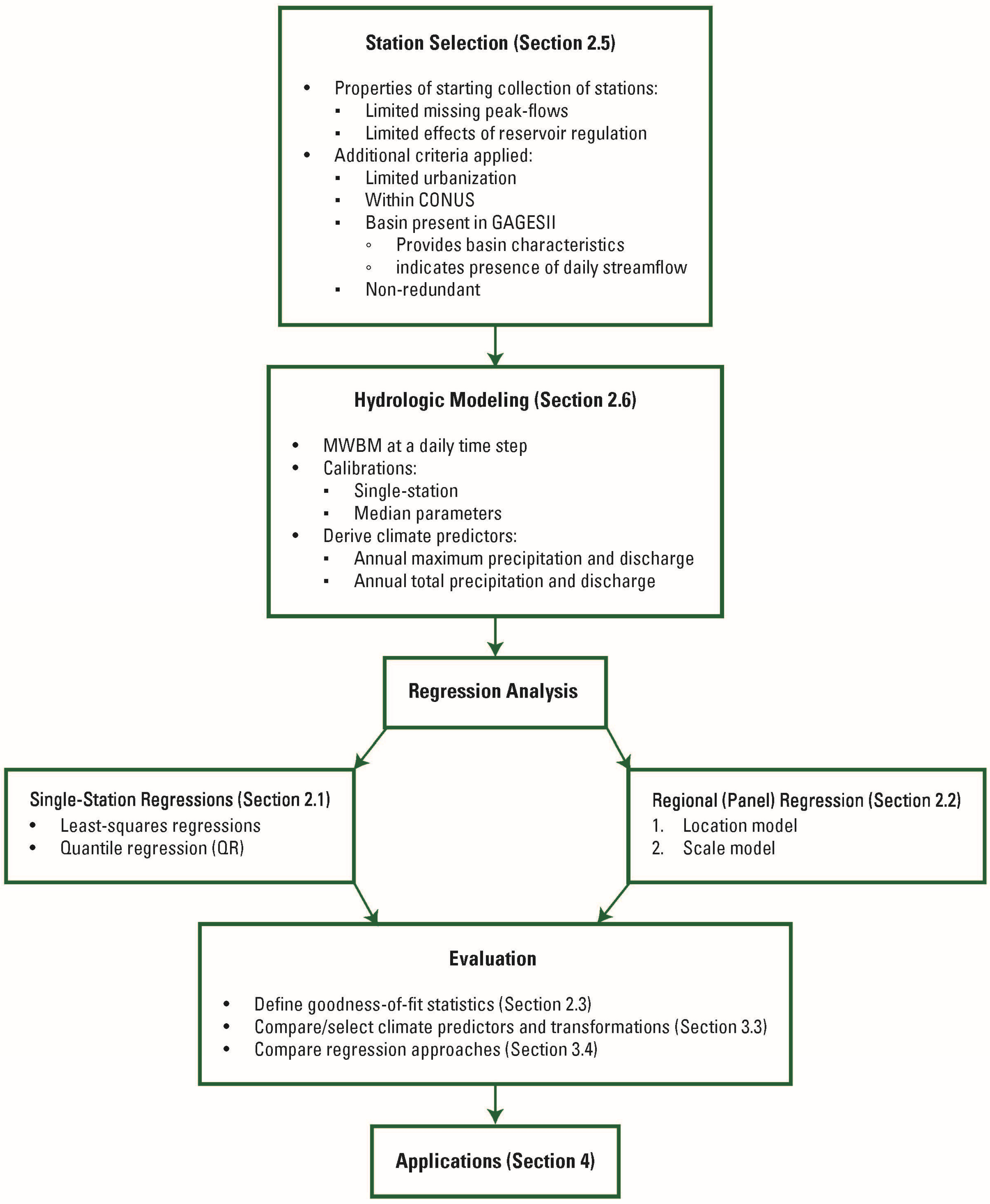
2. Materials and Methods
2.1. Single-Station Regression
2.2. Panel–Quantile Regression
- Compute the estimate of the location model coefficient by regressing the time-demeaned observations , where is the number of observations at the ith basin, on the time-demeaned explanatory (climate) variables, by least squares. Time-demeaning eliminates the location effects and the differences in means between the demeaned variables, so the regression only considers the variations “within” the data associated with each individual (i.e., station) i as they vary through time to compute .
- Compute the estimates of the location effects as , and define the residuals , which estimate , according to Equation (9).
- 3.
- Compute the estimate of the scale model coefficient by regressing the time-demeaned absolute residuals on the time-demeaned explanatory variables by least squares.
- 4.
- Compute the estimates of the scale effects as .
2.3. Goodness-of-Fit Statistics
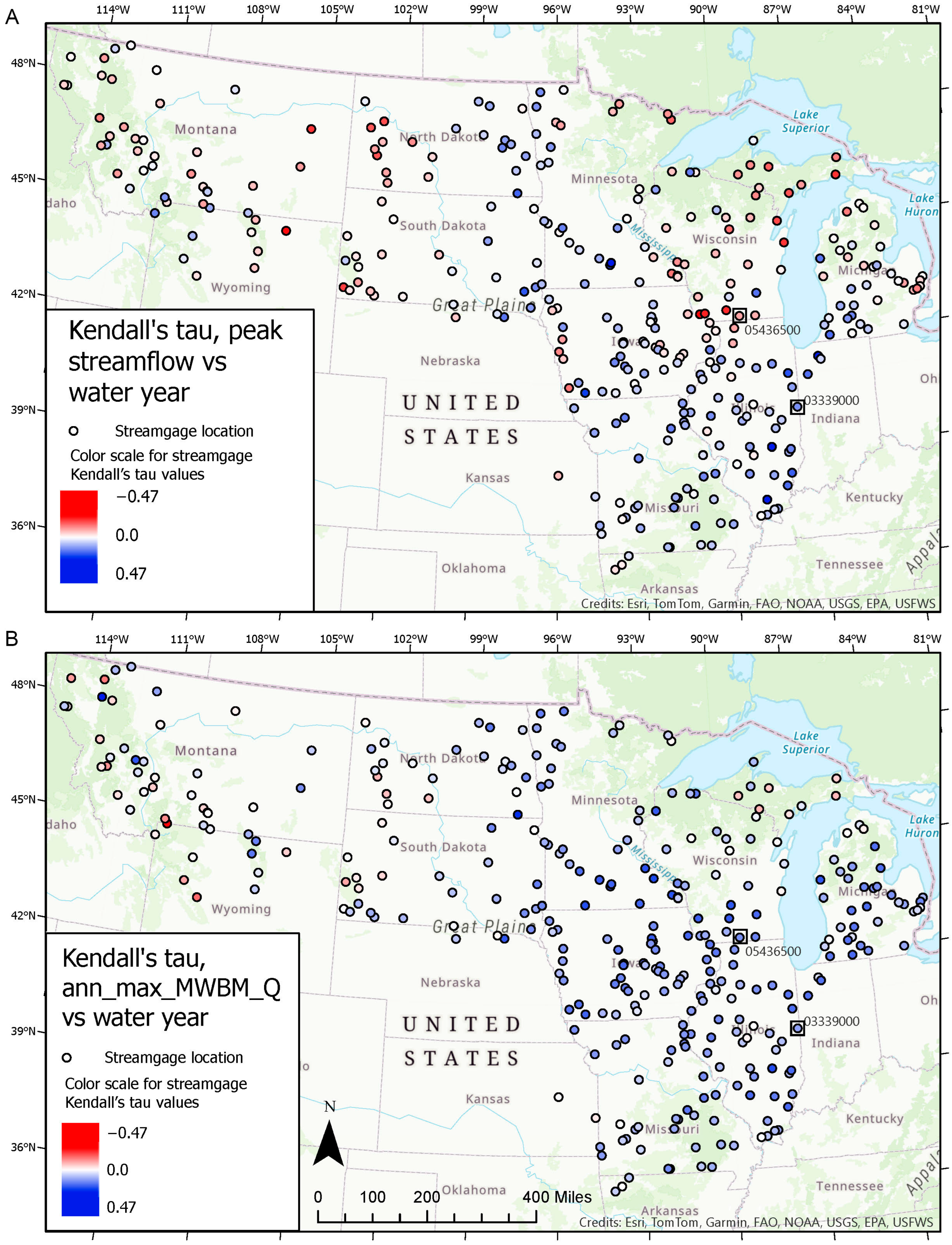
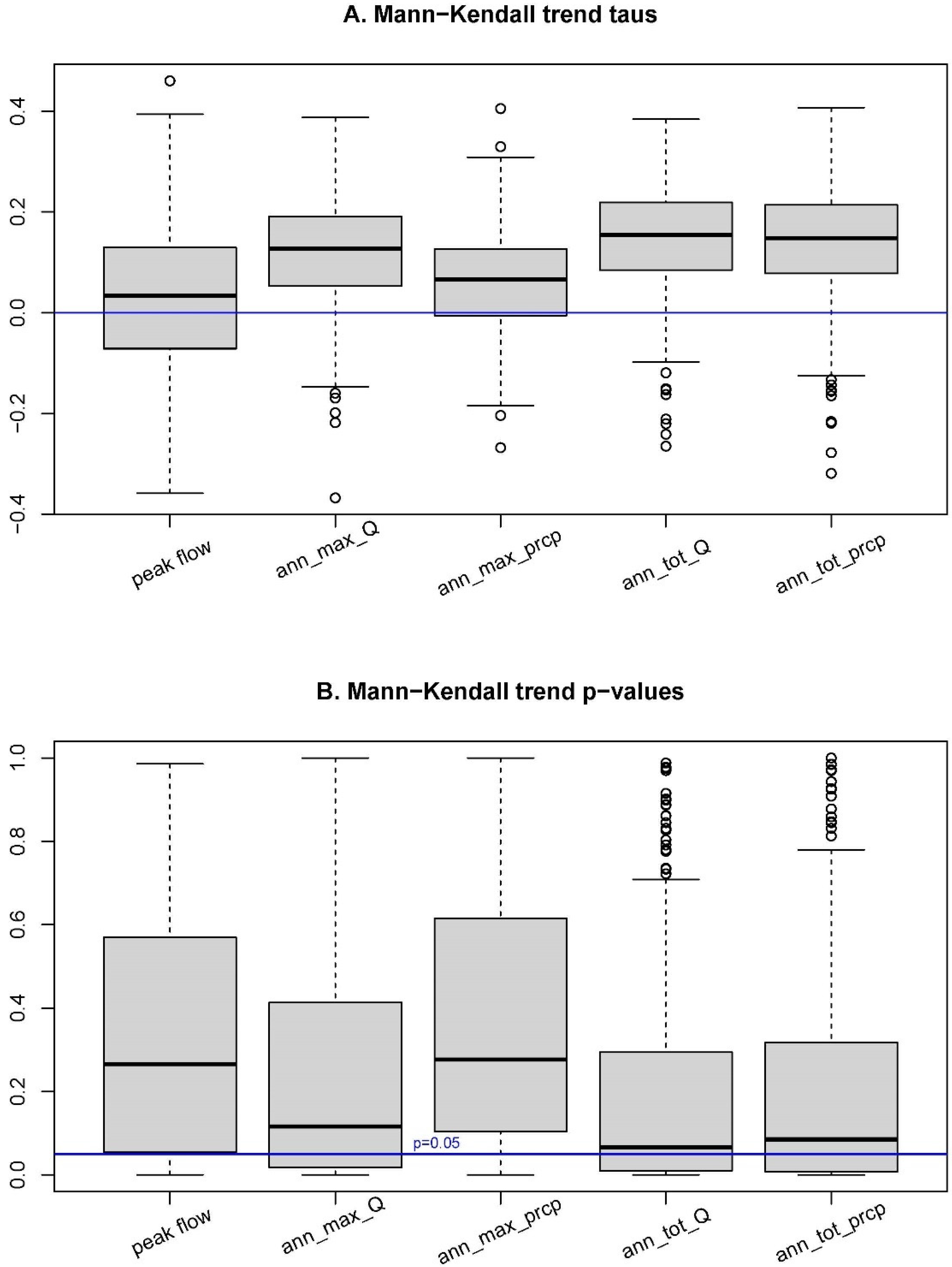
2.4. Computation of Temporal Trends
2.5. Station Selection and Peak-Flow Data
2.6. Computation of the Climate Predictors
3. Results
3.1. Temporal Trends
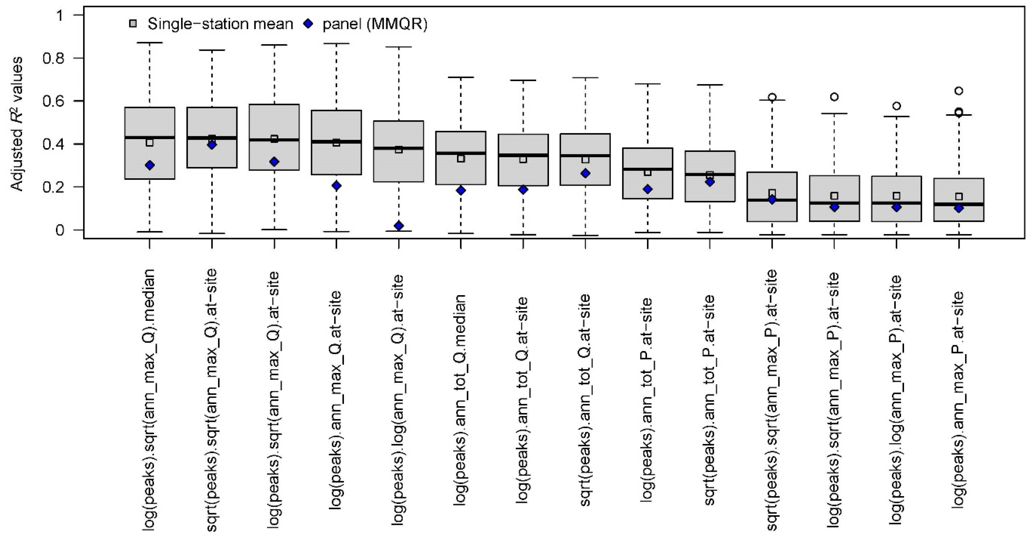
3.2. Goodness of Fit and the Selection of Climate Predictors and Regression Transformations
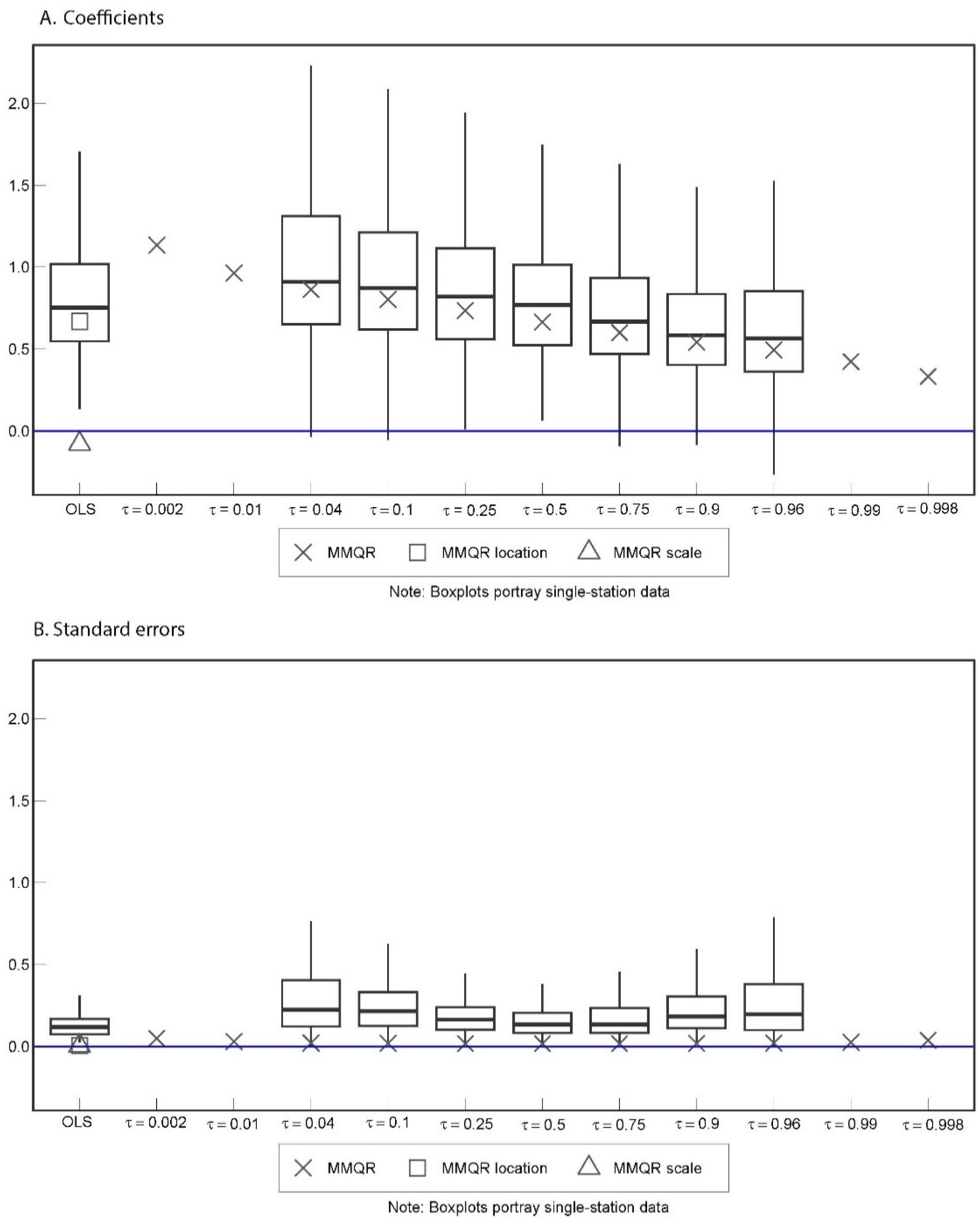
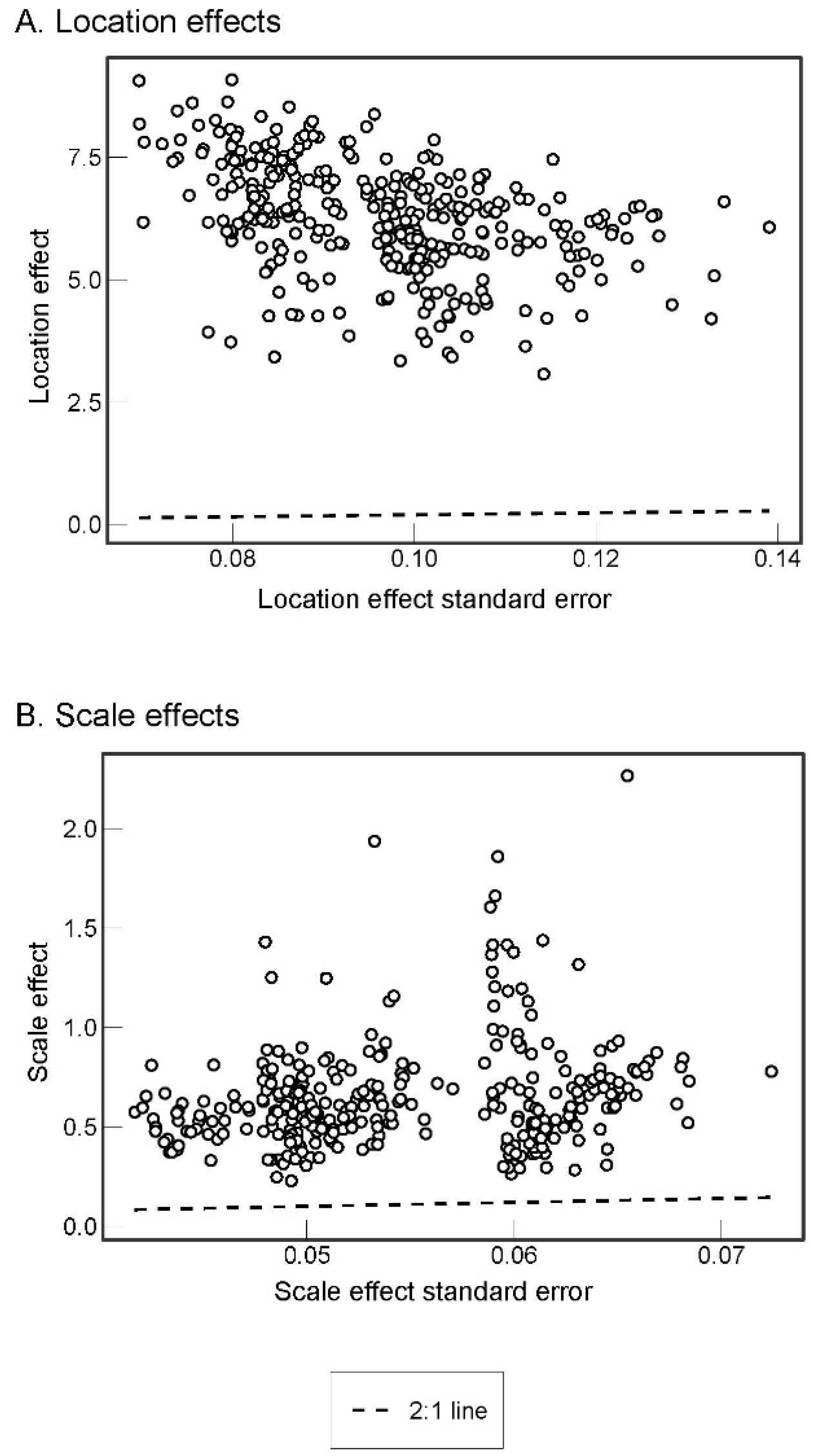
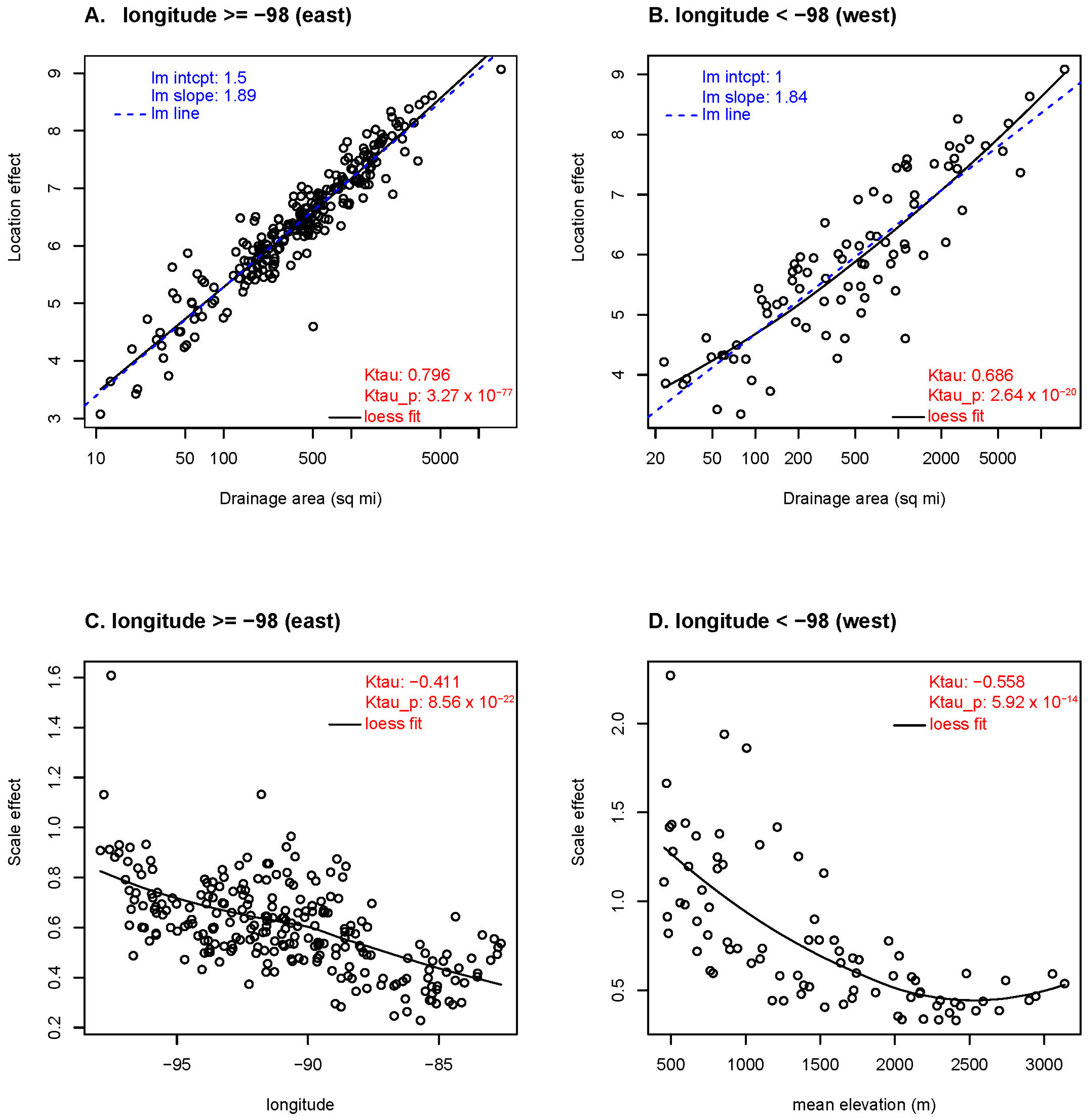
3.3. Regression Coefficients and Fixed Effects
3.4. Goodness of Fit and Comparison of Modeling Approaches
3.5. Results Summary
4. Applications
4.1. General Considerations
4.2. Estimation via Adjustment
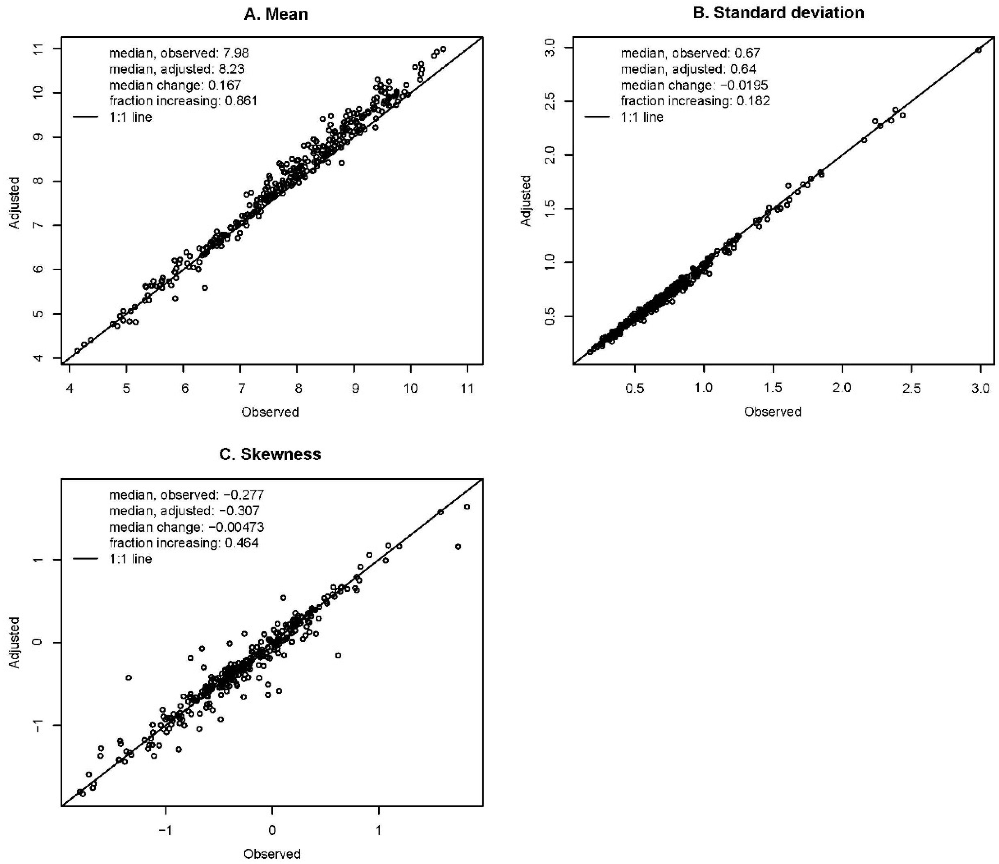
4.2.1. Method and Study-Wide Results
- Because the climate coefficients depend on , the next step is to estimate the value associated with each observed peak. This was achieved by interpolating among the conditional quantiles (Equation (5) for the single-station regressions and Equation (10) for the MMQR model); this interpolation was performed linearly in the space of log-transformed peaks versus the unit Gaussian quantile function with as the argument (equivalent to a set of straight-line segments on lognormal probability paper).
- Given the estimated value for each peak, estimate the coefficient value by interpolation among the fitted quantile coefficients and their values, which are given by (Equations (5) and (7)) for the single-station regressions and for the MMQR model (Equation (11)). This interpolation was performed linearly. Both interpolations are limited by the range of values, which are from to for the MMQR regressions, which is sufficient for all but the most extreme peaks, and from to for the single-station regressions. When the estimated value was beyond the most extreme value for which a coefficient estimate was available, the value at the nearest extreme was used.
- Given the coefficient value , the adjusted peak was computed as:where is the log of the observed peak-flow value for year t and station i, is adjusted to climate conditions during year T, is the estimated regression coefficient for the ith station for year t at the estimated non-exceedance probability value , is the smoothed climate for year t at station i, and is the smoothed climate value for year T at station i. For the applications considered here, the year to which the peaks were adjusted was taken as 2018, the end of the study period, so .
4.2.2. Example Basin: Vermilion River near Danville, Illinois
4.2.3. Example Basin: Sugar River near Brodhead, Wisconsin
5. Discussion and Conclusions
Supplementary Materials
Author Contributions
Funding
Data Availability Statement
Acknowledgments
Conflicts of Interest
Appendix A
References
- Hodgkins, G.A.; Dudley, R.W.; Archfield, S.A.; Renard, B. Effects of climate, regulation, and urbanization on historical flood trends in the United States. J. Hydrol. 2019, 573, 697–709. [Google Scholar] [CrossRef]
- Koutsoyiannis, D.; Montanari, A. Negligent killing of scientific concepts: The stationarity case. Hydrolog. Sci. J. 2015, 60, 1174–1183. [Google Scholar] [CrossRef]
- Milly, P.C.D.; Betancourt, J.; Falkenmark, M.; Hirsch, R.M.; Kundzewicz, Z.W.; Lettenmaier, D.P.; Stouffer, R.J. Stationarity is dead: Whither water management? Science 2008, 319, 573–574. [Google Scholar] [CrossRef] [PubMed]
- Milly, P.C.D.; Betancourt, J.; Falkenmark, M.; Hirsch, R.M.; Kundzewicz, Z.W.; Lettenmaier, D.P.; Stouffer, R.J.; Dettinger, M.D.; Krysanova, V. On critiques of “Stationarity is dead: Whither water management?”. Water Resour. Res. 2015, 51, 7785–7789. [Google Scholar] [CrossRef]
- Ryberg, K.R. (Ed.) Attribution of Monotonic Trends and Change Points in Peak Streamflow Across the Conterminous United States Using a Multiple Working Hypotheses Framework, 1941–2015 and 1966–2015; Professional Paper 1869; U.S. Geological Survey: Reston, VA, USA, 2022. [Google Scholar] [CrossRef]
- Salas, J.D.; Obeysekera, J.; Vogel, R.M. Techniques for assessing water infrastructure for nonstationary extreme events: A review. Hydrolog. Sci. J. 2018, 63, 325–352. [Google Scholar] [CrossRef]
- Salas, J.D.; Obeysekera, J. Revisiting the concepts of return period and risk for nonstationary hydrologic extreme events. J. Hydrol. Eng. 2014, 19, 554–568. [Google Scholar] [CrossRef]
- Serago, J.M.; Vogel, R.M. Parsimonious nonstationary flood frequency analysis. Adv. Water Resour. 2018, 112, 1–16. [Google Scholar] [CrossRef]
- Serinaldi, F.; Kilsby, C.G. Stationarity is undead—Uncertainty dominates the distribution of extremes. Adv. Water Resour. 2015, 77, 17–36. [Google Scholar] [CrossRef]
- Villarini, G.; Serinaldi, F.; Smith, J.A.; Krajewski, W.F. On the stationarity of annual flood peaks in the continental United States during the 20th century. Water Resour. Res. 2009, 45, W08417. [Google Scholar] [CrossRef]
- Villarini, G.; Taylor, S.; Wobus, C.; Vogel, R.; Hecht, J.; White, K.; Baker, B.; Gilroy, K.; Olsen, J.R.; Raff, D. Floods and Nonstationarity: A Review; Civil Works Technical Series 2018–01; U.S. Army Corps of Engineers: Washington, DC, USA, 2018; Available online: https://usace.contentdm.oclc.org/digital/collection/p266001coll1/id/6036/ (accessed on 21 March 2019).
- Vogel, R.M.; Yaindl, C.; Walter, M. Nonstationarity—Flood magnification and recurrence reduction factors in the United States. J. Am. Water Resour. Assoc. 2011, 47, 464–474. [Google Scholar] [CrossRef]
- Archfield, S.A.; Hirsch, R.M.; Viglione, A.; Blöschl, G. Fragmented patterns of flood change across the United States. Geophys. Res. Lett. 2016, 43, 10232–10239. [Google Scholar] [CrossRef] [PubMed]
- Berghuijs, W.R.; Aalbers, E.E.; Larsen, J.R.; Trancoso, R.; Woods, R.A. Recent changes in extreme floods across multiple continents. Environ. Res. Lett. 2017, 12, 114035. [Google Scholar] [CrossRef]
- Hirsch, R.M.; Ryberg, K.R. Has the magnitude of floods across the USA changed with global CO2 levels? Hydrolog. Sci. J. 2012, 57, 1–9. [Google Scholar] [CrossRef]
- Hodgkins, G.A.; Whitfield, P.H.; Burn, D.H.; Hannaford, J.; Renard, B.; Stahl, K.; Fleig, A.K.; Madsen, H.; Mediero, L.; Korhonen, J.; et al. Climate-driven variability in the occurrence of major floods across North America and Europe. J. Hydrol. 2017, 552, 704–717. [Google Scholar] [CrossRef]
- Sharma, A.; Wasko, C.; Lettenmaier, D.P. If precipitation extremes are increasing, why aren’t floods? Water Resour. Res. 2018, 54, 8545–8551. [Google Scholar] [CrossRef]
- Koutsoyiannis, D. Hurst-Kolmogorov dynamics and uncertainty. J. Am. Water Resour. Assoc. 2011, 47, 481–495. [Google Scholar] [CrossRef]
- Lins, H.F.; Cohn, T.A. Stationarity—Wanted dead or alive? J. Am. Water Resour. Assoc. 2011, 47, 475–480. [Google Scholar] [CrossRef]
- Payton, E.A.; Pinson, A.O.; Asefa, T.; Condon, L.E.; Dupigny-Giroux, L.-A.L.; Harding, B.L.; Kiang, J.; Lee, D.H.; McAfee, S.A.; Pflug, J.M.; et al. Ch. 4. Water. In Fifth National Climate Assessment; Crimmins, A.R., Avery, C.W., Easterling, D.R., Kunkel, K.E., Stewart, B.C., Maycock, T.K., Eds.; U.S. Global Change Research Program: Washington, DC, USA, 2023. [Google Scholar] [CrossRef]
- Blum, A.G.; Ferraro, P.J.; Archfield, S.A.; Ryberg, K.R. Causal effect of impervious cover on annual flood magnitude for the United States. Geophys. Res. Lett. 2020, 47, e2019GL086480. [Google Scholar] [CrossRef]
- Espey, W.H., Jr.; Winslow, D.E. Urban flood frequency characteristics. J. Hydr. Div.-ASCE 1974, 100, 279–293. [Google Scholar] [CrossRef]
- Hollis, G.E. The effect of urbanization on floods of different recurrence interval. Water Resour. Res. 1975, 11, 431–435. [Google Scholar] [CrossRef]
- Konrad, C.P. Effects of Urban Development on Floods; Fact Sheet 076–03; U.S. Geological Survey: Reston, VA, USA, 2003. Available online: https://pubs.usgs.gov/fs/fs07603/ (accessed on 7 May 2009).
- Over, T.M.; Saito, R.J.; Soong, D.T. Adjusting Annual Maximum Peak Discharges at Selected Stations in Northeastern Illinois for Changes in Land-Use Conditions; Scientific Investigations Report 2016–5049; U.S. Geological Survey: Reston, VA, USA, 2016. [Google Scholar] [CrossRef]
- Over, T.M.; Saito, R.J.; Veilleux, A.G.; O’Shea, P.S.; Sharpe, J.B.; Soong, D.T.; Ishii, A.L. Estimation of Peak Discharge Quantiles for Selected Annual Exceedance Probabilities in Northeastern Illinois; Scientific Investigations Report 2016–5050; U.S. Geological Survey: Reston, VA, USA, 2021. [Google Scholar] [CrossRef]
- Over, T.; Marti, M.; Ortiz, J.; Podzorski, H. The joint effect of changes in urbanization and climate on trends in floods: A comparison of panel and single-station quantile regression approaches. J. Hydrol. 2025, 648, 132281. [Google Scholar] [CrossRef]
- Sauer, V.B.; Thomas, W.O., Jr.; Stricker, V.A.; Wilson, K.V. Flood Characteristics of Urban Watersheds in the United States; Water-Supply Paper 2207; U.S. Geological Survey: Reston, VA, USA, 1983. [Google Scholar] [CrossRef]
- Yang, W.; Yang, H.; Yang, D.; Hou, A. Causal effects of dams and land cover changes on flood changes in mainland China. Hydrol. Earth Syst. Sci. 2021, 25, 2705–2720. [Google Scholar] [CrossRef]
- Wasko, C.; Westra, S.; Nathan, R.; Orr, H.G.; Villarini, G.; Villalobos Herrera, R.; Fowler, H.J. Incorporating climate change in flood estimation guidance. Philos. Trans. R. Soc. A 2021, 379, 20190548. [Google Scholar] [CrossRef] [PubMed]
- England, J.F., Jr.; Cohn, T.A.; Faber, B.A.; Stedinger, J.R.; Thomas, W.O., Jr.; Veilleux, A.G.; Kiang, J.E.; Mason, R.R., Jr. Guidelines for Determining Flood Flow Frequency—Bulletin 17C (Ver. 1.1, May 2019); Techniques and Methods 4-B5; U.S. Geological Survey: Reston, VA, USA, 2019. [Google Scholar] [CrossRef]
- François, B.; Schlef, K.E.; Wi, S.; Brown, C.M. Design considerations for riverine floods in a changing climate—A review. J. Hydrol. 2019, 574, 557–573. [Google Scholar] [CrossRef]
- Kilgore, R.; Thomas, W.O., Jr.; Douglass, S.; Webb, B.; Hayhoe, K.; Stoner, A.; Jacobs, J.M.; Thompson, D.; Hermann, G.; Douglas, E.; et al. Applying Climate Change Information to Hydrologic and Coastal Design of Transportation Infrastructure [Design Practices Guide]; National Cooperative Highway Research Program, Transportation Research Board: Washington, DC, USA, 2019; p. 145. Available online: https://apps.trb.org/cmsfeed/trbnetprojectdisplay.asp?projectid=4046 (accessed on 28 November 2023).
- Kilgore, R.; Thomas, W.O., Jr.; Douglass, S.; Webb, B.; Hayhoe, K.; Stoner, A.; Jacobs, J.; Thompson, D.B.; Hermann, G.R.; Douglas, E.; et al. Applying Climate Change Information to Hydrologic and Coastal Design of Transportation Infrastructure [Final Report]; National Cooperative Highway Research Program, Transportation Research Board: Washington, DC, USA, 2019; p. 201. Available online: https://apps.trb.org/cmsfeed/trbnetprojectdisplay.asp?projectid=4046 (accessed on 28 November 2023).
- Madsen, H.; Lawrence, D.; Lang, M.; Martinkova, M.; Kjeldsen, T.R. Review of trend analysis and climate change projections of extreme precipitation and floods in Europe. J. Hydrol. 2014, 519 Pt D, 3634–3650. [Google Scholar] [CrossRef]
- Schlef, K.E.; François, B.; Brown, C. Comparing flood projection approaches across hydro-climatologically diverse United States river basins. Water Resour. Res. 2021, 57, e2019WR025861. [Google Scholar] [CrossRef]
- Slater, L.J.; Anderson, B.; Buechel, M.; Dadson, S.; Han, S.; Harrigan, S.; Kelder, T.; Kowal, K.; Lees, T.; Matthews, T.; et al. Nonstationary weather and water extremes: A review of methods for their detection, attribution, and management. Hydrol. Earth Syst. Sci. 2021, 25, 3897–3935. [Google Scholar] [CrossRef]
- Schlef, K.E.; François, B.; Robertson, A.W.; Brown, C. A general methodology for climate-informed approaches to long-term flood projection—Illustrated with the Ohio River Basin. Water Resour. Res. 2018, 54, 9321–9341. [Google Scholar] [CrossRef]
- Glas, R.; Hecht, J.; Simonson, A.; Gazoorian, C.; Schubert, C. Adjusting design floods for urbanization across groundwater-dominated watersheds of Long Island, NY. J. Hydrol. 2023, 618, 129194. [Google Scholar] [CrossRef]
- Hecht, J.S.; Barth, N.A.; Ryberg, K.R.; Gregory, A.E. Simulation experiments comparing nonstationary design-flood adjustments based on observed annual peak flows in the conterminous United States. J. Hydrol. X 2022, 17, 100115. [Google Scholar] [CrossRef]
- Hecht, J.S.; Vogel, R.M. Updating urban design floods for changes in central tendency and variability using regression. Adv. Water Resour. 2020, 136, 103484. [Google Scholar] [CrossRef]
- Luke, A.; Vrugt, J.A.; AghaKouchak, A.; Matthew, R.; Sanders, B.F. Predicting nonstationary flood frequencies: Evidence supports an updated stationarity thesis in the United States. Water Resour. Res. 2017, 53, 5469–5494. [Google Scholar] [CrossRef]
- Benson, M. Factors Influencing the Occurrence of Floods in a Humid Region of Diverse Terrain; Water Supply Paper 1580-B; U.S. Geological Survey: Washington, DC, USA, 1963. [Google Scholar] [CrossRef]
- Dalrymple, T. Flood-Frequency Analyses, Manual of Hydrology: Part 3; Water Supply Paper 1543-A; U.S. Geological Survey: Washington, DC, USA, 1960. [Google Scholar] [CrossRef]
- Stedinger, J.R.; Vogel, R.M.; Foufoula-Georgiou, E. Frequency analysis of extreme events. In Handbook of Hydrology; Maidment, D.R., Ed.; McGraw-Hill: New York, NY, USA, 1993; pp. 18.1–18.66. ISBN 0070397325. [Google Scholar]
- Eng, K.; Chen, Y.-Y.; Kiang, J.E. User’s Guide to the Weighted-Multiple-Linear Regression Program (WREG Version 1.0); Techniques and Methods 4-A8; U.S. Geological Survey: Reston, VA, USA, 2009. [Google Scholar] [CrossRef]
- Farmer, W.H.; Kiang, J.E.; Feaster, T.D.; Eng, K. Regionalization of Surface-Water Statistics Using Multiple Linear Regression (Ver. 1.1, February 2021); Techniques and Methods, 4-A12; U.S. Geological Survey: Reston, VA, USA, 2021. [Google Scholar] [CrossRef]
- Singh, R.; Wagener, T.; van Werkhoven, K.; Mann, M.E.; Crane, R. A trading-space-for-time approach to probabilistic continuous streamflow predictions in a changing climate—Accounting for changing watershed behavior. Hydrol. Earth Syst. Sci. 2011, 15, 3591–3603. [Google Scholar] [CrossRef]
- Singh, R.; van Werkhoven, K.; Wagener, T. Hydrological impacts of climate change in gauged and ungauged watersheds of the Olifants basin: A trading-space-for-time approach. Hydrolog. Sci. J. 2014, 59, 29–55. [Google Scholar] [CrossRef]
- Berghuijs, W.R.; Woods, R.A. Correspondence: Space-time asymmetry undermines water yield assessment. Nat. Commun. 2016, 7, 11603. [Google Scholar] [CrossRef] [PubMed]
- Perdigão, R.A.P.; Blöschl, G. Spatiotemporal flood sensitivity to annual precipitation: Evidence for landscape-climate coevolution. Water Resour. Res. 2014, 50, 5492–5509. [Google Scholar] [CrossRef]
- Wooldridge, J.M. Introductory Econometrics: A Modern Approach, 5th ed.; South-Western, Cengage Learning: Mason, OH, USA, 2013; p. 881. ISBN 1111531048. [Google Scholar]
- Anderson, B.J.; Slater, L.J.; Dadson, S.J.; Blum, A.G.; Prosdocimi, I. Statistical attribution of the influence of urban and tree cover change on streamflow: A comparison of large sample statistical approaches. Water Resour. Res. 2022, 58, e2021WR030742. [Google Scholar] [CrossRef]
- Bassiouni, M.; Vogel, R.M.; Archfield, S.A. Panel regressions to estimate low-flow response to rainfall variability in ungaged basins. Water Resour. Res. 2016, 52, 9470–9494. [Google Scholar] [CrossRef]
- Ferreira, S.; Ghimire, R. Forest cover, socioeconomics, and reported flood frequency in developing countries. Water Resour. Res. 2012, 48, 2011WR011701. [Google Scholar] [CrossRef]
- Steinschneider, S.; Yang, Y.-C.E.; Brown, C. Panel regression techniques for identifying impacts of anthropogenic landscape change on hydrologic response. Water Resour. Res. 2013, 49, 7874–7886. [Google Scholar] [CrossRef]
- Greene, W.H. Econometric Analysis, 3rd ed.; Prentice-Hall: Upper Saddle River, NJ, USA, 1997; p. 1075. ISBN 0023466022. [Google Scholar]
- Koenker, R.; Bassett, G. Regression quantiles. Econometrica 1978, 46, 33–50. [Google Scholar] [CrossRef]
- Frumento, P.; Bottai, M. Parametric modeling of quantile regression coefficient functions. Biometrics 2016, 72, 74–84. [Google Scholar] [CrossRef]
- Ouali, D.; Chebana, F.; Ouarda, T.B.M.J. Quantile regression in regional frequency analysis: A better exploitation of the available information. J. Hydrometeorol. 2016, 17, 1869–1883. [Google Scholar] [CrossRef]
- Sankarasubramanian, A.; Lall, U. Flood quantiles in a changing climate: Seasonal forecasts and causal relation. Water Resour. Res. 2003, 39, 1134. [Google Scholar] [CrossRef]
- Konrad, C.; Restivo, D. Assessment and significance of the frequency domain for trends in annual peak streamflow. J. Flood Risk Manag. 2021, 14, e12761. [Google Scholar] [CrossRef]
- Nasri, B.; Bouezmarni, T.; St-Hilaire, A.; Ouarda, T.B.M.J. Non-stationary hydrologic frequency analysis using B-spline quantile regression. J. Hydrol. 2017, 554, 532–544. [Google Scholar] [CrossRef]
- Qu, C.; Li, J.; Yan, L.; Yan, P.; Cheng, F.; Lu, D. Non-stationary flood frequency analysis using cubic b-spline-based GAMLSS model. Water 2020, 12, 1867. [Google Scholar] [CrossRef]
- Ryberg, K.R. (Ed.) Peak Streamflow Trends and Their Relation to Changes in Climate in Illinois, Iowa, Michigan, Minnesota, Missouri, Montana, North Dakota, South Dakota, and Wisconsin; Scientific Investigations Report 2023–5064; U.S. Geological Survey: Reston, VA, USA, 2024. [Google Scholar] [CrossRef]
- Villarini, G.; Smith, J.A.; Baeck, M.L.; Vitolo, R.; Stephenson, D.B.; Krajewski, W.F. On the frequency of heavy rainfall for the Midwest of the United States. J. Hydrol. 2011, 400, 103–120. [Google Scholar] [CrossRef]
- Villarini, G.; Slater, L.J. Examination of changes in annual maximum gauge height in the continental United States using quantile regression. J. Hydrol. Eng. 2018, 23, 06017010. [Google Scholar] [CrossRef]
- Awasthi, C.; Archfield, S.A.; Reich, B.J.; Sankarasubramanian, A. Beyond simple trend tests: Detecting significant changes in design-flood quantiles. Geophys. Res. Lett. 2023, 50, e2023GL103438. [Google Scholar] [CrossRef]
- Koenker, R. Quantile regression for longitudinal data. J. Multivar. Anal. 2004, 91, 74–89. [Google Scholar] [CrossRef]
- Galvao, A.F.; Kato, K. Quantile regression methods for longitudinal data. In Handbook of Quantile Regression; Koenker, R., Chernozhukov, V., He, X., Peng, L., Eds.; CRC Press, Taylor and Francis Group: Boca Raton, FL, USA, 2017; pp. 363–380. ISBN 978-1498725286. [Google Scholar]
- Canay, I.A. A simple approach to quantile regression for panel data. Econom. J. 2011, 14, 368–386. [Google Scholar] [CrossRef]
- Machado, J.A.F.; Santos Silva, J.M.C. Quantiles via moments. J. Econom. 2019, 213, 145–173. [Google Scholar] [CrossRef]
- R Core Team. R: A Language and Environment for Statistical Computing (Version 4.3.1) [Computer Software]; R Foundation for Statistical Computing: Vienna, Austria, 2023; Available online: https://www.R-project.org (accessed on 28 November 2023).
- Koenker, R. quantreg: Quantile Regression [R]. 2023. Available online: https://CRAN.R-project.org/package=quantreg (accessed on 28 November 2023).
- Dhaene, G.; Jochmans, K. Split-panel jackknife estimation of fixed-effect models. Rev. Econ. Stud. 2015, 82, 991–1030. [Google Scholar] [CrossRef]
- Croissant, Y.; Millo, G. Panel data econometrics in R: The plm package. J. Stat. Softw. 2008, 27, 1–43. [Google Scholar] [CrossRef]
- Millo, G. Robust standard error estimators for panel models: A unifying approach. J. Stat. Softw. 2017, 82, 1–27. [Google Scholar] [CrossRef]
- Arellano, M. Computing robust standard errors for within-groups estimators. Oxf. Bull. Econ. Stat. 1987, 49, 431–434. [Google Scholar] [CrossRef]
- Marti, M.K.; Podzorski, H.L.; Over, T.M. Data for Regional Analysis of the Dependence of Peak-Flow Quantiles on Climate with Application to Adjustment to Climate Trends [Dataset]; U.S. Geological Survey: Reston, VA, USA, 2025. [Google Scholar] [CrossRef]
- Helsel, D.R.; Hirsch, R.M.; Ryberg, K.R.; Archfield, S.A.; Gilroy, E.J. Statistical Methods in Water Resources; Techniques and Methods 4-A3; U.S. Geological Survey: Reston, VA, USA, 2020. [Google Scholar] [CrossRef]
- He, X. Quantile curves without crossing. Am. Stat. 1997, 51, 186–192. [Google Scholar] [CrossRef]
- Zhao, Q. Restricted regression quantiles. J. Multivar. Anal. 2000, 72, 78–99. [Google Scholar] [CrossRef]
- Mann, H.B. Nonparametric tests against trend. Econometrica 1945, 13, 245–259. [Google Scholar] [CrossRef]
- Dakota Water Science Center. Flood-Frequency Analysis in the Midwest: Addressing Potential Nonstationary Annual Peak-Flow Records. U.S. Geological Survey. Available online: https://www.usgs.gov/centers/dakota-water/science/flood-frequency-analysis-midwest-addressing-potential-nonstationary (accessed on 21 June 2024).
- Ryberg, K.R.; Over, T.M.; Levin, S.B.; Heimann, D.C.; Barth, N.A.; Marti, M.K.; O’Shea, P.S.; Sanocki, C.A.; Williams-Sether, T.J.; Wavra, H.N.; et al. Introduction and methods of analysis for peak streamflow trends and their relation to changes in climate in Illinois, Iowa, Michigan, Minnesota, Missouri, Montana, North Dakota, South Dakota, and Wisconsin. In Ch. A of Peak Streamflow Trends and Their Relation to Changes in Climate in Illinois, Iowa, Michigan, Minnesota, Missouri, Montana, North Dakota, South Dakota, and Wisconsin; Scientific Investigations Report 2023–5064; Ryberg, K.R., Ed.; U.S. Geological Survey: Reston, VA, USA, 2024. [Google Scholar] [CrossRef]
- Ryberg, K.R.; Williams-Sether, T. Peak streamflow trends in North Dakota and their relation to changes in climate, water years 1921–2020. In Ch. H of Peak Streamflow Trends and Their Relation to Changes in Climate in Illinois, Iowa, Michigan, Minnesota, Missouri, Montana, North Dakota, South Dakota, and Wisconsin; Scientific Investigations Report 2023–5064; Ryberg, K.R., Ed.; U.S. Geological Survey: Reston, VA, USA, 2025. [Google Scholar] [CrossRef]
- Marti, M.K.; Ryberg, K.R. Method for Identification of Reservoir Regulation Within U.S. Geological Survey Streamgage Basins in the Central United States Using a Decadal Dam Impact Metric; Open-File Report 2023–1034; U.S. Geological Survey: Reston, VA, USA, 2023. [Google Scholar] [CrossRef]
- Dewitz, J. National Land Cover Database (NLCD) 2019 Products (Ver. 2.0, June 2021) [Dataset]; U.S. Geological Survey data release; U.S. Geological Survey: Reston, VA, USA, 2021. [Google Scholar] [CrossRef]
- Wickham, J.; Stehman, S.V.; Sorenson, D.G.; Gass, L.; Dewitz, J.A. Thematic accuracy assessment of the NLCD 2019 land cover for the conterminous United States. GISci. Remote Sens. 2023, 60, 2181143. [Google Scholar] [CrossRef] [PubMed]
- Falcone, J. GAGES-II: Geospatial Attributes of Gages for Evaluating Streamflow [Dataset]; U.S. Geological Survey: Reston, VA, USA, 2011. [Google Scholar] [CrossRef]
- Veilleux, A.G. Bayesian GLS Regression for Regionalization of Hydrologic Statistics, Floods, and Bulletin 17 Skew. Master’s Thesis, Cornell University, Ithaca, NY, USA, 2009. Available online: https://ecommons.cornell.edu/bitstream/handle/1813/13819/Veilleux,%20Andrea.pdf?sequence=1 (accessed on 19 February 2015).
- Marti, M.K.; Wavra, H.N.; Over, T.M.; Ryberg, K.R.; Podzorski, H.L.; Chen, Y.R. Peak Streamflow Data, Climate Data, and Results from Investigating Hydroclimatic Trends and Climate Change Effects on Peak Streamflow in the Central United States, 1920-2020 [Dataset]; U.S. Geological Survey: Reston, VA, USA, 2024. [Google Scholar] [CrossRef]
- Dahl, T.E. Status and Trends of Prairie Wetlands in the United States 1997 to 2009; U.S. Department of the Interior, Fish and Wildlife Service, Ecological Services: Washington, DC, USA, 2014; p. 67. Available online: https://www.fws.gov/sites/default/files/documents/Status-and-Trends-of-Prairie-Wetlands-in-the-United-States-1997-to-2009.pdf (accessed on 28 August 2024).
- Pierce, D.W.; Su, L.; Cayan, D.R.; Risser, M.D.; Livneh, B.; Lettenmaier, D.P. An extreme-preserving long-term gridded daily precipitation dataset for the conterminous United States. J. Hydrometeorol. 2021, 22, 1883–1895. [Google Scholar] [CrossRef]
- Livneh, B.; Rosenberg, E.A.; Lin, C.; Nijssen, B.; Mishra, V.; Andreadis, K.M.; Maurer, E.P.; Lettenmaier, D.P. A long-term hydrologically based dataset of land surface fluxes and states for the conterminous United States: Update and extensions. J. Clim. 2013, 26, 9384–9392. [Google Scholar] [CrossRef]
- McCabe, G.J.; Markstrom, S.L. A Monthly Water-Balance Model Driven by a Graphical User Interface; Open-File Report 2007–1088; U.S. Geological Survey: Reston, VA, USA, 2007. Available online: https://pubs.usgs.gov/of/2007/1088/pdf/of07-1088_508.pdf (accessed on 14 December 2007).
- McCabe, G.J.; Wolock, D.M. Independent effects of temperature and precipitation on modeled runoff in the conterminous United States. Water Resour. Res. 2011, 47, W11522. [Google Scholar] [CrossRef]
- U.S. Geological Survey. USGS Water Data for the Nation—U.S. Geological Survey National Water Information System Database [National Water Information System—Web Interface]; U.S. Geological Survey: Reston, VA, USA, 2024. [CrossRef]
- Zambrano-Bigiarini, M.; Rojas, R. hydroPSO: Particle Swarm Optimisation, with Focus on Environmental Models (Version R Package Version 0.5-1) [Computer Software]. 2020. Available online: https://github.com/hzambran/hydroPSO (accessed on 23 January 2025).
- Gupta, H.V.; Kling, H.; Yilmaz, K.K.; Martinez, G.F. Decomposition of the mean squared error and NSE performance criteria: Implications for improving hydrological modelling. J. Hydrol. 2009, 377, 80–91. [Google Scholar] [CrossRef]
- Kling, H.; Fuchs, M.; Paulin, M. Runoff conditions in the upper Danube basin under an ensemble of climate change scenarios. J. Hydrol. 2012, 424–425, 264–277. [Google Scholar] [CrossRef]
- Seager, R.; Lis, N.; Feldman, J.; Ting, M.; Williams, A.P.; Nakamura, J.; Liu, H.; Henderson, N. Whither the 100th Meridian? The once and future physical and human geography of America’s arid–humid divide. Part I: The story so far. Earth Interact. 2018, 22, 1–22. [Google Scholar] [CrossRef]
- Seager, R.; Feldman, J.; Lis, N.; Ting, M.; Williams, A.P.; Nakamura, J.; Liu, H.; Henderson, N. Whither the 100th Meridian? The once and future physical and human geography of America’s arid–humid divide. Part II: The meridian moves east. Earth Interact. 2018, 22, 1–24. [Google Scholar] [CrossRef]
- Cleveland, W.S.; Grosse, E.; Shyu, W.M. Local regression models. In Statistical Models in S; Chambers, J.M., Hastie, T.J., Eds.; Chapman and Hall/CRC Press: New York, NY, USA, 1992; pp. 309–376. ISBN 0534167640. [Google Scholar]
- Gebert, W.A.; Garn, H.S.; Rose, W.J. Changes in Streamflow Characteristics in Wisconsin as Related to Precipitation and Land Use; Scientific Investigations Report 2015–5140; U.S. Geological Survey: Reston, VA, USA, 2016. [Google Scholar] [CrossRef]
- Gebert, W.A.; Krug, W.R. Streamflow trends in Wisconsin’s Driftless Area. J. Am. Water Resour. Assoc. 1996, 32, 733–744. [Google Scholar] [CrossRef]
- Juckem, P.F.; Hunt, R.J.; Anderson, M.P.; Robertson, D.M. Effects of climate and land management change on streamflow in the driftless area of Wisconsin. J. Hydrol. 2008, 355, 123–130. [Google Scholar] [CrossRef]
- Park, D.; Markus, M. Analysis of a changing hydrologic flood regime using the Variable Infiltration Capacity model. J. Hydrol. 2014, 515, 267–280. [Google Scholar] [CrossRef]
- Potter, K.W. Hydrological impacts of changing land management practices in a moderate-sized agricultural catchment. Water Resour. Res. 1991, 27, 845–855. [Google Scholar] [CrossRef]
- Levin, S.B. Peak streamflow trends in Wisconsin and their relation to changes in climate, water years 1921–2020, U.S. Geological Survey. In Ch. J of Peak Streamflow Trends and Their Relation to Changes in Climate in Illinois, Iowa, Michigan, Minnesota, Missouri, Montana, North Dakota, South Dakota, and Wisconsin; Scientific Investigations Report 2023–5064; Ryberg, K.R., Ed.; U.S. Geological Survey: Reston, VA, USA, 2024. [Google Scholar] [CrossRef]


| Quantile | Years of Record | Drainage Area (sq. km.) | Mean Annual Precipitation (MAP) (mm) | Aridity = PET/MAP | Mean Elevation (m) |
|---|---|---|---|---|---|
| 0% (min.) | 38 | 28.0 | 317 | 0.249 | 145 |
| 5% | 45 | 107 | 419 | 0.559 | 197 |
| 10% | 47 | 163 | 496 | 0.657 | 217 |
| 25% | 48 | 485 | 649 | 0.727 | 274 |
| 50% | 69 | 1116 | 824 | 0.791 | 349 |
| 75% | 73 | 2501 | 913 | 0.917 | 503 |
| 90% | 93.1 | 4688 | 1062 | 1.281 | 1661 |
| 95% | 97 | 6808 | 1123 | 1.497 | 2182 |
| 100% (max.) | 98 | 38,732 | 1755 | 1.964 | 3137 |
| Parameter Name | Definition | Range of Values Considered in This Study | Minimum Calibrated Value | Median Calibrated Value | Maximum Calibrated Value |
|---|---|---|---|---|---|
| Train | Temperature above which all precipitation is rain | 0 to 10 degC | 0 | 4.26 | 10 |
| Tsnow | Temperature below which all precipitation is snow | −10 to 0 degC | −10 | −1.60 | 0 |
| Melt factor | Upper bound of fraction of snow storage that can melt each day | 0.01 to 0.2 | 0.01 | 0.154 | 0.2 |
| STC | Soil water storage capacity | 20 to 500 mm | 20 | 329 | 500 |
| Drofrac | Fraction of rain that runs off directly, i.e., during the same day as it occurs. | 0 to 0.50 | 0 | 0.0132 | 0.282 |
| Rofrac | Fraction of excess soil moisture that runs off each day. | 0.01 to 0.3 | 0.01 | 0.0851 | 0.3 |
| Peak Flow vs. Water Year| trend ≤ 0 | Peak Flow vs. Water Year| trend > 0 | ann_max_Q vs. Water Year| trend ≤ 0 | ann_max_Q vs. Water Year| trend > 0 | ann_max_prcp vs. Water Year| trend ≤ 0 | ann_max_prcp vs. Water Year| trend > 0 | ann_tot_Q vs. Water Year| trend ≤ 0 | ann_tot_Q vs. Water Year| trend > 0 | ann_tot_prcp vs. Water Year| trend ≤ 0 | ann_tot_prcp vs. Water Year| trend > 0 | |
|---|---|---|---|---|---|---|---|---|---|---|
| p ≤ 0.05 | 0.079 | 0.161 | 0.012 | 0.348 | 0.009 | 0.139 | 0.012 | 0.412 | 0.012 | 0.418 |
| p > 0.05 | 0.352 | 0.409 | 0.133 | 0.506 | 0.267 | 0.585 | 0.109 | 0.467 | 0.079 | 0.491 |
| Total | 0.430 | 0.570 | 0.145 | 0.855 | 0.276 | 0.724 | 0.121 | 0.879 | 0.091 | 0.909 |
| Peak Flow | ann_max_Q | ann_max_prcp | ann_tot_Q | ann_tot_prcp | |
|---|---|---|---|---|---|
| peak flow | 1 | 0.284 | 0.153 | 0.160 | 0.148 |
| ann_max_Q | 0.284 | 1 | 0.440 | 0.606 | 0.550 |
| ann_max_prcp | 0.153 | 0.440 | 1 | 0.331 | 0.337 |
| ann_tot_Q | 0.160 | 0.606 | 0.331 | 1 | 0.769 |
| ann_tot_prcp | 0.148 | 0.550 | 0.337 | 0.769 | 1 |
| tau (1) | Single-Station Mean | Single-Station Q1 | Single-Station Median | Single-Station Median SE | Single-Station Median t Statistic | Single-Station Q3 | Single-Station Coeff .v0_SE_ frac2 (2) | Single-Station Coeff. vMMQR_SE_ frac2 (3) | MMQR Coeff | MMQR Coeff Robust SE | MMQR Coeff t Statistic | q (tau) |
|---|---|---|---|---|---|---|---|---|---|---|---|---|
| lm/plm | 0.848 | 0.548 | 0.751 | 0.118 | 6.4 | 1.017 | 0.985 | 0.488 | 0.668 | 0.017 | 38.2 | NA |
| MMQR scale | NA | NA | NA | NA | NA | NA | NA | NA | −0.0782 | 0.0066 | NA | NA |
| 0.002 | NA | NA | NA | NA | NA | NA | NA | NA | 1.134 | 0.049 | 23.0 | −5.33 |
| 0.01 | NA | NA | NA | NA | NA | NA | NA | NA | 0.964 | 0.030 | 31.8 | −3.51 |
| 0.04 | 1.074 | 0.651 | 0.911 | 0.223 | 4.1 | 1.311 | 0.800 | 0.636 | 0.863 | 0.022 | 39.4 | −2.35 |
| 0.1 | 1.000 | 0.619 | 0.872 | 0.215 | 4.1 | 1.212 | 0.867 | 0.579 | 0.802 | 0.019 | 42.2 | −1.63 |
| 0.25 | 0.907 | 0.559 | 0.819 | 0.165 | 5.0 | 1.115 | 0.936 | 0.555 | 0.735 | 0.018 | 41.8 | −0.83 |
| 0.5 | 0.838 | 0.524 | 0.769 | 0.134 | 5.8 | 1.015 | 0.955 | 0.530 | 0.665 | 0.017 | 38.6 | 0.04 |
| 0.75 | 0.760 | 0.469 | 0.667 | 0.133 | 5.0 | 0.934 | 0.921 | 0.464 | 0.600 | 0.017 | 34.5 | 0.84 |
| 0.9 | 0.686 | 0.403 | 0.584 | 0.184 | 3.2 | 0.836 | 0.773 | 0.488 | 0.542 | 0.019 | 29.3 | 1.54 |
| 0.96 | 0.666 | 0.362 | 0.564 | 0.196 | 2.9 | 0.852 | 0.664 | 0.506 | 0.494 | 0.021 | 23.6 | 2.13 |
| 0.99 | NA | NA | NA | NA | NA | NA | NA | NA | 0.423 | 0.027 | 15.6 | 2.93 |
| 0.998 | NA | NA | NA | NA | NA | NA | NA | NA | 0.333 | 0.038 | 8.8 | 4.00 |
| Statistic | tau0.04 | tau0.1 | tau0.25 | tau0.5 | tau0.75 | tau0.9 | tau0.96 | |
|---|---|---|---|---|---|---|---|---|
| Single-station | Min. | 0 | 0 | 0 | 0 | 0 | 0 | 0 |
| MMQR | Min. | 6.89 × 10⁻⁷ | 2.18 × 10⁻⁶ | 4.46 × 10⁻⁶ | 1.93 × 10⁻⁵ | 5.73 × 10⁻⁶ | 7.70 × 10⁻⁸ | 2.18 × 10⁻⁶ |
| MMQR-LOOCV | Min. | 2.89 × 10⁻⁶ | 3.09 × 10⁻⁵ | 3.76 × 10⁻⁵ | 3.82 × 10⁻⁵ | 3.31 × 10⁻⁵ | 5.33 × 10⁻⁶ | 1.65 × 10⁻⁶ |
| Single-station | Q1 | 0.0178 | 0.0318 | 0.0504 | 0.0581 | 0.0473 | 0.0303 | 0.0166 |
| MMQR | Q1 | 0.0214 | 0.0373 | 0.0612 | 0.0695 | 0.0563 | 0.0346 | 0.0190 |
| MMQR-LOOCV | Q1 | 0.0360 | 0.0719 | 0.1327 | 0.1599 | 0.1130 | 0.0542 | 0.0241 |
| Single-station | Median | 0.0316 | 0.0616 | 0.1110 | 0.1388 | 0.1080 | 0.0596 | 0.0297 |
| MMQR | Median | 0.0358 | 0.0692 | 0.1243 | 0.1552 | 0.1177 | 0.0637 | 0.0318 |
| MMQR-LOOCV | Median | 0.0619 | 0.1312 | 0.2541 | 0.3295 | 0.2467 | 0.1181 | 0.0506 |
| Single-station | Mean | 0.0454 | 0.0943 | 0.1694 | 0.2073 | 0.1605 | 0.0861 | 0.0405 |
| MMQR | Mean | 0.0553 | 0.1065 | 0.1852 | 0.2238 | 0.1717 | 0.0939 | 0.0468 |
| MMQR-LOOCV | Mean | 0.0990 | 0.1812 | 0.3096 | 0.3931 | 0.3464 | 0.2355 | 0.1493 |
| Single-station | Q3 | 0.0517 | 0.1095 | 0.2108 | 0.2704 | 0.2055 | 0.1047 | 0.0491 |
| MMQR | Q3 | 0.0583 | 0.1208 | 0.2308 | 0.2930 | 0.2210 | 0.1113 | 0.0521 |
| MMQR-LOOCV | Q3 | 0.0908 | 0.1994 | 0.4030 | 0.5450 | 0.4742 | 0.2661 | 0.1093 |
| Single-station | Max. | 2.62 | 3.49 | 4.97 | 4.28 | 2.49 | 2.16 | 1.40 |
| MMQR | Max. | 4.05 | 4.72 | 4.86 | 4.21 | 2.65 | 2.92 | 2.88 |
| MMQR-LOOCV | Max. | 7.47 | 7.75 | 7.14 | 5.26 | 2.86 | 2.99 | 2.93 |
| By Quantile (tau) | By Observation | ||||||||||||
|---|---|---|---|---|---|---|---|---|---|---|---|---|---|
| 0.002 | 0.01 | 0.04 | 0.1 | 0.25 | 0.5 | 0.75 | 0.9 | 0.96 | 0.99 | 0.998 | Minimum | Mean | |
| Single-station | NA | NA | 1 | 0.979 | 0.993 | 0.996 | 0.996 | 0.991 | 0.980 | NA | NA | 0.286 | 0.9907 |
| MMQR | 1 | 0.9985 | 0.9989 | 0.9990 | 0.9992 | 0.9993 | 0.9993 | 0.9993 | 0.9993 | 0.9992 | 0.9993 | 0.0909 | 0.9992 |
| MMQR-LOOCV | 1 | 0.9982 | 0.9988 | 0.9989 | 0.9992 | 0.9992 | 0.9993 | 0.9993 | 0.9993 | 0.9992 | 0.9993 | 0.0909 | 0.9991 |
Disclaimer/Publisher’s Note: The statements, opinions and data contained in all publications are solely those of the individual author(s) and contributor(s) and not of MDPI and/or the editor(s). MDPI and/or the editor(s) disclaim responsibility for any injury to people or property resulting from any ideas, methods, instructions or products referred to in the content. |
© 2025 by the authors. Licensee MDPI, Basel, Switzerland. This article is an open access article distributed under the terms and conditions of the Creative Commons Attribution (CC BY) license (https://creativecommons.org/licenses/by/4.0/).
Share and Cite
Over, T.; Marti, M.; Podzorski, H. Regional Analysis of the Dependence of Peak-Flow Quantiles on Climate with Application to Adjustment to Climate Trends. Hydrology 2025, 12, 119. https://doi.org/10.3390/hydrology12050119
Over T, Marti M, Podzorski H. Regional Analysis of the Dependence of Peak-Flow Quantiles on Climate with Application to Adjustment to Climate Trends. Hydrology. 2025; 12(5):119. https://doi.org/10.3390/hydrology12050119
Chicago/Turabian StyleOver, Thomas, Mackenzie Marti, and Hannah Podzorski. 2025. "Regional Analysis of the Dependence of Peak-Flow Quantiles on Climate with Application to Adjustment to Climate Trends" Hydrology 12, no. 5: 119. https://doi.org/10.3390/hydrology12050119
APA StyleOver, T., Marti, M., & Podzorski, H. (2025). Regional Analysis of the Dependence of Peak-Flow Quantiles on Climate with Application to Adjustment to Climate Trends. Hydrology, 12(5), 119. https://doi.org/10.3390/hydrology12050119