Abstract
Accurate measurement and understanding of the spatiotemporal distribution of soil water content (SWC) are crucial in various environmental and agricultural sectors. The present study implements a novel precision agriculture (PA) approach under sugarbeet field conditions of two moisture-irrigation treatments with two subfactors, clay loam (CL) and clay (C) soils, for geostatistics modeling (seven models’ evaluation) of time domain reflectometry (TDR) multisensor network measurements. Two different sensor calibration methods (M1 and M2) were trialed, as well as the results of laboratory soil analysis for geospatial two-dimensional (2D) imaging for accurate GIS maps of root zone moisture profiles, granular, and hydraulic profiles in multiple soil layers (0–75 cm depth). Modeling results revealed that the best-fitted semi-variogram models for the granular attributes were circular, exponential, pentaspherical, and spherical, while for hydraulic attributes were found to be exponential, circular, and spherical models. The results showed that kriging modeling, spatial and temporal imaging for accurate profile SWC (m3·m−3) maps, the exponential model was identified as the most appropriate with TDR sensors using calibration M1, and the exponential and spherical models were the most appropriate when using calibration M2. The resulting PA profile maps depict spatiotemporal soil water variability with very high resolutions at the centimeter scale. The best validation measures of PA profile SWC maps obtained were Nash-Sutcliffe model efficiency NSE = 0.6657, MPE = 0.00013, RMSE = 0.0385, MSPE = −0.0022, RMSSE = 1.6907, ASE = 0.0418, and MSDR = 0.9695. The sensor results using calibration M2 were found to be more valuable in environmental irrigation decision-making for a more accurate and timely decision on actual crop irrigation, with the lowest statistical and geostatistical errors. The best validation measures for accurate profile SWC (m3·m−3) maps obtained for clay loam over clay soils. Visualizing the SWC results and their temporal changes via root zone profile geostatistical maps assists farmers and scientists in making informed and timely environmental irrigation decisions, optimizing energy, saving water, increasing water-use efficiency and crop production, reducing costs, and managing water–soil resources sustainably.
1. Introduction
In the soil-water-plant-atmosphere environment (SWPAE), SWC is one of the essential factors that is the fundamental nexus of the hydrological cycle in terrestrial ecosystems, affecting soil evaporation, land surface water runoff, infiltration, and energy balance on the land top layer [1,2,3,4,5]. In addition, SWC, or soil moisture (SM), is one of the principal water sources for plant development and defines plant functionality, morphology, and productivity [2,5,6,7,8]. Over the last thirty-five years, there has been a growing trend in studies addressing the interactions between SM, climate, plants, and landscapes [2,6,8,9,10,11,12,13,14,15,16], but in situ datasets linking physiographical and vegetal traits to longitudinal and time-series patterns of soil moisture are scarce. Furthermore, understanding the dynamics of SM in diverse ecosystems is crucial, as the water quantity inside the soil governs multiple ecosystem services and functions, like water runoff, soil fertility, microbial degradation, and overall net production [3,4]. In dryland ecosystems, most precipitation events are quite small, usually <5 mm [17]; and because of the often-small volume of precipitation, only a few centimeters of the topsoil are moist. Additionally, the evapotranspiration (ET) that functions in the SWPAE is the summation of soil evaporation (Es) and plant transpiration (Tp). However, in different landscapes and land uses of the planet, typically, a large area of bare soil determines a high evaporative demand, with the result that over 90% of the cumulative precipitation entering the SWPAE in semi-arid areas is returned to the atmosphere through ET [9,18,19,20]. When small precipitation events occur [17], a shallow moisture pool is created in the topsoil; however, due to its shallow nature, topsoil moisture is usually rapidly exhausted by ET [21,22,23]. Thorough knowledge of the SM status (spatially and temporally) is also vital for a broad spectrum of farming, irrigation, and soil and water resource management applications. The SWC status (spatial and temporal) [6,8,16,24] in the soil layers of plants’ root zone can serve as an index for predicting crop yields and in early warning and other systems (for irrigation scheduling, flooding, or drought).
SM shapes the interactions that occur at the soil surface and in the atmosphere, thus affecting climate and weather [6,25,26,27] and is critical in terms of determining the responsiveness of soils to precipitation-runoff, particularly where saturation and excessive runoff phenomena are significant [1,28,29]. The presence of moisture in the soil is fundamental for the recirculation of soil nutrients, a prerequisite for prime production [26,30,31,32,33,34,35,36,37,38,39,40,41,42]. ET and its rate are directly influenced by SM because ET constitutes a key mechanism of the climate and is linked to the soil water, energy and carbon cycles, and water supplies.
Humans drive global warming, which in turn drives wider climate change, and this boosts evapotranspiration, thereby speeding up the hydrological cycle. Moreover, climate change research forecasts shifts, trends, and impacts in both the average rates and variation of hydrological factors [43]. Additionally, understanding the related processes that take place in agricultural practices to enhance irrigation and crop sustainability and productivity (“more crop per drop”) also has an important impact in view of the upcoming climate changes and the increasing human population needs [2,28,44,45,46,47,48,49]. Natural precipitation and irrigation applications provide soil moisture, both of which are used for agricultural production, while the effects of climate change and land use changes are leading to increasing rates of SM exhaustion. In terms of adapting agriculture to climate change, SM and PA are fundamental factors for environmental irrigation decisions, sustainable crops, and water resource management. SM is measured using various methods classified into two main classes: (1) direct measurement and (2) indirect measurement.
In direct measurements, soil moisture is defined as the weight variation of a soil sample prior to and after drying. The unique method of direct measurement is the gravimetric method, which is extensively utilized for determining the SWC [50]. All other methods belong to the class of indirect methods. The gravimetric method has a test procedure that entails drying a soil sample with a specified volume in an oven at 105 °C for 24 h. The water content of the soil sample was obtained by subtracting the oven-dried soil weight from the original soil weight sampled in situ in the field [51]. This method is cost-efficient, simple, and precise, but it is laborious, time-intensive, and difficult to apply in rocky soils [52].
Indirect measurement methods are performed by calibrating different measured parameters [6,53,54] that fluctuate with the SWC. Indirect measurement methods of SM estimation are classified into two main subclasses: (1) remote sensing methods and (2) ground-based methods. Remote sensing measurement methods include the use of satellite sensors, radar (microwaves), and passive and active sensors [55]. All segments of the electromagnetic spectrum can be utilized in SM remote sensing, but only the microwave bands are best suited for obtaining quantified measurements [56,57], as the prime physical soil characteristics that influence the measurement depend on SWC. Ground-based measurement methods are soil moisture assessment procedures in which the sensor is in close contact with the soil particles. These methods yield more accurate data. The main ground-based measurement methods are neutron scattering [50,54,58,59], time-domain reflectometry (TDR) [6,16,31,59,60,61,62,63], frequency-domain capacitance (FDC) [54,62], frequency-domain reflectometry (FDR) [2,54,59], time-domain transmission (TDT) [54], capacitance sensor method [2,54,59], ground-penetrating radar [51,54,64,65], tensiometer, gamma ray attenuation, gypsum block method [2,54], and pressure plate method [2,8,16]. Methods for measuring SWC profiles vary from destructive sampling, with the use of an auger or a core tube, to non-destructive methods like neutron scattering, y-ray attenuation, and capacitance readings, as well as a variety of sensors, which include heat flux-based sensors, resistance, and TDR sensors placed at various soil layers and depths. Damaging, destructive methods are usually discouraged because of the necessity for repeated measurements at the same field locations and the time required to handle in situ soil samples [59]. TDR (high accuracy method) and FDR (low-accuracy method) are the fundamental methods that were developed to measure the soil dielectric constant of SWC [2,35,59,60,61,66,67]. This set of multisensory probes and various sensors assesses the SWC by measuring several features of the electromagnetic signal transmitted, received, and analyzed. The sensors and instruments can be precisely calibrated, provide accurate soil moisture measurements at different depths of soil layers, and can be recorded at any temporal interval [2]. However, they only obtain point measurements, making it challenging to interpret them spatially [68,69,70,71,72].
Therefore, there is a growing necessity for maps displaying spatiotemporal SM information to enhance spatial moisture analysis and interpretation in order to assist scientists and farmers in environmental crop–irrigation decisions, water-use efficiency, crop production, and integrated and sustainable water resource management. In this pathway, the present study materializes a novel approach under sugarbeet field conditions in clay loam and clay soils for geostatistics modeling (evaluation of seven models) of TDR multisensor network measurements using various sensor calibration methods according to factory [67] and according to Topp & Reynolds (1998) [73]). Two soil moisture-irrigation treatments were applied, and laboratory soil and hydraulic analysis data were used for geospatial 2D precision agriculture visualization of root zone GIS accurate maps of granular, hydraulic, and profile moisture patterns of soil at multiple soil layers (0–75 cm depth), aiming to assist scientists and farmers in making informed environmental irrigation decisions and sustainable crop–soil–water management.
2. Materials and Methods
2.1. Study Area and Climatic Conditions
The experiments were conducted on a farm field located in the Karditsa area in the valley of Thessaly (Central Greece). The local weather station was the source of climatic data utilized in this study. The study sites were on flat land in a fertile agricultural area in the prefecture of Karditsa, located about 100 m above sea level. The agricultural area studied is dominated by a standard Mediterranean climate with mild autumn with medium to high rainfall, cold winter with high rainfall, mild spring with low to medium rainfall, and hot and dry summer with frequent hot temperatures and poor rainfall [1,2,8].
2.2. Sugar Beet Cultivation, Farm Machines, Fertilization, Irrigation System Modules and Testing
The field plots were plowed in early November using a three-row, reversible-mounted plow. In mid-November, a spring-steel tine cultivator (with reversible attachments and wheels with floating wings) was applied to the topsoil of the field. The starter fertilization was a broadcast fertilizer applied before sowing with granular N-P-K fertilizers with nitrogen 140 kg N·ha−1, phosphorus pentoxide 229.36 kg P2O5·ha−1, and potassium oxide 96.39 kg K2O·ha−1, and incorporated into 0.30 m of the topsoil using a disk harrow machine. Sugar beet (Beta vulgaris L.) crop was sown in early April using a seed drill, spaced 0.12 m between plants in the row and 0.50 m between rows. Weed control was applied by hand four times throughout the cropping season.
The drip irrigation pipeline network is made up of a main module having (a) a fluid cyclonic separator; (b) a screen-fluid filter; (c) several pipe fittings; (d) a main water supply polyethylene (PE) pipeline (Φ = 89 mm with nominal pressure 10 bar); (e) primary PE-pipes (Φ = 40 mm with nominal pressure 6 bars); (f) secondary PE-pipes (Φ = 25 mm with nominal pressure 6 bar); (g) PE heavy wall (hw) driplines (Φ = 20 mm/4 L ·h −1/0.75 m) having integral emitters with a labyrinth design that provides wide fluid pathways to enhance flushing efficiency; and (h) pressure regulators to provide accurate and equable water quantities between sites, thereby maintaining high water and nutrient concentration uniformity along the PE-driplines. Before being used in the field treatments, the hw driplines with integral emitters were extensively tested in a hydraulic laboratory to ensure their proper functionality. The coefficient of variation () of hw dripline emitters, was calculated in accordance with I.S.O. standards [69], using Equation (1):
where
= the coefficient of variation of the heavy wall dripline’s integral emitters’; = the StD (standard deviation) of flow rates of the sample emitter i; = the mean flow rate for the hw dripline sample emitter i; and n = the total number of the sampled integral emitters of the hw dripline tested.
2.3. Experimental Design, Irrigation, and Soil Moisture Treatments and Setup Under Sugarbeet Field Conditions in Clay Loam and Clay Soils
The experimental field sites were established with a completely randomized block design (CRBD) layout consisting of two treatments, with six replications each, and each replication’s unit area was 94.50 m2, leading to a total of 12 plots.
The two drip irrigation and soil moisture pattern treatments (tr.) Treatments A and B, under sugarbeet field conditions, were combinations of hw driplines of 20 mm diameter with internal emitters (flow rate 4 L·h−1 and spacing 0.75 m), with differing driplines placement spacing of every-other-furrow (distance 1.00 m) or every-three-furrows (distance 1.50 m), and also under two subfactors of clay loam and clay soils, i.e., (tr.A = 1.00 m driplines spacing × 0.75 m integral emitters spacing under CL and C soils, and tr.B = 1.50 m driplines spacing × 0.75 m integral emitters spacing under CL and C soils). The size of the trial plots was 9 m wide (across the cultivation rows) and 10.5 m long (lengthwise the cultivation rows), occupying a farm area of 1134 m2 (0.1134 ha).
2.4. Soil Layers Sampling, Laboratory Soil and Hydraulic Analysis
The sensors and instruments utilized for measuring soil moisture prior to field measurements were calibrated based on gravimetrically determined SWC (m3·m−3) using the unique direct measurement method, which is the gravimetric method [2]. This method is extensively utilized for estimating the SWC (m3·m−3) [50]. The present study utilized the gravimetric method as a standard method to perform calibration procedures.
Every week for a five-week period, in the twelve TDR multisensory probe network locations, soil-core sampling was conducted to obtain a range of SWC values in the root zone soil layers at depths of 0.00–0.15, 0.15–0.30, 0.30–0.45, 0.45–0.60, and 0.60–0.75 m, approximately 0.05 m apart from the TDR probes (Environmental Sensors Inc., Sidney, BC, Canada) locations, and a differential global positioning system (DGPS) receiver (Topcon Positioning Systems Inc., Livermore, CA, USA) was simultaneously utilized to identify the exact field locations of the soil-core samples. The sampling holes were meticulously refilled with soil material taken from the same locations. Then, using the gravimetric method, the volumetric moisture content of the soil cores θvg was obtained in the laboratory. Additionally, the soil textural contents [clay (Cl), sand (Sa), and silt (Si)] were determined according to standard procedures [70] and via the Bouyoucos hydrometer method [2,70]. The hydraulic properties of the soil samples (saturation (θsat), field capacity (θfc), bulk density (BD), and wilting point (θwp), were measured in the laboratory according to standard procedures [70]. Soil saturation as a percentage equals the weight of water needed to saturate the pores in the soil paste divided by the weight of the dry soil. The θfc and θwp were measured in the laboratory using the porous ceramic plate method, at 33.44 KPa for θfc and 1519.88 KPa for θwp [2,70]. Soil’s saturated hydraulic conductivity (Ks) was measured for 00.00–0.15, 0.15–0.30, 0.30–0.45, 0.45–0.60 and 0.60–0.75 m soil depths using a guelph permeameter (Royal Eijkelkamp, Giesbeek, The Netherlands).
2.5. Soil Moisture TDR Multisensors Measurements and Models of Sensors’ Calibration Under Sugarbeet Field Conditions
SWC readings were taken daily and weekly with a field network of TDR sensors applying the TDR method, a non-radioactive method that relies on the direct measurement of the soil’s dielectric constant and then the conversion to SWC on a volumetric basis [2,8,35,60,61,62,67], that has been proven to be both quick and durable, regardless of soil characteristics, except in unusual soil situations [60,61,62,67]. The TDR sensors SWC (m3·m−3) was employed as it gives precise measurements with a marginal accuracy error ± 1% [2,33,35,60,61,62,67]. The TDR instrument (Environmental Sensors Inc., Sidney, BC, Canada) emits an electromagnetic pulse that propagates as an electromagnetic wave within the soil material via a waveguide segment (or sensor), which acts as a transmission path. The propagation velocity (v), or else time delay, and the attenuation of the electromagnetic pulse applied to the waveguide segment (or else sensor) are measured as a function of time (t), and then the SWC (, …, with p = 1, 2, …, n and n = 5) of the plant soil–root area in n layers is calculated with the factory calibration method [67] or alternatively, the user can download the time delay values from the TDR instrument and perform the SM calculations using another calibration method. The propagation velocity (v), expressed in Equation (2), refers to the time it takes for an electromagnetic pulse to propagate along the entire length of a sensor or probe segment (transmission line end) and then return home.
where
L is the straight-line length traversed by the waveguide sensor, and t is the recorded traveling time of the electromagnetic pulse.
The time lag or time delay is a measurable parameter from the TDR instrument that is utilized to assess the SWC (m3·m−3) [71]. With increasing SM in the soil, the time required (time delay) to travel the length of the waveguide sensor increases. Moreover, the propagation velocity is standardized with respect to the speed of light and expressed in relation to the apparent dielectric constant () [60], in Equation (3):
where
c is the speed of light, and is the propagation velocity of the electromagnetic pulse.
The most acceptable general formula for finding the SWC (m3·m−3) from the TDR recorded traveling time (or time delay) was derived by Hook and Livingston (1996) [71], where they express in terms of time intervals as in Equation (4):
where
T is the traveling time (or time delay) of TDR’s electromagnetic wave through the soil material and normalized with regard to the theoretical traveling time in the transmission line through air expressed as ; is the TDR’s recorded time delay in oven-dried soil; is the theoretical traveling time of TDR’s electromagnetic wave in the transmission line through air; is water’s dielectric constant, and is 80.37 at 20 °C.
A TDR instrument (model MP-917 system from Environmental Sensors Inc., Sidney, BC, Canada), with a measurement data processing unit, a data logger, RG-58 connecting cables, and soil moisture profile TDR probes [67] manufactured on five sensors (or segments) apiece for soil depths of 00.00–0.15, 0.15–0.30, 0.30–0.45, 0.45–0.60 and 0.60–0.75 m [6,16,35,67], were deployed in a sensors network for measuring SWC (m3·m−3) at multiple segment locations. In each of the first replicate plots of the treatment sites, six soil moisture TDR multisensory probes with 30 sensors (or segments) were installed. The TDR instrument measures T (electromagnetic pulse time delay of the transmission line). The TDR’s factory calibration (method 1) [67] is used for a value of 1.55 ns, which is the average value found by Hook and Livingston (1996) [71], and then the is calculated according to Equation (4). Additionally, in the present study, a constant value of was applied because the variety of temperatures found in soil profiles was within 22 to 30 °C, so the measurement errors in the apparent soil dielectric associated with temperature variations within soil profiles were negligible, according to Pepin et al. (1995) [72]. In addition to sensor calibration M1 (factory or theoretical calibration) [67], a second calibration model, M2, was studied, as suggested by Topp and Reynolds (1998) [73]. This calibration model M2 of (m3·m−3) is presented in Equation (5):
where
is the water content of soil derived from the recorded traveling time (or time delay) of TDR’s electromagnetic wave through the soil material and normalized with regard to the theoretical traveling time of the transmission line through the air ().
Method 2 (M2) [73] of sensor calibration was chosen to study along with factory calibration method 1 (M1) [67] because its applicability under the present soil conditions (CL and C soils) proved to be suitable, reliable, and with lower RMSE errors from M1 by other studies [2,6,33,54,59,73]. The time delay and moisture data and sensors’ X and Y locations of the DGPS readings for every site were entered into a digital geodatabase using precision agriculture, and the probes mean SWC θv(TDR) (m3·m−3) was assessed by interpolating the SM acquisitions at different depths corresponding to the different soil layers.
2.6. Statistical Analysis and Validation of the Calibrations of Soil Moisture Sensor Models
Soil parameters, hydraulic parameters, and soil moisture data statistical analysis, descriptive statistics, Kolmogorov-Smirnov tests, parameters and maps correlation, and statistical quantitative validation metrics for sensors’ various model calibrations were performed using the IBM SPSS v.27 (IBM, Armonk, NY, USA) [3,28,36,53,54,55] statistical software package. Soil moisture data statistical regression was used to calculate the model calibrations of methods 1 and 2. The main significant facts to consider regarding regression analysis are the slope (m), which determines the rate of change, and the correlation coefficient (R), a linearity index of the association between two variables [74].
Some researchers [75,76,77] expressed concerns regarding the sole usage of R and R2 in the framework of measuring the agreement between observed and predicted values, and other studies discussed the benefits of mean absolute error (MAE) versus root mean square error (RMSE) for estimating mean model performances [16,78,79]. Therefore, to validate the various model calibrations of the sensors, a combination of quantitative validation metrics was used by developing algorithms in a script using IBM SPSS v.27 (IBM, Armonk, NY, USA) [3,28,36,53,54,55]. Specifically, seven statistical quantitative validation metrics were used to determine and validate which of the sensor’s various model calibration methods were best approximated to the TDR sensors’ estimates of soil moisture values under field conditions in comparison to the gravimetric laboratory measurements. The statistical quantitative validation metrics used were MAE, mean absolute relative error (MARE) or Pbias, RMSE, U95 (uncertainty at 95% confidence level), root mean squared relative error (RMSRE), relative root mean squared error (rRMSE), and t-statistic.
2.7. Geostatistics Modeling of Soil Characteristics and Moisture 2-D Rootzone Maps, Exploratory Geostatistics Data Analysis, Interpolation, and Validation Measures
The sampled, measured, analyzed soil laboratory data and sensor SM data measurements were digitized, geo-mapped, and modeled in a GIS environment using PA and stored in a digital geodatabase based on the samples’ characteristics and field coordinates. One of the most popular interpolation models for forecasting the spatial patterns of soil attributes, SWC, and other parameters is ordinary kriging (OrKr) [1,2,6,8,16,39]. Thus, for each site, miscellaneous PA soil parameter maps (twenty-two maps in total) of textural and hydraulic attributes, and twenty SWC θv(TDR) (m3·m−3) variability maps (ten maps of SWC using sensors calibration M1 according to factory [67], and ten maps of SWC using calibration M2 according to Topp and Reynolds (1998) [73]), were developed. Spatial fitting was implemented with the application of various geostatistical OrKr models (seven models were trialed and evaluated) to estimate an approximate assessment of the location’s unknown value from observed field values by applying geospatial and geostatistical pattern analyses, modeling, and 2D GIS mapping [2,16,79].
In addition, the presence of a univariate normality pattern can be graphically confirmed by boxplots and normal QQ plots and numerically using kurtosis and skewness statistical measures [80,81]. Following normalization of the data allocation, different semi-variogram models from a mathematical library of models characterizing spatial associations in geostatistical modeling were trialed and validated. To explain the spatial soil parameters and moisture variation of the sites, semi-variogram and interpolation scaling techniques were applied. Kriging methodologies [2,16,82,83,84,85,86,87,88,89] are based on the underlying assumption that the values of the parameters (in the present study: soil textural, hydraulic, and SWC variables) in the without-sampling zones are a good, weighted average of the values found in the sampling zones of various sites. OrKr is one of the most widespread kriging methods [2,16,79,87,88,89]. At each location, X0 of each site, where no sample of the parameter was collected, the Z value of SWC or other soil parameter shall be calculated using Equation (6):
where
= the calculated value by the OrKr model of the random variables (RV) Z at the non-sampling location X0 of each site; = the N weights assigned to the location .
The weights shall be taken equal to unity to guarantee unbiased scaling and are calculated by the variance minimization of the estimate. The random variables of each site can be divided into two components, namely the trend rate Trd(X) and the residual rate Rsd(X) [79], as stated in Equation (7):
OrKr presumes the stationarity of the data average and assumes that the trend component Trd(X) is a stable but unspecified value. Non-stationary limitations are derived by constraining the stationarity to a localized spatial neighborhood and rolling it to the entire study area of each site. The residual component Rsd(X) is modeled as a stable randomized variable with zero average and undergoes the endogenous stationarity hypothesis; thus, its spatial dependence is determined by the semi-variance under the assumption of a stationary average Trd(X) [79]. The semi-variance is an unbiased estimator mathematical function that is 0.5 of the mean squared difference between sample parametric paired data values [85,89], as defined in Equation (8):
where
= semi-variance at a given distance h; h = a given distance applied using a specific tolerance; = number of sample parametric pairs at a given distance h from each other; are sample parametric values of two points separated by distance h.
To investigate and evaluate the spatial variability of soil properties across sites, OrKr semi-variograms were calculated for each soil and hydraulic property, as well as for the SWCs measured by the TDR sensors each week during the experimental period. The twenty-two final precision agriculture GIS site maps of soil’s textural and hydraulic parameter datasets, as well as the twenty PA SWC (m3·m−3) GIS site maps (ten maps of SWC (m3·m−3) using sensors calibration M1 [67], and ten maps of SWC (m3·m−3) using sensors calibration M2 [73]), were modeled and generated using “Soil & Water Geostats v.1.75” software [8] by utilizing the best-fitted semi-variogram models describing spatial patterns of numerous soil and hydraulic attributes, and the soil’s water contents measured by TDR sensors, in each site. In our study, seven semi-variogram models were trialed and evaluated for each soil property dataset at each site. These semi-variogram models were Gaussian, exponential, stable, pentaspherical, tetraspherical, spherical, and circular, reflecting the different variability spatially induced by the nature of the soil property, which is related to the prevailing environmental conditions of each site.
The different model efficiencies obtained by the ordinary kriging methodology were validated by cross-validation, computation of statistical measures (forecast model errors), and model performance testing with training and validation datasets. In addition, the reliability of the results of geostatistical models involves validation measures with statistical analyses of residual errors, gaps between predicted and observed values, and categorization of the prediction between over- and underestimates, as discussed in previous studies [3,9,18,20,21,25,77,78,79,80,81,82,83]. These validation statistical model metrics are En-s or NSE (Nash-Sutcliffe Model efficiency) [2,90,91,92]; MPE (mean prediction error); RMSE; RRMSE (relative root mean square error) as a metric of prediction accuracy between parameters with different formats; MSPE (mean standardized prediction error) as a metric of unbiased forecasts; RMSSE (root mean square standardized error) as a benchmark for a proper assessment of the forecast variability [9,77,78,79,80,81,82,83]; ASE (average standard error) as a measure of the accuracy of the true population mean [3]; and MSDR (mean squared deviation ratio) as a measure of each model’s total error (relative to spread in predicted data) [2,8,89]. The MSPE and RMSSE measures were applied to assess unbiasedness and uncertainty, respectively. The MPE and MSPE should converge to zero for an optimal prediction; larger values of NSE, RMSSE, and MSDR close to 1.0 are better; a smaller RMSE yields a better optimal prediction; a smaller RRMSE yields a greater accuracy; a smaller ASE signifies a greater model accuracy; and an MSDR close to 1.0 indicates a model’s lower total error and a better model.
3. Results and Discussion
3.1. Climate of the Study Area and Emitters Testing
The study region is characterized by a typically Mediterranean climate [1,2,93] with a cool winter, warm summer with frequent periods of hot air temperatures, and low rainfall in spring and summer. The region’s mean annual rainfall is 709.09 mm, and it also presents a mean monthly rainfall of 60.32 mm (varies between 23.71 and 86.70 mm), a mean monthly air temperature (AirT) of 15.78 °C (varies between 4.41 and 25.96 °C), a mean monthly maximum AirT of 28.36 °C (varies between 15.91 and 38.29 °C), a mean monthly minimum AirT of 4.95 °C (varies between −6.60 and 15.64 °C), a mean monthly maximum relative humidity of 89.16% (varies between 79.50 and 97.10%), and a mean monthly minimum relative humidity of 74.50% (varies between 31.30 and 79.07%). Over the past 10-year period, the maximum AirT reached 42.70 °C, and the minimum AirT reached −17.00 °C. The amount of rainfall and its temporal spread over the four growth stages of the crop (April to October) does not fully satisfy the crop’s water requirements for the proper growth of sugarbeet; therefore, irrigation and sufficient soil moisture in the root zone are necessary for achieving high yields [3,18,28,36,65].
Regarding the performance of the emitters (4 L·h−1 flowrate with dripline internal emitter spacing 0.75 m apart) in the hw driplines, the laboratory results showed that emitters had a flow rate of 4 L·h−1 at a test pressure of 122 kPa, in accordance with I.S.O. standards [69], ensuring high water uniformity and nutrient distribution via the hw driplines.
3.2. Soil’s Granular and Hydraulic Analyses
Soil texture and hydraulic parameters, which affect nearly every aspect of soil management, especially soil moisture and irrigation decisions [2], were classified as clay loam (CL) and clay (C) soils [2,94,95,96]. The soil attributes of the trial sites differed widely, and a closer examination of the soil’s granular and hydraulic analyses showed that the soil at the sites was appropriate for the growth of sugarbeet [2,93,96]. The output soil data analytics of the statistical analysis, as descriptive statistics, are presented in Table 1.

Table 1.
Descriptive statistics of soil granular and hydraulic parameters (N = 60) for CL and C soils.
The laboratory analysis results showed that clay (%), silt (%), field capacity θfc (% vol.), and saturation θsat (% vol.) of both textures (CL and C soils) exhibited high mean values (≥27.66), while the remaining soil characteristics showed low mean values (<27.66) for both soil textures. It should be noted that the hydraulic analysis results for θfc and θwp are in accordance with the typical ranges reported by Allen et al. (1998) [95].
Soil hydraulic conductivity is valuable for calculating the drainage of root horizons, irrigation quantities, water runoff from rainfall, and deep drainage, which are factors that contribute to salinity [2,96,97]. The saturated hydraulic conductivity Ks (10−3cm·s−1) results of the sites’ soils were classified as “moderate” for CL soils and as “very slow” for C soils, which showed similar Ks values to those reported by Geeves et al. (2007) [98]. Soil erodibility (Kfactor) mean site values of CL soils (Kfactor = 0.0371 (±0.00053) Mg·ha·h·ha−1·MJ−1·mm−1) and C soils (Kfactor = 0.0418 (±0.00074) Mg·ha·h·ha−1·MJ−1·mm−1) were categorized as moderate and as high Kfactor respectively [99,100]. The soil erodibility results were within the normal limits given by Rosewell and Loch (2002) [101].
The StDs of the considered attributes vary widely. The highest StD found was 3.8954 for Ks in CL soils and 3.1757 for clay (size: <0.002 mm) (%) in C soils.
The statistical coefficient of variation (CV) represents the variation of a soil attribute or other parameter and is grouped into three main categories [16,102]: (a) low class (CV < 15%), (b) moderate class (CV = 15–35%), and (c) high class (CV > 35%).
The resulting CVs revealed that the data variation ranking yielded ten of the 12 tested CL soil attributes as having a low CV and ten of the 12 tested C soil attributes as having a low CV. High CVs were found for gravel data up to 65.719% for CL soils and 55.865% for C soils. The CVs of Ks were 26.858% for CL soils and 104.835% for C soils, which were the highest CVs found among all parameters. Environmental and/or anthropogenic influences, such as agricultural management, soil composition, soil chemical, granular, and hydraulic properties and processes, and the impacts of the changing climate, could possibly contribute to their high variance.
3.3. Data Analysis and Geostatistical Modeling of Soil’s Granular and Hydraulic Parameters
An exploratory data analysis was performed prior to the geostatistical analysis and modeling. Two significant statistical measures are skewness and kurtosis [87,88,103]. Skewness was positively altered (right-tailed) from 0.074 to 1.831 for the following soil properties (in ascending order): clay (%), Vfs sand (%), and θwp (% vol.), PAW (m3·m−3), θsat (% vol.), silt (%), and Ks (10−3·cm·s−1). Conversely, the skewness changed negatively (left-tailed) from −0.434 to −0.015 for the next soil properties (in ascending order): BD (g·cm−3), gravel (% wt), and field capacity θfc (% vol.), and sand pr (%). A similar result for the two statistics indicated that five out of twelve parametric data sets of soil granular and hydraulic characteristics required transformation to verify that the assumption of variance equality for data values is satisfactory and that their data points are normally distributed [2,104].
The results showed that these soil parameter datasets had a non-normal data distribution [79,105,106,107,108]. Therefore, in these datasets, Box−Cox and logarithmic transformations were applied [79,104,105,106]. The transformed parameters with logarithmic transformation were BD (g·cm−3), clay (%), and PAW (m3·m−3) (Figure 1a–c).
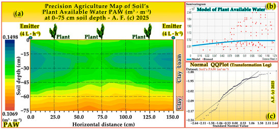
Figure 1.
(a) Precision agriculture map (N = 60) of soil PAW (m3·m−3) for 0–75 cm depth with emitters (4 L·h−1 with internal spacing 0.75 m), plants and their locations, (b) Plot of PAW semi-variogram model, and (c) Normal QQ Plot of PAW by logarithmic transformation.
As an example, the soil profile pattern of PAW (m3·m−3) is plotted in a precision agriculture profile map (Figure 1a), accompanied by a semi-variogram plot of PAW (Figure 1b) and a normal QQ Plot by log transformation (Figure 1c). In addition, the transformed parameters with the Box−Cox transformation were θsat and Ks.
The results of the granular analysis for all soils at the sites obtained the following mean values: clay (size: <0.002 mm) = 35.991 (±0.667)%, gravel = 0.080 (±0.007)% wt, sand pr (size: 0.2–2 mm) = 11.205 (±0.235)%, silt (size: 0.002–0.02 mm) = 39.218 (±0.385)%, very fine sand (size: 0.02–0.2 mm) = 13.586 (±0.163)%, and Kfactor = 0.038 (±0.001) Mg·ha·h·ha−1·MJ−1·mm−1.
In agroecosystems, the spatial diversity of soil attributes can be estimated using geostatistical analysis and modeling interpolation [2,8,16,33,95,104,106]. Ordinary kriging interpolation has proven to be the most widely implemented interpolation model for estimating the spatial layout of soil, water, and crop attribute diversity [2,16,31,33,104,108,109,110,111,112,113,114,115]. The selection of the OrKr model to be employed is driven by the properties, statistical data metrics, and the favored spatial model [16]. Therefore, the accurate estimation of these soil variables depends on the existence of spatial dependencies and correlations between the sample observed data at each site, as determined by the semi-variogram [107]. The ten PA spatial variability maps created for the 0–75 cm depth of soil’s “granular group” parameters (Figure 2a–e) revealed that clay and silt maps were similar in terms of spatial variation patterns.
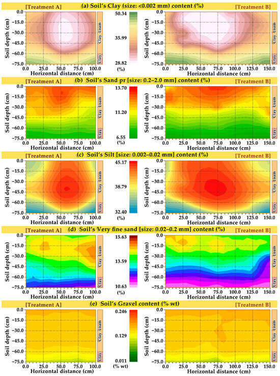
Figure 2.
Ten precision agriculture profile maps of (a) clay (size: <0.002 mm), (b) sand pr (size: 0.2–2 mm), (c) silt (size: 0.002–0.02 mm), (d) Vfs sand (size: 0.02–0.2 mm), and (e) gravel (N = 60 for each parameter).
Such spatially consistent variation is due to the fact that these soil characteristics are interrelated, and additionally, they were found to have a very strong negative correlation coefficient (rcc) [80,81] of rcc = −0.901. The interrelationship between soil granular and hydraulic properties has also been reported in other studies [2,16,79,115,116,117,118,119,120,121].
The silt (size: 0.002–0.02 mm) (%) map patterns correlation, except the outcome that presents a very strong negative correlation rcc = −0.901 (p = 0.01 (2-tailed)) only with clay (%) patterns, they present moderate positive rcc = 0.477 with sand pr (%), and weak positive rcc = 0.360 with Vfs (%), and gravel (% wt) map patterns (rcc = 0.275 (p = 0.05, 2-tailed)). In addition, the clay (%) map patterns were found to have a strong negative correlation rcc = −0.651 (p = 0.01, 2-tailed) with sand pr (%) patterns and with Vf sand (%) map patterns having rcc = −0.597 (p = 0.05, 2-tailed). The clay (%) map patterns show a weak negative correlation with gravel (% wt) (rcc = −0.241 (p = not significant)).
In addition, the sand pr (size: 0.2–2 mm) (%) map patterns presented a strong positive correlation (rcc = 0.675) with gravel patterns and a moderate positive correlation (rcc = 0.477) with silt (%) maps. Additionally, they presented a weak positive correlation (rcc = 0.375) with the Vfs (%) maps.
Vf sand (size: 0.02–0.2 mm) (%) maps (Figure 2d) except the outcome that presents a moderate negative correlation rcc = −0.597 (p = 0.01, 2-tailed) with clay (%) maps (Figure 2a), they present a strong negative correlation rcc = −0.651 with sand pr (%) maps (Figure 2b), and a weak correlation rcc = 0.360 with silt (%) maps (Figure 2c). Finally, they present a weak negative correlation rcc = −0.342 with gravel (% wt) maps (Figure 2e).
Considering that the total of the four fractions (clay, silt, sand pr, and Vf sand) of soil particles is a fixed number (100%), they are inversely related to one another, except for sand pr with Vf sand and silt. Therefore, it was expected that maps of sand pr (%), Vf sand (%), and silt (%) would be negatively correlated with clay (%) map patterns (Figure 2a). PA soil maps generated for the “granular group” features revealed that the maps of the clay (Figure 2a) and silt fractions (Figure 2c) were very similar in terms of spatial variation patterns, with a negative correlation among all sites and treatments. This consistent spatial variation is because these two soil characteristics are closely related in nature and show a very strong negative correlation (rcc = −0.901 (p = 0.01, 2-tailed).
Furthermore, the spatial variability of sand pr and Vf sand maps was in contrast to the variability of the clay fraction maps, given their reversed nature, with an enhancement of one lowering the content of the other. Similarly, the modeled variation PA maps of granular attributes revealed that the maps of Vf sand in Figure 2d had similar spatial variation patterns with the sand pr map patterns (Figure 2b) associated with each other with a weak correlation of rcc = 0.375 (p = 0.01, 2-tailed).
The outcomes of the hydraulic attribute analysis of the soils of the sites obtained the following mean values: θfc = 38.119 (±0.274)% vol., θwp = 24.011 (±0.209)% vol., θsat = 49.436 (±0.755)% vol., PAW = 0.1351 (±0.0014) m3·m−3, and BD = 1.396 (±0.019) g·cm−3. The θsat (% vol.) map patterns (Figure 3a) at p = 0.01 level (2-tailed) except the outcome that presents significant very strong correlation rcc = 0.809 with θfc (% vol.) maps (Figure 3b), and a strong correlation (rcc = 0.682) with Ks (10−3·cm·s−1) and BD (g·cm−3) maps (rcc = −0.685), they present a moderate correlation rcc = 0.574 with θwp (% vol.) maps, and a weak correlation rcc = 0.387 with PAW (m3·m−3) maps. The θfc (% vol.) map patterns (Figure 3b) present a significant, very strong correlation rcc = 0.907 with θwp maps (Figure 3c). Additionally, θfc (% vol.) maps present a very strong correlation rcc = 0.809 with θsat maps (Figure 3a), and a moderate negative correlation rcc = −0.585 with soil BD (g·cm−3) maps (Figure 3d).
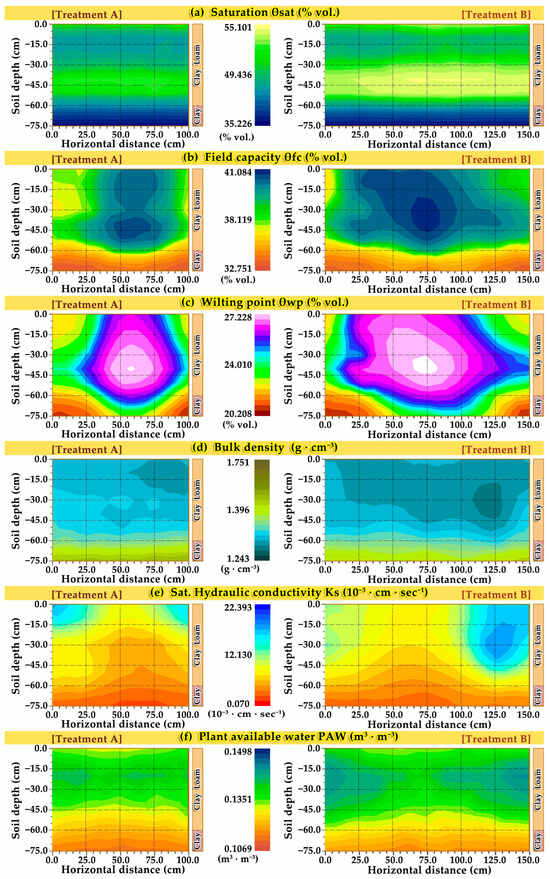
Figure 3.
Twelve precision agriculture profile maps (A and B sites) of soil: (a) saturation θsat; (b) field capacity θfc; (c) wilting point θwp; (d) bulk density BD; (e) Sat. hydraulic conductivity Ks, and (f) plant available water PAW (N = 60 for each parameter).
The θwp (% vol.) map patterns (Figure 3c) present significant strong correlation rcc = 0.907 with θfc (% vol.) maps (Figure 3b). Additionally, they presented a moderate correlation (rcc = 0.574) with θsat (% vol.) maps (Figure 3a). The PAW (m3·m−3) map patterns in Figure 3f present a very strong correlation rcc = 0.816 with Ks (10−3·cm·s−1) maps (Figure 3e) and a strong negative rcc = −0.777 with BD (g·cm−3) map patterns (Figure 3d). The BD (g·cm−3) map patterns (Figure 3d) presented strong negative correlations (rcc = −0.685, and rcc = −0.697) with θsat (% vol.), and Ks (10−3·cm·s−1) maps (Figure 3a,e), respectively. In addition, the BD (g·cm−3) maps present a moderate negative correlation rcc = −0.585 with θfc (% vol.) maps.
The generated twelve PA variability maps of the “hydraulic group” parameters (Figure 3a–f) revealed that the θfc and θwp maps were similar in their spatial variation patterns. The generated maps of field capacity θfc (Figure 3b) depicted highly congruent spatial variation patterns with wilting point θwp (Figure 3c) maps (rcc = 0.907 (p = 0.01, 2-tailed).
The developed maps of PAW (Figure 3f) showed a congruent positive variation pattern to Ks maps (Figure 3e) with rcc = 0.816 (p = 0.01, 2-tailed) and a negative pattern with BD maps in Figure 3d (rcc = −0.777). Soil hydraulic properties are intrinsically interrelated, and similar results have been reported in other studies [2,16,79,115,116,117,118,119,120,121]. The generated twenty-two PA rootzone profile maps of the soil’s hydraulic and textural parameters visualize the spatial variation of these variables and could be potentially applied to site-specific TDR sensor measurements and management zones (MZ) in precision agriculture.
3.4. Sensors Measurements of Rootzone SWC Using Various Calibration Methods in Clay Loam and Clay Soils
The variation coefficient of gravimetric soil-core water content θvg (m3·m−3) was classified as moderate CV for clay loam and clay soils, except for clay soils in site B, where it was classified as low CV. The gravimetric soil-core water content θvg (m3·m−3) in clay loam soils varied from 0.1087 to 0.4035 m3·m−3 (mean θvg = 0.2566 m3·m−3 in combined treatments A and B of all experimental sites), and the soil-core water content θvg (m3·m−3) in clay soils varied from 0.1115 to 0.3251 m3·m−3 with a mean of clay soils a θvg = 0.2739 m3·m−3 in combined treatments A and B.
The TDR sensor field measurements of SWC –M1 (m3·m−3) according to factory [67] in clay loam soils varied from 0.1393 to 0.4600 m3·m−3 (mean = 0.3102 m3·m−3 in treatments A and B), and the (m3·m−3) using sensors calibration M1 [67] in clay soils varied from 0.2057 to 0.3910 m3·m−3 (mean = 0.3424 m3·m−3). The CV of sensors measurements SWC (m3·m−3) using sensors calibration M1 [67] was classified as moderate for clay loam and clay soils, except for clay soils in site B where it was classified as low CV.
The TDR sensor measurements of soil water content (m3·m−3) using calibration method 2 [73] of time domain reflectometry sensors in clay loam soils varied from 0.1299 to 0.4236 m3·m−3 (mean = 0.2864 m3·m−3 in combined treatments A and B), and the (m3·m−3) using sensors calibration method 2 of [73] in clay soils varied from 0.1907 to 0.3604 m3·m−3, with mean = 0.3159 m3·m−3 in combined treatments A and B of all experimental sites.
The variation coefficient of TDR sensors measurements SWC (m3·m−3) using sensors calibration method 2 [73], was classified as moderate for clay loam and clay soils except for clay soils in site B and for clay soils in combined treatments A and B, where it was classified as low CV. In Table 2, descriptive statistics of gravimetric soil-core θvg (m3·m−3), and sensors SWC (m3·m−3) using M1 and M2 are presented.
Table 2.
Descriptive statistics of gravimetric soil-core θvg (m3·m−3), and sensors SWC (m3·m−3) using M1 and M2.
Moreover, in Figure 4, representative diagrams for sensor calibration method 2 [73] of the 1st experimental week for treatments A and B are presented. In Figure 4a,b are presented diagrams of the TDR sensors corrected time delay (ns) versus soil-core water content θvg (m3·m−3) with linear regression analysis for the relationship between θvg (m3·m−3) and TDR sensors corrected time delay (ns) for clay loam, clay, and all soils (combined CL and C soils). The proportion of the variation in the soil-core water content θvg that is predictable from the TDR sensors corrected time delay for all soils, resulting in high for both treatments. The coefficients of determination for all soils in treatments A and B were R2A = 0.965 and R2B = 0.983, respectively.
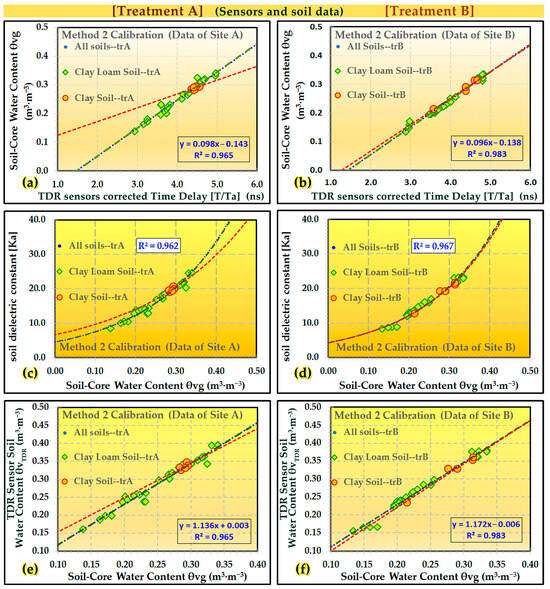
Figure 4.
Representative diagrams of treatments A and B for sensor calibration method 2 (N = 60 for each parameter) in the 1st experimental week: (a,b) TDR sensors corrected time delay vs. soil-core θvg, (c,d) θvg vs. soil dielectric constant Ka, (e,f) θvg vs. TDR sensors SWC θvTDR.
The regression dashed lines for CL and C soils are shown in Figure 4a,b to highlight the variations in slope and intercept between the soil textures and treatments. In tr. A (site A), there was a significant slope difference between the CL and C soils, while in tr. B (site B), there was no significant slope difference between the CL and C soils, which is probably due to the differences in hydraulic parameters between the sites and because in tr. B, there was a greater degree of scatter in the data in clay soils than in tr. A (Figure 4a,b). Significant slope differences between sites have also been reported in other studies [114,115].
In Figure 4c,d representative diagrams of soil-core water content θvg (m3·m−3) versus soil dielectric constant Ka are depicted for the 1st experimental week. The exponential regression dashed lines for CL and C soils are shown in Figure 4c,d to highlight the variations in slope and intercept between soil textures and treatments. In both Figure 4c,d, the Ka values compare well with the measured θvg. The proportion of the variation in the soil dielectric Ka that was predictable from the θvg (m3·m−3) for all soils in treatments A and B was high for both treatments. The R-squared values for all soils in treatments A and B were R2A = 0.962 and R2B = 0.967, respectively. In Figure 4e,f, diagrams of θvg (m3·m−3) versus TDR sensors SWC –M2 are presented, with linear regression analysis for the relationship between SWC θvg, and TDR sensors SWC –M2 (m3·m−3) for CL and C soils. The regression dashed lines for CL and C soils are shown in Figure 4e,f to illustrate the differences in slope and intercept between soil textures and treatments. In both Figure 4e,f, the TDR sensors SWC –M2 values using M2 [73], compare well with the measured SWC θvg. The proportion of the variation in the TDR sensors SWC –M2 that is predictable from the SWC θvg for all soils resulted as high for both treatments.
The coefficients of determination for all soils in treatments A and B were R2A = 0.965 and R2B = 0.983, respectively. In tr. There was a significant slope difference between the CL and C soils, while in tr. B, there is no significant slope difference between CL and C soils, which is probably due to the differences in hydraulic parameters between sites and because in tr. B, there was a higher degree of dispersion in the data for C soils than for tr. A. Significant slope differences between sites have also been reported in other studies [114,115].
In Figure 5a,b, dynamic diagrams of treatments A and B are depicted, with spatiotemporal changes in soil moisture over time of the experiment at different soil depths and textures for sensor calibration methods 1 [67] and 2 [73], to demonstrate the spatiotemporal distribution patterns of SWCs in the traditional way. There are many differences between the spatiotemporal distribution patterns and measurement values of SWCs at different soil depths. in treatments A and B (Figure 5a,b), between method 1 [67] and method 2 [73] of the time domain reflectometry sensor calibration methods, and between the textures of clay loam and clay soils.
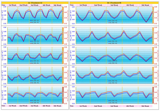
Figure 5.
Dynamic diagrams of moisture (N = 60 for each parameter in every experimental week) spatiotemporal changes over time, at different soil depths and textures for sensor calibration methods M1 and M2, of (a) treatment A and (b) treatment B.
These differences in spatiotemporal distribution patterns and SWCs field measurement values of the TDR sensors are easier to observe and understand by scientists. In contrast, for farmers, it is more difficult to identify these spatiotemporal patterns and discrete differences in soil moisture measurement values of the TDR sensors, understand their differences, and use these plots for their farm input and output management and for proper environmental irrigation decisions. The above are the main reasons that motivated us to establish a new geostatistical approach to generate and visualize the spatiotemporal distribution patterns and sensors’ measurement values of root zone moisture profiles and their changes over the time of the experiment on precision agriculture soil moisture profile SWC –M1 (m3·m−3) and SWC –M2 (m3·m−3) maps, in order to provide a new approach that will help scientists and, more importantly, farmers to understand more easily and clearly the dynamics of moisture in the root zone of crops in order to make appropriate and timely environmental irrigation decisions.
3.5. Validation Statistical Measures and Percentage Differences of TDR Sensors SWC (m3·m−3) Versus Gravimetric θvg (m3·m−3), of Various Sensors Calibration Methods
Table 3 presents all the results of the validation statistical measures for the different calibration methods of the TDR sensors (M1 [67] and M2 [73]) under sugarbeet field conditions (Treatments A and B) in sites A and B with various soil textures. Estimates of sensors (m3·m−3) obtained for CL and C soils using the sensors calibration M2 method [73] were compared with field soil-core observations resulting in RMSE values ranging from 0.0373 to 0.0395 m3·m−3 for CL soils and from 0.0405 to 0.0455 m3·m−3 for C soils. The RMSE values obtained for the TDR sensor calibration M2 method [73] were within the values 0.0326 to 0.0581 m3·m−3 found in other studies [2,114].
Table 3.
Validation of statistical measures of TDR sensors field measurements results of SWC using different calibration methods (M1 & M2) in various soil textures.
Moreover, the accuracy of TDR sensor field measurement values is very important in conjunction with actual irrigation scenarios for each site and soil texture. In our study, using TDR sensors calibration method 2 [73] versus factory calibration method 1 [67] for actual irrigation scenarios, it resulted in a better mean 9.34% (9.45% for site A and 9.23% for site B) difference between sensors SWC –M2 (m3·m−3) and sensors SWC –M1 (m3·m−3) field measurement values, in conjunction with the actual soil moisture values, that is, the gravimetric soil-core SWC θvg (m3·m−3) values in each site.
This means that in actual irrigation scenarios, in order to make an informed and appropriate irrigation decision, using SWC –M2 (m3·m−3) values compared to the higher values found for SWC –M1 (m3·m−3) would be 9.34% closer to the actual gravimetric SWC content θvg (m3·m−3) values of the soil’s root zone profile.
Using the higher SWC –M1 (m3·m−3) values for an irrigation decision would have delayed the actual crop irrigation compared to the lower and more accurate SWC –M2 (m3·m−3) values that resulted in the two treatments for all soils in an average 9.34% (with a mean of 9.24% for CL soils and a mean of 15.58% for C soils) difference closer to the actual soil moisture values of the gravimetric soil-core SWC θvg (m3·m−3).
Therefore, the results of the sensor field measurement values using the calibration method M2 are more valuable in environmental irrigation decision-making for a more accurate and timely decision on actual crop irrigation.
3.6. Exploratory Data Analysis and Precision Agriculture Geostatistical Modeling of TDR Sensors Measurements of Rootzone SWC Using Various Sensors Calibration Methods
Prior to the geostatistical analysis, an exploratory data analysis was conducted, as modeling of TDR sensors measurements of rootzone soil water content ) under sugarbeet field conditions using various methods of TDR sensor calibration. Two significant statistical indicators of the tested soil moisture in the experimental plots are skewness and kurtosis [87,88,104]. The statistical measure of skewness resulted in a positive (right-tailed skewness) 0.005 for the (m3·m−3) of 3rd week measurements. On the contrary, skewness varied negatively (left-tailed skewness) from −0.195 to −0.019 for the following soil moisture measurements (in ascending order): (m3·m−3) of 1st, 2nd, 4th, and 5th week of experiment. After the assessment of skewness and kurtosis, a parallel result for both statistical metrics suggested that four out of ten total parametric datasets of soil (m3·m−3), had to be subjected to transformation in order to validate that the assumption of variance equality of the data values was fulfilled and that their data points were normally allocated [2,103]. The above results show that these soil moisture datasets have an abnormal distribution [79,105,106,107,108]. Considering the above-mentioned results, these soil moisture datasets were subjected to logarithmic transformations [79,104,105,106,107,108]. The transformed parameters with logarithmic transformation were –M1 and –M2 datasets of 1st week, and –M1 and –M2 datasets of 2nd week.
3.7. Best-Fitted Models, Spatial Dependence, and Validation of Geostatistical Imaging of Soil’s Hydraulic, Granular, and SWC Datasets Using Various Sensors Calibration Methods
In order to examine and evaluate the spatial variance of the field’s soil attributes and TDR sensor SWCs, semi-variograms were calculated by applying the OrKr method of interpolation.
The generated PA maps of the soil’s granular group (Figure 2a–e), hydraulic group (Figure 3a–f), TDR sensors SWC –M1 (m3·m−3) group using calibration M1 (Figure 6a–e), and SWC –M2 (m3·m−3) group using calibration M2 (Figure 7a–e) was modeled and created using the best-fit models, which described the spatial patterns of the various soil properties and moisture contents. The PA profile map images depict the spatial and temporal SWCs variability with a very high resolution at the centimeter scale. For each of the field’s soils (granular and hydraulic) and SWC parameters, seven models were trialed, analyzed, and validated. The best-fitted models mirror the varying spatial variability induced by the nature of the soil and SWC variables, which was also associated with the prevailing environmental conditions of the field.
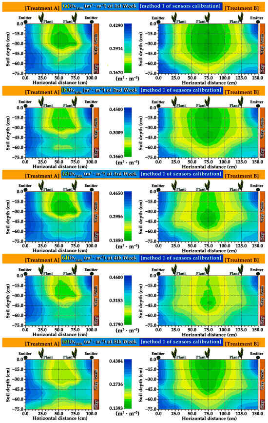
Figure 6.
Ten precision agriculture moisture profile maps created using sensor calibration M1 (factory cal. [67]) with emitters (4 L·h−1/0.75 m) and plant locations of: (a) θvTDR of the 1st week; (b) θvTDR of the 2nd week; (c) θvTDR of the 3rd week; (d) θvTDR of the 4th week, and (e) θvTDR of the 5th week (N = 60 for each parameter every week).
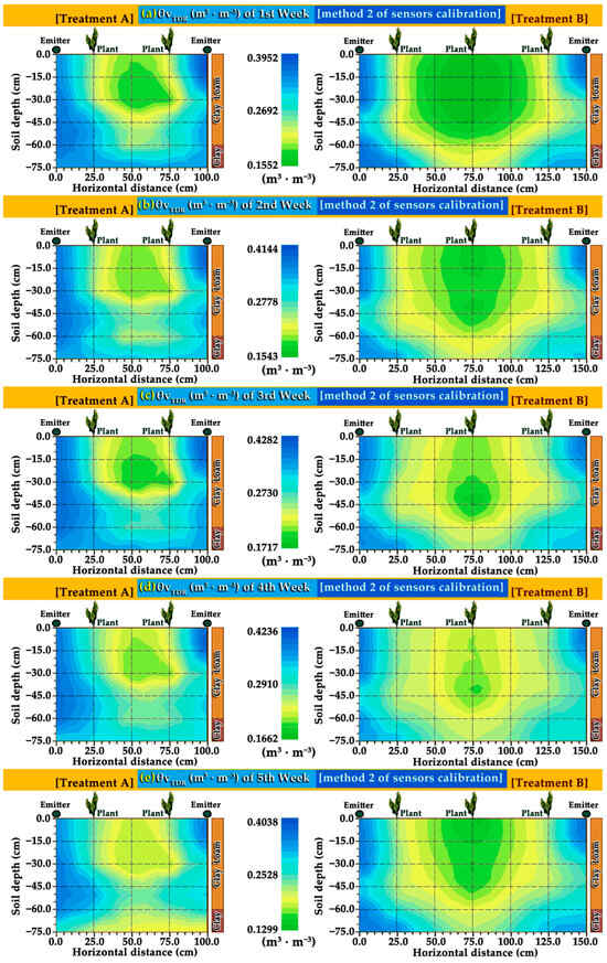
Figure 7.
Ten precision agriculture moisture profile maps generated using sensor calibration M2 (Topp & Reynolds [73]), with emitters (4 L·h−1/0.75 m) and plant locations, of: (a) θvTDR of the 1st week; (b) θvTDR of the 2nd week; (c) θvTDR of the 3rd week; (d) θvTDR of the 4th week, and (e) θvTDR of the 5th week (N = 60 for each parameter in every experimental week).
According to the modeling results, the best-fitting semi-variogram models obtained for the granular parameters were circular, exponential, pentaspherical, and spherical models. Accordingly, the best-fitting models obtained for the hydraulic parameters were the exponential, circular, and spherical models. Based on the modeling results, the best-fitting model obtained for SWC –M1 (m3·m−3) group [67] was the exponential for all experimental weeks and for the SWC –M2 (m3·m−3) group [73] were the exponential for 2nd to 5th experimental week and the spherical for the 1st week of experiments.
By studying the resulting SWC –M1 (m3·m−3) (Figure 6a–e), and SWC –M2 (m3·m−3) (Figure 7a–e) high accuracy maps of the experimental weeks, it is obvious that the soil water content does not only vary in the vertical axis (various soil layers at various depths) but also changes in the horizontal plane. Moreover, it is observed that the lowest moisture values obtained for SWC –M1 (m3·m−3) in Figure 6a–e and SWC –M2 (m3·m−3) in Figure 7a–e high accuracy maps of the experimental weeks are located in the center of the distance (and downward) between the water sources (left and right emitter) as expected and are depicted in green (dark, medium and light) colors.
The best-fitted models, percentage of the group’s best-fitted model, parameter list, nugget-to-sill ratio (N:S ratio) of each model, spatial dependence, and RRMSE modeling results are presented in Table 4.
Table 4.
Group’s parameters list the best-fitted geostatistical models, the percentage of the group’s best-fitted model (%), the model’s N:S ratio, spatial dependence, and RRMSE.
Moreover, the green patterns of the lowest soil moisture values obtained for SWC –M1 and –M2 (m3·m−3) are located mostly in the clay loam soils in both treatments and vary extensively between the experimental weeks. It is also observed that the spatial extent of the green patterns (lower soil moisture values) is smaller in tr. A because the distance between the water sources (left and right emitters) was shorter (1.0 m) than that in tr. B (1.5 m).
A remarkable outcome is that both the resulting SWC –M1 (Figure 6a–e), and SWC –M2 (Figure 7a–e) high accuracy maps present patterns of high similarities with the map patterns of the wilting point θwp (% vol.) maps in Figure 3c (p < 0.001) in all experimental weeks, having strong negative correlations in 1st through 4th week (rcc (1st week) = −0.739, rcc(2nd week) = −0.712, rcc(3rd week) = −0.659, rcc(4th week) = −0.649), and moderate negative correlation in 5th week (rcc(5th week) = −0.527).
Another important outcome is that both the SWC –M1 (Figure 6a–e) and SWC –M2 (Figure 7a–e) high accuracy maps present patterns of high similarities (p < 0.001) with the patterns of the θfc (% vol.) maps (Figure 3b), having strong negative correlations in 1st through 4th week (rcc(1st week) = −0.652, rcc(2st week) = −0.620, rcc(3rd week) = −0.617, rcc (4th week) = −0.622), and moderate negative correlation in 5th week (rcc(5th week) = −0.426). The SWC’s –M1 (and SWC’s –M2 high accuracy maps (Figure 6 and Figure 7) present high and medium similarities (p < 0.001) with the patterns of silt (%) maps (Figure 2c), in all experimental weeks, having strong and moderate negative correlations (rcc(1st week) = −0.729 to rcc(5th week) = −0.417). Additionally, SWC –M1 and SWC –M2 high accuracy maps present patterns of high and medium similarities (p < 0.001) with patterns of clay (%) maps, in 1st through 4th week, having strong correlations (rcc(1st week) = 0.627 to rcc(4th week) = 0.594), and moderate correlation in the 5th week (rcc(5th week) = 0.449). Soil granular and hydraulic properties are intrinsically interrelated [2,16,79,115,116,117,118,119,120,121]. Other studies [2,6,117,121] have also found strong positive correlations between SWC and clay content in the 0–100 cm soil layers [117,121] and in 0–75 cm soil layers [2,6].
The SWC –M1 and SWC –M2 (m3·m−3) high accuracy maps present patterns of negative similarities with the patterns of the sand pr (%) maps (Figure 2b), having negative correlations of rcc(1st week) = −0.237 to rcc(4th week) = −0.200, and (rcc(5th week) = −0.098). Other studies have also found negative correlations between SWC and sand content in the 0–75 cm [2,6] and 0–100 cm [117,121] soil layers. In SWC –M1 (m3·m−3) group using sensors calibration M1 [67], the maps (Figure 6a–e) of 1st through 5th week resulted in strong spatial dependence. In SWC –M2 (m3·m−3) group using sensors calibration M2 [73], the maps (Figure 7a–e) of all weeks, resulted also in strong spatial dependence.
We recommend method M2 for sensor calibration because it was found to be more accurate, with the lowest statistical and geostatistical validation errors, and the best validation measures for accurate soil moisture profile maps, which were obtained for clay loam soils over clay soils. In the granular group (Figure 2a–e), the clay (%), Vf sand (%), sand pr (%), and silt (%) maps resulted in strong spatial dependence, while only the gravel (% wt) maps presented a weak spatial dependence. In the hydraulic group (Figure 3a–e), the θfc (Figure 3b) and θwp maps (Figure 3c) resulted in a strong spatial dependence. The BD (g·cm−3) and Ks (10−3·cm·s−1) maps (Figure 3d,e) resulted in medium spatial dependence, while the θsat (% vol.) and PAW (m3·m−3) maps showed weak spatial dependence. The outcomes of soil and parameters, best-fitted geostatistical models for rootzone 2D SWCs mapping, and validation geostatistical measures [En-s (Nash-Sutcliffe model efficiency), MPE, RMSE, MSPE, RMSSE, ASE, and MSDR] are presented in Table 5.
Table 5.
Results of soil and parameters, best-fitted geostatistical models for rootzone 2D mapping, and various validation geostatistical measures with bold text indicating the best values.
The En-s or NSE [90] ranges from −∞ to 1.0 (NSE = 1.0 is the optimal value suggesting perfect model fit), while efficiency values between 0.0 and 1.0 are widely regarded as accepted levels for model performance. Efficiency values less than 0.0 indicate that the observable average is a better predictor than the modeled value [92]. In the granular group, the validation geostatistical measure En-s [90,91,92,113] was classified as “well” [2,91] for the circular geostatistical model applied for 2D mapping of clay (%) maps (Figure 2a).
The validation geostatistical measure En-s (NSE) [90,91,92,113] was classified as “satisfying” [2,91] for the pentaspherical geostatistical model (Table 5) applied for silt (%) 2D maps (Figure 2c) and for sand pr (%) 2D maps (Figure 2b). In contrast, the En-s model efficiency [90,91,92,113] was classified as “less satisfactory” [2,91] for the exponential model applied to the very fine sand (%) 2D maps (Figure 2d) and for the spherical geostatistical model applied to the gravel (% wt) 2D maps (Figure 2e).
In hydraulic group, the En-s (NSE) model efficiency [90,91,113] was classified as “well” [2,91] for the exponential geostatistical model applied for 2D mapping of the θsat (% vol.) 2D maps (Figure 3a), as “satisfying” [2,91] for the spherical model applied for the θwp (% vol.) 2D maps (Figure 3c), and also for the exponential model applied for the field capacity θfc (% vol.) 2D maps (Figure 3b). In contrast, the En-s [90,91,113] model efficiency was classified as “less satisfactory” [2,91] for the circular model applied to the PAW (m3·m−3) 2D maps (Figure 3f), as well as for the exponential model applied to the bulk density (g·cm−3) 2D maps (Figure 3d) and Ks (10−3·cm·s−1) 2D maps (Figure 3e). In SWC –M1 (m3·m−3) group using sensors calibration method 1 [67], the NSE was classified as “satisfying” [2,91] for the exponential geostatistical model applied for the –M1 (m3·m−3) of 1st through 5th week 2D maps (Figure 6a–e).
In SWC –M2 (m3·m−3) group using sensors calibration M2 [73], the NSE was classified as “satisfying” [2,91] for the spherical model applied on 1st week 2D maps (Figure 7a), and also for the exponential model applied on 2nd through 5th week 2D maps (Figure 7b–e). The NSE model efficiency values for SWC (m3·m−3) using calibrations M1 [67] and M2 [73] were found to be 0.5383 to 0.6501 for M1 and 0.5379 to 0.6657 for M2, respectively. Our above NSE validation values are within the NSE values of 0.42 to 0.87 found in other research studies for soil moisture validation [2,91].
In the granular group, the best values were MPE = 0.00233, RMSE = 0.0583, and ASE = 0.0797 for the 2D maps of gravel (% wt) (Figure 2e). The best MSPE and RMSSE errors were found for silt (%) (Figure 2c) and clay (%) 2D maps (Figure 2a), respectively. In another study regarding soil texture [115], the reported kriging’s RMSE error values for sand, silt, and clay were 3.25, 3.16, and 0.67, respectively, which compare well with our RMSE values of 0.9739, 1.5290, and 2.3067. In the hydraulic group, the best MPE, RMSE, MSPE, and ASE errors resulted for the PAW (m3·m−3) 2D maps (Figure 3f), and the best RMSSE error was found for the saturation θsat (% vol.) 2D maps (Figure 3a).
In SWC –M1 (m3·m−3) group using sensors calibration method M1 [67], the best MPE, MSPE and ASE errors resulted for –M1 (m3·m−3) of 5th week 2D maps (Figure 6e), and the best RMSE and RMSSE resulted for –M1 (m3·m−3) of 4th week 2D maps (Figure 6d). In SWC –M2 (m3·m−3) group using calibration method M2 [73], the best MPE and MSPE errors resulted for –M2 (m3·m−3) of 5th week 2D maps (Figure 7e), the best RMSSE resulted for –M2 (m3·m−3) of 4th week 2D maps (Figure 7d), and the best RMSE and ASE resulted for –M2 (m3·m−3) of 1st week 2D maps (Figure 7a).
In the granular group, the best MSDR values of 0.9455 and 0.6817 were obtained for the pentaspherical and exponential geostatistical models applied to the sand (%) (Figure 2b) and silt (%) 2D maps (Figure 2c), respectively. In the hydraulic group, the best MSDR values of 1.2252 and 1.5763 resulted from the exponential model applied to the 2D maps (Figure 3e) of Ks (10−3·cm·s−1) and BD (g·cm−3) 2D maps (Figure 3d), respectively.
In the SWC –M1 (m3·m−3) group using sensors calibration M1 [67], the best MSDRs 0.9695 and 0.9183 resulted in the exponential model applied for the SWC –M1 (m3·m−3) of 3rd week (Figure 6c), and of 4th week 2D maps (Figure 6d), respectively. In SWC –M2 (m3·m−3) group using sensors calibration M2 [73], the best MSDRs 0.9691 and 0.9182 resulted in the exponential model applied for the SWC –M2 (m3·m−3) of 3rd week 2D maps (Figure 7c) and 4th week 2D maps (Figure 7d), respectively. Regarding the validation geostatistical measures of the granular group, hydraulic group, SWC –M1 (m3·m−3) group using M1 [67], and SWC –M2 (m3·m−3) group using M2 [73], the best results for the parametric 2D maps depend on the dataset structure and features and on the mathematical nature of the particular geostatistical measures used.
Most of the time, it is difficult to finalize only one parameter with the best results of the validation geostatistical measures. There is much debate on the best validation geostatistical measure [1,2,6,16,31,33,74,75,76,77,78,79,80,86,87,88,89,90,91,92,102,103,104,105,106,107,113]. The results of the mean MPE, MSPE, and ASE errors are all around 0.0, as expected, and we can consider them approximately the same. The average RMSE errors are short but with distinguishing differences (especially in the cases of the models applied for SWC –M1 and –M2 (m3·m−3) of 1st through 5th week 2D maps) within each dataset of weekly data; they are clearly worse (larger) for the –M1 subsets. The major differences were found in the RMSE and RMSSE errors, the En-s (NSE) model efficiency, and the MSDR. Based on these criteria, the pentaspherical and exponential geostatistical models are recommended for the kriging and spatial mapping of soil granular parameters, and the exponential and spherical geostatistical models are recommended for the kriging and spatial mapping of soil hydraulic parameters.
As for soil moisture, the exponential and spherical geostatistical models are those that we recommend use for kriging, spatial and temporal mapping for SWC –M1 (m3·m−3) when sensors calibration method M1 according to factory [67] is applied, and for SWC –M2 (m3·m−3) when sensors calibration method M2 [73] is applied.
Moreover, the SWC –M2 (m3·m−3) was found to be more accurate than SWC –M1 (m3·m−3) with the lowest statistical and geostatistical errors and best validation measures in clay loam soils and clay soils. The best validation measures for SWC (m3·m−3) were obtained for clay loam soils compared to those of clay soils, indicating that field sensor measurements, geostatistical modeling, and mapping of SWC (m3·m−3) is more accurate in clay loam soils. In the SWC –M1 (m3·m−3) and SWC –M2 (m3·m−3) geostatistical maps in Figure 6a–e and Figure 7a–e, we can observe minimum changes in SWCs measured by TDR sensors from experimental week one to five in treatment A (site A), but they are observed much higher changes in soil water contents measured by TDR sensors in treatment B (site B). Visualizing these SWCs results via geostatistical maps of soil root zone profiles (2D maps) assists farmers and scientists in making informed, better, and timely environmental irrigation decisions and optimizing energy, saving irrigation water, increasing water-use efficiency and crop production, reducing crop costs, and managing water resources sustainably.
Regarding the study limitations, the number of soil samples could be a difficult task in field sampling labor and the economic cost of soil laboratory analyses for some farmers.
4. Conclusions
The precise measuring and knowledge of the spatiotemporal distribution of SWC (m3·m−3) is crucial in many sectors of both environment and agronomy. Modeling results revealed that for granular parameters, the best-fitted semi-variogram models were circular, exponential, pentaspherical, and spherical, and for the hydraulic parameters, they were exponential, circular, and spherical. Regarding the SWC –M1 using sensors calibration M1 (factory calibration), the best-fit model was the exponential, and for the SWC –M2 using sensors calibration M2 were the exponential and spherical models.
The resulting best geostatistical validation measures of precision agriculture profile SWC (m3·m−3) maps found were Nash-Sutcliffe model efficiency NSE = 0.6657, MPE = 0.00013, RMSE = 0.0385, MSPE = −0.0022, RMSSE = 1.6907, ASE = 0.0418, and MSDR = 0.9695. The exponential and spherical models were found to be the best for kriging and spatial mapping for profile SWC (m3·m−3) 2D maps and sensors calibration M2 were found to be more accurate with the lowest statistical and geostatistical errors, and the best validation measures were obtained for CL soils compared to those for C soils. Using the higher SWC –M1 (m3·m−3) values for an irrigation decision would have delayed the actual crop irrigation compared to the lower and more accurate SWC –M2 (m3·m−3) values that resulted for both treatments in an average of 9.34% (with a mean of 9.24% for CL soils and mean of 15.58% for C soils) difference closer to the actual SWC θvg (m3·m−3) gravimetric values. Therefore, the results of the sensor field measurement values using calibration M2 are more valuable in environmental irrigation decision-making for a more accurate and timely decision on actual crop irrigation.
Visualizing the SWC results and their temporal changes via geostatistical 2D maps of soil root zone profiles assists farmers and scientists in making informed, better, and timely environmental irrigation decisions and optimizing energy, saving irrigation water, increasing water-use efficiency and crop production, reducing crop costs, and managing water resources sustainably. In the future, there will be a growing necessity for accurate maps displaying spatio–temporal profiles of soil water content sensor information to enhance spatial moisture analysis and interpretation to assist scientists and farmers in making informed, better, and appropriate environmental irrigation decisions.
Future research directions for further optimization of moisture prediction models and maps include the use of machine learning algorithms (linear regression, KNN algorithm, K-means algorithm, Random Forest algorithm, SVM (Support Vector Machine) algorithm, factor analysis, etc.), genetic algorithms, fuzzy logic algorithms, and artificial intelligence.
Funding
This research received no external funding.
Data Availability Statement
The original contributions presented in this study are included in the article. Further inquiries can be directed to the corresponding author.
Conflicts of Interest
The author declares no conflicts of interest.
References
- Stamatis, G.; Parpodis, K.; Filintas, A.; Zagana, E. Groundwater quality, nitrate pollution and irrigation environmental management in the Neogene sediments of an agricultural region in central Thessaly (Greece). Environ. Earth Sci. 2011, 64, 1081–1105. [Google Scholar] [CrossRef]
- Filintas, A. Land Use Evaluation and Environmental Management of Biowastes, for Irrigation with Processed Wastewaters and Application of Bio-Sludge with Agricultural Machinery, for Improvement-Fertilization of Soils and Crops, with the Use of GIS-Remote Sensing, Precision Agriculture and Multicriteria Analysis. Ph.D. Thesis, University of the Aegean, Mitilini, Greece, 2011. [Google Scholar]
- Dymond, S.F.; Bradford, J.B.; Bolstad, P.V.; Kolka, R.K.; Sebestyen, S.D.; DeSutter, T.M. Topographic, edaphic, and vegetative controls on plant available water. Ecohydrology 2017, 10, e1897. [Google Scholar] [CrossRef]
- Liu, X.; Lai, Q.; Yin, S.; Bao, Y.; Qing, S.; Bayarsaikhan, S.; Bu, L.; Mei, L.; Li, Z.; Niu, J.; et al. Exploring grassland ecosystem water use effiency using indicators of precipitation and soil moisture across the Mongolian Plateau. Ecol. Indic. 2022, 142, 109207. [Google Scholar] [CrossRef]
- Earles, J.M.; Stevens, J.T.; Sperling, O.; Orozco, J.; North, M.P.; Zwieniecki, M.A. Extreme mid-winter drought weakens tree hydraulic–carbohydrate systems and slows growth. New Phytol. 2018, 219, 89–97. [Google Scholar] [CrossRef]
- Filintas, A. Soil Moisture Depletion Modelling Using a TDR Multi-Sensor System, GIS, Soil Analyzes, Precision Agriculture and Remote Sensing on Maize for Improved Irrigation-Fertilization Decisions. Eng. Proc. 2021, 9, 36. [Google Scholar] [CrossRef]
- Raczka, N.C.; Carrara, J.E.; Brzostek, E.R. Plant–microbial responses to reduced precipitation depend on tree species in a temperate forest. Glob. Change Biol. 2022, 28, 5820–5830. [Google Scholar] [CrossRef]
- Filintas, A.; Nteskou, A.; Kourgialas, N.; Gougoulias, N.; Hatzichristou, E. A Comparison between Variable Deficit Irrigation and Farmers’ Irrigation Practices under Three Fertilization Levels in Cotton Yield (Gossypium hirsutum L.) Using Precision Agriculture, Remote Sensing, Soil Analyses, and Crop Growth Modeling. Water 2022, 14, 2654. [Google Scholar] [CrossRef]
- Adams, P.W.; Flint, A.L.; Fredriksen, R.L. Long-term patterns in soil moisture and revegetation after a clearcut of a Douglas-fir forest in Oregon. For. Ecol. Manag. 1991, 41, 249–263. [Google Scholar] [CrossRef]
- Rodriguez-Iturbe, I.; D’Odorico, P.; Porporato, A.; Ridolfi, L. On the spatial and temporal links between vegetation, climate, and soil moisture. Water Resour. Res. 1999, 35, 3709–3722. [Google Scholar] [CrossRef]
- Detto, M.; Montaldo, N.; Albertson, J.D.; Mancini, M.; Katul, G. Soil moisture and vegetation controls on evapotranspiration in a heterogeneous Mediterranean ecosystem on Sardinia, Italy. Water Resour. Res. 2006, 42, W08419. [Google Scholar] [CrossRef]
- Tromp-van Meerveld, H.J.; McDonnell, J.J. On the interrelations between topography, soil depth, soil moisture, transpiration rates and species distribution at the hillslope scale. Adv. Water Resour. 2006, 29, 293–310. [Google Scholar] [CrossRef]
- Troch, P.A.; Martinez, G.F.; Pauwels, V.R.N.; Durcik, M.; Sivapalan, M.; Harman, C.; Brooks, P.D.; Gupta, H.; Huxman, T. Climate and vegetation water use efficiency at catchment scales. Hydrol. Process. 2009, 23, 2409–2414. [Google Scholar] [CrossRef]
- Breshears, D.B.; Myers, O.B.; Barnes, F.J. Horizontal heterogeneity in the frequency of plant-available water with woodland intercanopy-canopy vegetation patch type rivals that occurring vertically by soil depth. Ecohydrology 2009, 2, 503–519. [Google Scholar] [CrossRef]
- Cavanaugh, M.L.; Kurc, S.A.; Scott, R.L. Evapotranspiration partitioning in semiarid shrubland ecosystems: A two-site evaluation of soil moisture control on transpiration. Ecohydrology 2011, 4, 671–681. [Google Scholar] [CrossRef]
- Filintas, A.; Gougoulias, N.; Kourgialas, N.; Hatzichristou, E. Management Soil Zones, Irrigation, and Fertigation Effects on Yield and Oil Content of Coriandrum sativum L. Using Precision Agriculture with Fuzzy k-Means Clustering. Sustainability 2023, 15, 13524. [Google Scholar] [CrossRef]
- Sala, O.E.; Lauenroth, W.K.; Parton, W.J. Long-term soil water dynamics in the shortgrass steppe. Ecology 1992, 73, 1175–1181. [Google Scholar] [CrossRef]
- Carlson, D.H.; Thurow, T.L.; Knight, R.W.; Heitschmidt, R.K. Effect of honey mesquite on the water balance of Texas Rolling Plains rangeland. J. Range Manag. 1990, 43, 491–496. [Google Scholar] [CrossRef]
- Wilcox, B.P.; Seyfried, M.S.; Breshears, D.D. The Water Balance on Rangelands. In Encyclopedia of Water Science; Stewart, B.A., Howell, T.A., Eds.; Marcel Dekker: New York, NY, USA, 2003; pp. 791–794. [Google Scholar]
- Huxman, T.E.; Wilcox, B.P.; Breshears, D.D.; Scott, R.L.; Snyder, K.A.; Small, E.E.; Hultine, K.; Pockman, W.T.; Jackson, R.B. Ecohydrological implications of woody plant encroachment. Ecology 2005, 86, 308–319. [Google Scholar] [CrossRef]
- Scott, R.L.; Huxman, T.E.; Cable, W.L.; Emmerich, W.E. Partitioning of evapotranspiration and its relation to carbon dioxide exchange in a Chihuahuan Desert shrubland. Hydrol. Process. 2006, 20, 3227–3243. [Google Scholar] [CrossRef]
- Kurc, S.A.; Small, E.E. Soil moisture variations and ecosystem-scale fluxes of water and carbon in semiarid grassland and shrubland. Water Resour. Res. 2007, 43, W06416. [Google Scholar] [CrossRef]
- Moran, M.S.; Scott, R.L.; Hamerlynck, E.P.; Green, K.N.; Emmerich, W.E.; Collins, C.D.H. Soil evaporation response to Lehmann lovegrass (Eragrostis lehmanniana) invasion in a semiarid watershed. Agric. For. Meteorol. 2009, 149, 2133–2142. [Google Scholar] [CrossRef]
- Deardorff, J.W. A parameterization of ground-surface moisture content for use in atmospheric prediction models. J. Appl. Meteorol. 1977, 16, 1182–1185. [Google Scholar] [CrossRef]
- Delworth, T.; Manabe, S. Climate variability and land surface processes. Adv. Water Resour. 1993, 16, 3–20. [Google Scholar] [CrossRef]
- Jung, M.; Reichstein, M.; Ciais, P.; Seneviratne, S.I.; Sheffield, J.; Goulden, M.L.; Bonan, B.; Cescatti, A.; Chen, J.; de Jeu, R.; et al. Recent decline in the global land evapotranspiration trend due to limited moisture supply. Nature 2010, 467, 951–954. [Google Scholar] [CrossRef]
- Mittelbach, H.; Lehner, I.; Seneviratne, S.I. Comparison of four soil moisture sensor types under field conditions in Switzerland. J. Hydrol. 2012, 430–431, 39–49. [Google Scholar] [CrossRef]
- Koutseris, E.; Filintas, A.; Dioudis, P. Antiflooding prevention, protection, strategic environmental planning of aquatic resources and water purification: The case of Thessalian basin, in Greece. Desalination 2010, 250, 318–322. [Google Scholar] [CrossRef]
- Scott, R.L. Using watershed water balance to evaluate the accuracy of eddy covariance evaporation measurements for three semiarid ecosystems. Agric. For. Meteorol. 2010, 150, 219–225. [Google Scholar] [CrossRef]
- Garten, C.T., Jr.; Classen, A.T.; Norby, R.J. Soil moisture surpasses elevated CO2 and temperature as a control on soil carbon dynamics in a multi-factor climate change experiment. Plant. Soil. 2009, 319, 85–94. [Google Scholar] [CrossRef]
- Dioudis, P.; Filintas, A.; Koutseris, E. GPS and GIS based N-mapping of agricultural fields’ spatial variability as a tool for non-polluting fertilization by drip irrigation. Int. J. Sus. Dev. Plann. 2009, 4, 210–225. [Google Scholar] [CrossRef]
- Holsten, A.; Vetter, T.; Vohland, K.; Krysanova, V. Impact of climate change on soil moisture dynamics in Brandenburg with a focus on nature conservation areas. Ecol. Model. 2009, 220, 2076–2087. [Google Scholar] [CrossRef]
- Filintas, A.; Dioudis, P.; Prochaska, C. GIS modeling of the impact of drip irrigation, of water quality and of soil’s available water capacity on Zea mays L., biomass yield and its biofuel potential. Desalination Water Treat. 2010, 13, 303–319. [Google Scholar] [CrossRef]
- Falloon, P.; Jones, C.D.; Ades, M.; Paul, K. Direct soil moisture controls of future global soil carbon changes: An important source of uncertainty. Glob. Biogeochem. Cycles 2011, 25, GB3010. [Google Scholar] [CrossRef]
- Filintas, A.; Wogiatzi, E.; Gougoulias, N. Rainfed cultivation with supplemental irrigation modelling on seed yield and oil of Coriandrum sativum L. using precision agriculture and GIS moisture mapping. Water Supply 2021, 21, 2569–2582. [Google Scholar] [CrossRef]
- Broedel, E.; Tomasella, J.; Cândido, L.A.; Randow, C. Deep soil water dynamics in an undisturbed primary forest in central mazonia: Diffrences between normal years and the 2005 drought. Hydrol. Process. 2017, 31, 1749–1759. [Google Scholar] [CrossRef]
- Rigden, A.J.; Salvucci, G.D.; Entekhabi, D.; Short Gianotti, D.J. Partitioning evapotranspiration over the continental United States using weather station data. Geophys. Res. Lett. 2018, 45, 9605–9613. [Google Scholar] [CrossRef]
- Jiao, L.; An, W.; Li, Z.; Gao, G.; Wang, C. Regional variation in soil water and vegetation characteristics in the Chinese Loess Plateau. Ecol. Indic. 2020, 115, 106399. [Google Scholar] [CrossRef]
- Filintas, A.; Nteskou, A.; Katsoulidi, P.; Paraskebioti, A.; Parasidou, M. Rainfed and Supplemental Irrigation Modelling 2D GIS Moisture Rootzone Mapping on Yield and Seed Oil of Cotton (Gossypium hirsutum) Using Precision Agriculture and Remote Sensing. Eng. Proc. 2021, 9, 37. [Google Scholar] [CrossRef]
- Falkenmark, M.; Rockström, J. Balancing Water for Humans and Nature. The New Approach in Ecohydrology; Earthscan: London, UK, 2004; p. 247. [Google Scholar]
- Kalavrouziotis, I.K.; Filintas, A.T.; Koukoulakis, P.H.; Hatzopoulos, J.N. Application of multicriteria analysis in the Management and Planning of Treated Municipal Wastewater and Sludge reuse in Agriculture and Land Development: The case of Sparti’s Wastewater Treatment Plant, Greece. Fresenious Environ. Bull. 2011, 20, 287–295. [Google Scholar]
- Bonan, G. Ecological Climatology: Concepts and Applications, 1st ed.; Cambridge University Press: Cambridge, UK, 2002; p. 690. [Google Scholar]
- Easterling, D.R.; Meehl, G.A.; Parmesan, C.; Changnon, S.A.; Karl, T.R.; Mearns, L.O. Climate extremes: Observations, modeling, and impacts. Science 2000, 289, 2068–2074. [Google Scholar] [CrossRef]
- Tilman, D.; Fargione, J.; Wolff, B.; D’Antonio, C.; Dobson, A.; Howarth, R.; Schindler, D.; Schlesinger, W.H.; Simberloff, D.; Swackhamer, D. Forecasting Agriculturally Driven Global Environmental Change Science. Science 2001, 292, 281–284. [Google Scholar] [CrossRef]
- Howden, S.M.; Soussana, J.F.; Tubiello, F.N.; Chhetri, N.; Dunlop, M.; Meinke, H. Adapting agriculture to climate change. Proc. Natl. Acad. Sci. USA 2007, 104, 19691–19696. [Google Scholar] [CrossRef] [PubMed]
- Zhang, J.; Wu, L.; Dong, W. Land-atmosphere Coupling and Summer Climate Variability over East Asia. J. Geophys. Res. 2011, 116, D05117. [Google Scholar] [CrossRef]
- Vogel, M.M.; Orth, R.; Cheruy, F.; Hagemann, S.; Lorenz, R.; van den Hurk, B.J.J.M.; Seneviratne, S.I. Regional Amplification of Projected Changes in Extreme Temperatures Strongly Controlled by Soil Moisture-Temperature Feedbacks. Geophys. Res. Lett. 2017, 44, 1511–1519. [Google Scholar] [CrossRef]
- Zhou, S.; Williams, A.P.; Berg, A.M.; Cook, B.I.; Zhang, Y.; Hagemann, S.; Lorenz, R.; Seneviratne, S.I.; Gentine, P. Land–atmosphere Feedbacks Exacerbate Concurrent Soil Drought and Atmospheric Aridity. Proc. Natl. Acad. Sci. USA 2019, 116, 18848–18853. [Google Scholar] [CrossRef]
- Seneviratne, S.; Lüthi, D.; Litschi, M.; Schar, C. Land–atmosphere Coupling and Climate Change in Europe. Nature 2006, 443, 205–209. [Google Scholar] [CrossRef]
- Schmugge, T.; Jackson, T.J.; McKim, H.L. Survey of methods for soil moisture determination. Water Resour. Res. 1980, 16, 961–979. [Google Scholar] [CrossRef]
- Lunt, I.A.; Hubbard, S.S.; Rubin, Y. Soil moisture content estimation using ground-penetrating radar reflection data. J. Hydrol. 2005, 307, 254–269. [Google Scholar] [CrossRef]
- Stafford, J.V. Remote, non-contact and in situ measurement of soil moisture content: A review. J. Agric. Eng. Res. 1988, 41, 151–172. [Google Scholar] [CrossRef]
- Evett, S.R.; Parkin, G.W. Advances in soil water content sensing: The continuing maturation of technology and theory. Vadose Zone J. 2005, 4, 986–991. [Google Scholar] [CrossRef]
- Muñoz-Carpena, R. Field Devices for Monitoring Soil Water Content; Publication #BUL343; Agricultural and Biological Engineering Department, University of Florida: Gainesville, FL, USA, 2012; Available online: https://edis.ifas.ufl.edu/publication/AE266 (accessed on 5 February 2025).
- Puma, M.J.; Celia, M.A.; Rodriguez-Iturbe, R.; Guswa, A.J. Functional relationship to describe temporal statistics of soil moisture averaged over different depths. Adv. Water Resourc. 2005, 28, 553–566. [Google Scholar] [CrossRef]
- Mattikalli, N.M.; Engman, E.T.; Ahuja, L.R.; Jackson, T.J. Microwave remote sensing of soil moisture for estimation of profile soil property. Int. J. Remote Sens. 1998, 19, 1751–1767. [Google Scholar] [CrossRef]
- Engman, E.T.; Gurney, R.J. Remote Sensing in Hydrology Remote Sensing Applications; Chapman & Hall: London, UK, 1991; p. 225. [Google Scholar]
- Chanasyk, D.S.; Naeth, M.A. Field measurement of soil moisture using neutron probe. Can. J. Soil. Sci. 1996, 76, 317–323. [Google Scholar] [CrossRef]
- Evett, S.R. Some Aspects of Time Domain Reflectometry (TDR), Neutron Scattering, and Capacitance Methods of Soil Water Content Measurement: In Comparison of Soil Water Measurement Using the Neutron Scattering, Time Domain Reflectometry and Capacitance Methods; IAEA-TECDOC-1137; International Atomic Energy Agency (IAEA): Vienna, Austria, 2000. [Google Scholar]
- Topp, G.C.; Davis, J.L.; Annan, A.P. Electromagnetic determination of soil water content: Measurements in coaxial transmission lines. Water Resour. Res. 1980, 16, 574–582. [Google Scholar] [CrossRef]
- Topp, G.C.; Davis, J.L. Measurement of soil water content using time-domain reflectometry: A field evaluation. Soil. Sci. Soc. Am. J. 1985, 49, 19–24. [Google Scholar] [CrossRef]
- Zegelin, S.J.; White, I.; Russel, G.F. A critique of the time domain reflectometry technique for determining field soil-water content. In Advances in Measurement of Soil Physical Properties: Bringing Theory into Practice; SSSA Special Publication: Madison, WI, USA, 1992; Volume 30, pp. 187–208. [Google Scholar]
- Robinson, D.A.; Gardner, C.M.K.; Cooper, J.D. Measurement of relative permittivity in sandy soils using TDR, Capacitance and Theta Probe: Comparison, including the effect of bulk soil electrical conductivity. J. Hydrol. 1999, 223, 198–211. [Google Scholar] [CrossRef]
- Huisman, J.A.; Hubbard, S.S.; Redman, J.D.; Annan, P.A. Measuring soil water content with ground penetrating radar: A review. Vadose Zone J. 2003, 2, 476–491. [Google Scholar] [CrossRef][Green Version]
- Klotzsche, A.; Jonard, F.; Looms, M.C.; van der Kruk, J.; Huisman, J.A. Measuring Soil Water Content with Ground Penetrating Radar: A Decade of Progress. Vadose Zone J. 2018, 17, 1–9. [Google Scholar] [CrossRef]
- Dean, T.J.; Bell, J.P.; Baty, A.B.J. Soil moisture measurement by an improved capacitance technique: I. Sensor design and performance. J. Hydrol. 1987, 93, 67–78. [Google Scholar] [CrossRef]
- Environmental Sensors Inc. MP-917 Soil Moisture Instrument Operational Manual; E.S.I.: Sidney, BC, Canada, 1997.
- Western, W.A.; Grayson, R.B.; Blöschl, G. Scaling of soil moisture: A hydrologic perspective. Annu. Rev. Earth Planet. Sci. 2002, 30, 149–180. [Google Scholar] [CrossRef]
- ISO 9261; Agricultural Irrigation Equipment Emitting Pipe Systems-Specifications and Test Methods. International Organization for Standardization (ISO): Geneva, Switzerland, 1991.
- Page, A.L.; Miller, R.H.; Keeney, D.R. Methods of Soil Analysis Part 2: Chemical and Microbiological Properties; Agronomy, ASA and SSSA: Madison, WI, USA, 1982; p. 1159. [Google Scholar]
- Hook, W.R.; Livingston, N.J. Errors in converting time domain reflectometry measurements of propagation velocity to estimates of soil water content. Soil. Sci. Soc. Am. J. 1996, 60, 35–41. [Google Scholar] [CrossRef]
- Pepin, S.; Livingston, N.J.; Hook, W.R. Temperature-dependent errors in time domain reflectometry determination of soil water. Soil. Sci. Soc. Am. J. 1995, 59, 38–43. [Google Scholar] [CrossRef]
- Topp, G.C.; Reynolds, W.D. Time domain reflectometry: A seminal technique for measuring mass and energy in soil. Soil. Tillage Res. 1998, 47, 125–132. [Google Scholar] [CrossRef]
- Webster, R. Statistics to support soil research and their presentation. Eur. J. Soil. Sci. 2001, 52, 331–340. [Google Scholar] [CrossRef]
- Willmott, C.J.; Wicks, D.E. An empirical method for the spatial interpolation of monthly precipitation within California. Phys. Geogr. 1980, 1, 59–73. [Google Scholar] [CrossRef]
- Willmott, C.J. On the validation of models. Phys. Geogr. 1981, 2, 184–194. [Google Scholar] [CrossRef]
- Willmott, C.J. Some comments on the evaluation of model performance. Bull. Am. Meteorol. Soc. 1982, 63, 1309–1313. [Google Scholar] [CrossRef]
- Willmott, C.J.; Matsuura, K. Advantages of the mean absolute error (MAE) over the root mean square error (RMSE) in assessing average model performance. Clim. Res. 2005, 30, 79–82. [Google Scholar] [CrossRef]
- Filintas, A.; Gougoulias, N.; Kourgialas, N.; Hatzichristou, E. Management Zones Delineation, Correct and Incorrect Application Analysis in a Coriander Field Using Precision Agriculture, Soil Chemical, Granular and Hydraulic Analyses, Fuzzy k-Means Zoning, Factor Analysis and Geostatistics. Water 2023, 15, 3278. [Google Scholar] [CrossRef]
- Norusis, M.J. IBM SPSS Statistics 19 Advanced Statistical Procedures Companion; Pearson: London, UK, 2011. [Google Scholar]
- Davis, J.C. Statistics and Data Analysis in Geology; Wiley: New York, NY, USA, 1986. [Google Scholar]
- Krige, D.G. A statistical approach to some basic mine problems on the Witwatersrand. J. Chem. Metall. Min. Soc. S. Afr. 1951, 52, 119–139. Available online: https://hdl.handle.net/10520/AJA0038223X_4792 (accessed on 5 February 2025).
- Krige, D.G. Two-dimensional weighted moving average trend surfaces for ore evaluation. J. S. Afr. Inst. Min. Metall. 1966, 66, 13–38. Available online: https://hdl.handle.net/10520/AJA0038223X_4018 (accessed on 5 February 2025).
- Matheron, G. Principles of geostatistics. Econ. Geol. 1963, 58, 1246–1266. [Google Scholar] [CrossRef]
- Matheron, G. Les Variables Régionalisées et Leur Estimation; Masson: Paris, France, 1965. [Google Scholar]
- McBratney, A.B.; Webster, R. Choosing functions for semivarigrams of soil properties and fitting them to sampling estimates. J. Soil. Sci. 1986, 37, 617–639. [Google Scholar] [CrossRef]
- Olea, R.A. Geostatistics for Engineers and Earth Scientists. Kluwer Academic Publishers: Boston, MA, USA, 1999. [Google Scholar]
- Oliver, M.A. (Ed.) Geostatistical Applications in Precision Agriculture. Springer: Dordrecht, Germany, 2010. [Google Scholar]
- Oliver, M.A.; Webster, R. A tutorial guide to geostatistics: Computing and modeling variograms and kriging. Catena 2014, 113, 56–69. [Google Scholar] [CrossRef]
- Nash, J.E.; Sutcliffe, J.V. River flow forecasting through conceptual models Part I—A discussion of principles. J. Hydrol. 1970, 10, 282–290. [Google Scholar] [CrossRef]
- Motovilov, Y.G.; Gottschalk, L.; Engeland, K.; Rodhe, A. Validation of a Distributed Hydrolofical Model Against Spatial Observations. Agric. For. Meteorol. 1999, 98, 257–277. [Google Scholar] [CrossRef]
- Moriasi, D.N.; Arnold, J.G.; Van Liew, M.W.; Bingner, R.L.; Harmel, R.D.; Veith, T.L. Model evaluation guidelines for systematic quantification of accuracy in watershed simulations. Trans. ASABE 2007, 50, 885–900. [Google Scholar] [CrossRef]
- Dioudis, P.; Filintas, A.; Papadopoulos, A.; Sakellariou-Makrantonaki, M. The influence of different drip irrigation layout designs on sugar beet yield and their contribution to environmental sustainability. Fresen. Environ. Bull. 2010, 19, 818–831. [Google Scholar]
- Doorenbos, J.; Kassam, A.H. Yield Response to Water, FAO Irrigation and Drainage Paper 33; Food and Agriculture Organisation of the United Nations (FAO): Rome, Italy, 1986. [Google Scholar]
- Allen, R.; Pereira, L.; Raes, D.; Smith, M. Crop Evapotranspiration; Drainage & Irrigation Paper Nº56; FAO: Rome, Italy, 1998. [Google Scholar]
- Cass, A. Interpretation of some soil physical indicators for assessing soil physical fertility. In Soil Analysis: An Interpretation Manual, 2nd ed.; Peverill, K.I., Sparrow, L.A., Reuter, D.J., Eds.; CSIRO Publishing: Melbourne, Australia, 1999; pp. 95–102. [Google Scholar]
- Blanco-Canqui, H.; Gantzer, C.J.; Anderson, S.H.; Alberts, E.E.; Ghidey, F. Saturated Hydraulic Conductivity and Its Impact on Simulated Runoff for Claypan Soils. Soil. Sci. Soc. Am. J. 2002, 66, 1596–1602. [Google Scholar] [CrossRef]
- Geeves, G.W.; Craze, B.; Hamilton, G.J. Soil physical properties. In ‘Soils—Their Properties and Management’, 3rd ed.; Charman, P.E.V., Murphy, B.W., Eds.; Oxford University Press: Melbourne, Australia, 2007; pp. 168–191. [Google Scholar]
- Wischmeier, W.H.; Smith, D.D. Predicting Rainfall Erosion Losses: A Guide to Conservation Planning; Agriculture Handbook 537; USDA-ARS-58; Department of Agriculture, Science and Education Administration: Washington, DC, USA, 1978. [Google Scholar]
- USDA. Department of Agriculture—Agricultural Research Service: Revised Universal Soil Loss Equation. 2002. Available online: http://www.sedlab.olemiss.edu/rusle (accessed on 22 April 2022).
- Rosewell, C.J.; Loch, R.J. Estimation of the RUSLE soil erodibility factor. In Soil Physical Measurement and Interpretation for Land Evaluation: A Laboratory Handbook; McKenzie, N.J., Cresswell, H., Coughlan, K., Eds.; CSIRO Publishing: Melbourne, Australia, 2002; pp. 360–369. [Google Scholar]
- Wilding, L.P. Spatial variability: Its documentation, accommodation and implication to soil survey. In Soil Spatial Variability; Nielsen, D.R., Bouma, J., Eds.; Pudoc: Wagenigen, The Netherlands, 1985; pp. 166–189. [Google Scholar]
- Webster, R.; Oliver, M.A. Geostatistics for Environmental Scientists, 2nd ed.; John Wiley & Sons: Chichester, UK, 2007; p. 271. Available online: https://onlinelibrary.wiley.com/doi/book/10.1002/9780470517277 (accessed on 22 April 2024).
- Soropa, G.; Mbisva, O.M.; Nyamangara, J.; Nyakatawa, E.Z.; Nyapwere, N.; Lark, R.M. Spatial variability and mapping of soil fertility status in a high-potential smallholder farming area under sub-humid conditions in Zimbabwe. SN Appl. Sci. 2021, 3, 396. [Google Scholar] [CrossRef]
- Loague, K.; Green, R.E. Statistical and graphical methods for evaluating solute transport models: Overview and application. J. Contam. Hydrol. 1991, 7, 51–73. [Google Scholar] [CrossRef]
- Bogunovic, I.; Mesic, M.; Zgorelec, Z.; Jurisic, A.; Bilandzija, D. Spatial variation of soil nutrients on sandy-loam soil. Soil. Tillage Res. 2014, 144, 174–183. [Google Scholar] [CrossRef]
- Isaaks, E.H.; Srivastava, R.M. An Introduction to Applied Geostatistics; Oxford University Press: New York, NY, USA, 1989. [Google Scholar]
- Hatzopoulos, N.J. Topographic Mapping, Covering the Wider Field of Geospatial Information Science & Technology (GIS&T); Universal Publishers: Irvine, CA, USA, 2008. [Google Scholar]
- Lu, G.Y.; Wong, D.W. An adaptive inverse-distance weighting spatial interpolation technique. Comput. Geosci. 2008, 34, 1044–1055. [Google Scholar] [CrossRef]
- Qu, M.K.; Li, W.D.; Zhang, C.R.; Wang, S.Q. Effect of land use types on the spatial prediction of soil nitrogen. GISci. Remote Sens. 2012, 49, 397–411. [Google Scholar] [CrossRef]
- Ferreiro, J.P.; Pereira De Almeida, V.; Cristina Alves, M.; Aparecida De Abreu, C.; Vieira, S.R.; Vidal Vázquez, E. Spatial variability of soil organic matter and cation exchange capacity in an Oxisol under different land uses. Commun. Soil. Sci. Plant Anal. 2016, 47 (Suppl. 1), 75–89. [Google Scholar] [CrossRef]
- Yang, P.G.; Byrne, J.M.; Yang, M. Spatial variability of soil magnetic susceptibility, organic carbon and total nitrogen from farmland in northern China. Catena 2016, 145, 92–98. [Google Scholar] [CrossRef]
- Goovaerts, P. Geostatistical tools for characterizing the spatial variability of microbiological and physico-chemical soil properties. Biol. Fertil. Soils 1998, 27, 315–334. [Google Scholar] [CrossRef]
- Heathman, G.C.; Starks, P.J.; Brown, M.A. Time domain reflectometry field calibration in the Little Washita River experimental watershed. Soil. Sci. Soc. Am. J. 2003, 67, 52–61. [Google Scholar] [CrossRef]
- Zhang, S.w.; Shen, C.-y.; Chen, X.-y.; Ye, H.-c.; Huang, Y.-f.; Lai, S. Spatial Interpolation of Soil Texture Using Compositional Kriging and Regression Kriging with Consideration of the Characteristics of Compositional Data and Environment Variables. J. Integr. Agric. 2013, 12, 1673–1683. [Google Scholar] [CrossRef]
- Lin, H. Earth’s critical zone and hydropedology: Concepts, characteristics, and advances. Hydrol. Earth Syst. Sci. 2010, 14, 25–45. [Google Scholar] [CrossRef]
- Venkatesh, B.; Lakshman, N.; Purandara, B.K.; Reddy, V.B. Analysis of observed soil moisture patterns under different land covers in Western Ghats, India. J. Hydrol. 2011, 397, 281–294. [Google Scholar] [CrossRef]
- Zhao, P.; Shao, M.-A.; Horton, R. Performance of soil particle-size distribution models for describing deposited soils adjacent to constructed dams in the China Loess Plateau. Acta Geophys. 2011, 59, 124–138. [Google Scholar] [CrossRef]
- Montenegro, S.; Ragab, R. Impact of possible climate and land use changes in the semi arid regions: A case study from North Eastern Brazil. J. Hydrol. 2012, 434–435, 55–68. [Google Scholar] [CrossRef]
- Yao, X.; Fu, B.; Lü, Y.; Chang, R.; Wang, S.; Wang, Y.; Su, C. The multi-scale spatial variance of soil moisture in the semi-arid Loess Plateau of China. J. Soils Sediments 2012, 12, 694–703. [Google Scholar] [CrossRef]
- Zhang, X.; Zhao, W.; Wang, L.; Liu, Y.; Liu, Y.; Feng, Q. Relationship between soil water content and soil particle size on typical slopes of the Loess Plateau during a drought year. Sci. Total Environ. 2019, 648, 943–954. [Google Scholar] [CrossRef]
Disclaimer/Publisher’s Note: The statements, opinions and data contained in all publications are solely those of the individual author(s) and contributor(s) and not of MDPI and/or the editor(s). MDPI and/or the editor(s) disclaim responsibility for any injury to people or property resulting from any ideas, methods, instructions or products referred to in the content. |
© 2025 by the author. Licensee MDPI, Basel, Switzerland. This article is an open access article distributed under the terms and conditions of the Creative Commons Attribution (CC BY) license (https://creativecommons.org/licenses/by/4.0/).