Analysis of the Potential Impacts of Climate Change on the Mean Annual Water Balance and Precipitation Deficits for a Catchment in Southern Ecuador

Abstract

The mean annual water balance is essential for evaluating water availability in a catchment and planning water resources. Climate change alters this balance by affecting precipitation, evapotranspiration, and overall water availability. This study analyses the impact of climate change on the mean annual water balance in the Catamayo catchment, a key water source for irrigation and hydropower in southern Ecuador and northern Peru. A Budyko-based approach was employed due to its conceptual simplicity and proven robustness for estimating long-term water balances under changing climatic conditions. Using outputs from 23 Global Circulation Models (GCMs) under CMIP6’s SSP2-4.5 and SSP8.5 scenarios, the results indicate increasing aridity, particularly in the lower and middle parts of the catchment, which correspond to arid and semi-arid zones. Water availability may decrease by 26.3 ± 12.3% to 33.3 ± 17% until 2080 due to negligible changes (statistically speaking) in average precipitation but rising evapotranspiration. However, historical precipitation analysis (1961–2020) reveals an increasing trend over this historical period which can be attributed to natural climatic variability associated to the El Nino-Southern Oscillation (ENSO), possibly enhanced by anthropogenic climate change. A novel hybrid method combining the statistics of historical precipitation deficits with GCM mean projections provides estimates of future precipitation deficits. These findings suggest potential reductions in crop yields and hydropower capacity, which (although not quantitatively assessed in this study) are inferred based on the projected decline in water availability. Such impacts could lead to higher energy costs, increased reliance on fossil fuels, and intensified competition for water. Mitigation measures, including water-saving strategies, energy diversification, and integrated water resource management, are recommended to address these challenges.

1. Introduction

Analysing the available water resources within a catchment area is crucial for effective water resource management, so that stakeholders can make informed decisions regarding water allocation, conservation, and environmental protection strategies. The mean annual water balance, which accounts for the inputs and outputs of water over a long-term period, serves as a fundamental concept of water resources planning within a catchment. By studying the mean annual water balance, including precipitation, evapotranspiration, runoff, and storage changes, researchers can gain insights into the availability of these resources [1]. Furthermore, the assessment of a catchment’s mean annual water balance is not only essential for assessing current water availability but also for predicting future changes in water resources. Climate change can have a significant impact on the mean annual water balance of catchments, leading to shifts in precipitation patterns, evapotranspiration rates, and overall water availability [2,3]. This has led, for example, to energy crises in several regions. For example, Ecuador has experienced cyclical droughts (e.g., 1996, 2005, 2006, 2009, 2018, and 2024), forcing hydropower plants to reduce production and triggering electricity rationing [4]. Understanding these changes is crucial for effective water resource management and planning in the face of evolving climatic conditions [5].

The approach to assessing the impact of climate change on a catchment’s mean annual water balance often considers a water budget closure assessed from long-term mean values, and represented by the following equation [6,7]:

$$\overline{P}=\overline{Q}+{\overline{ET}}_a$$

(1)

where $\overline{P}$, $\overline{Q}$, and ${\overline{ET}}_a$ represent the long-term mean annual values of precipitation, runoff, and actual evapotranspiration in the catchment in mm year⁻¹, respectively. The water balance in Equation (1), which ignores storage changes at the mean-annual scale, has long been used in practical applications by the hydrological community [7,8,9,10].

To predict the impact of climate change on each component of Equation (1), one can utilise GCM projections of climate variables, particularly precipitation and temperature, to estimate the impacts in terms of increases or decreases relative to the historical values. Future mean annual potential evapotranspiration ${\overline{ET}}_p$, representing the atmospheric demand for water, is frequently calculated based on temperature, for example, by using the Thornthwaite method. ${\overline{ET}}_a$ is often estimated using a Budyko approach, which is based on a curve relating the ratio ${\overline{ET}}_a/\overline{P}$, termed the aridity index, to the ratio ${\overline{ET}}_p\overline{P}$. The curve imposes the realistic constraints (i) that mean annual actual evapotranspiration cannot exceed the mean annual atmospheric demand ${\overline{ET}}_p$, and (ii) that mean annual actual evapotranspiration ${\overline{ET}}_a$ cannot exceed mean annual precipitation $\overline{P}$. Given GCM projections of $\overline{P}$ and ${\overline{ET}}_p$ projections of ${\overline{ET}}_a$ can be derived using the Budyko curve, parameterised for the catchment in question. This allows projections of runoff, the key water resources variable, to be derived from Equation (1).

This approach has been employed in several studies worldwide, for example in the USA [5], Europe [8], China [11,12], Australia [13], and the continental [14] and global scale [15]. These studies have developed stochastic and deterministic approaches that quantify the sensitivity of the mean annual water balance’s variables, particularly runoff, to climatic change conditions, where each catchment is defined by its parameterised Budyko curve.

This paper presents a methodology based on the Budyko curve for estimating the climate change impact on each component of the catchment’s mean annual water balance (Equation (1)) based on projections from GCMs used in the Sixth Assessment Report of the Intergovernmental Panel on Climate Change (IPCC) [16]. The variability of the projections from these models will be characterised using 95% predictive intervals, a common measure in climate change studies [17]. This paper will determine these intervals for two climate change scenarios (Shared Socioeconomic Pathways, SSPs) based on various GCM outcomes (23 models). The focus is on a data-limited catchment in southern Ecuador, where an extension of the Budyko equation, proposed by Fu (1981) [18], is used to characterise the water balance. This is combined with an analysis of the variability of GCM projections to assess the potential range of climate change impacts in the catchment. Fu’s equation and the variability of GCM outcomes have not been previously studied or reported for the study catchment. The analysis of Fu’s equation is significant as it incorporates a catchment-specific parameter that reflects unique characteristics, such as vegetation, soil, and topography.

However, mean annual values do not in themselves provide any information about hydrological variability which can generate critical conditions for water resources management. Therefore, an analysis of this variability is also important to quantify measures of this expected variability in the future. That analysis is particularly important in the study zone, as it is impacted by the El Nino-Southern Oscillation, ENSO. In this region, El Niño events (warm phase) are typically associated with above-normal precipitation along the Peruvian coast and below-normal precipitation in the Andean region of Ecuador. In contrast, La Niña events (cold phase) generally produce below-average rainfall in the coastal zone and above-average rainfall in the Andean region [19,20]. These climate anomalies may also influence evapotranspiration indirectly through changes in temperature, humidity, and soil moisture. Recognising the role of ENSO helps contextualise the observed variability and enhances the interpretation of long-term climate trends and future projections.

In this context, to quantify the potential impact of climate change on hydrological variability, an analysis of precipitation deficits has been undertaken for the longer precipitation record available, and a hybrid method has been used to project statistical measures of these deficits onto GCM projections of future mean precipitation.

Furthermore, this work holds significant practical importance due to the fact that the surface waters of the study catchment are vital for the Zapotillo irrigation project and the Poechos reservoir. These resources are crucial for irrigating 3500 and 8000 hectares, respectively, and are situated downstream of the study catchment outlet, in southern Ecuador and northern Peru. Additionally, the Poechos reservoir serves purposes beyond irrigation, including flood control and the generation of electricity.

This paper is organised in the following manner. Section 2 outlines the materials and methods employed to achieve the aims of the work. Initially, the study area and the data utilised are introduced in Section 2.1 and Section 2.2, respectively. Subsequently, the methodology employed to derive the climate change estimates and its impact on the mean annual water balance within the study catchment is elucidated in Section 2.3. Section 2.3 also describes the analysis of precipitation deficits, and the projection of statistical measures of these for future climates. Section 3 provides a detailed examination of the analyses and results, followed by Section 4 which provides final conclusions.

2. Materials and Methods

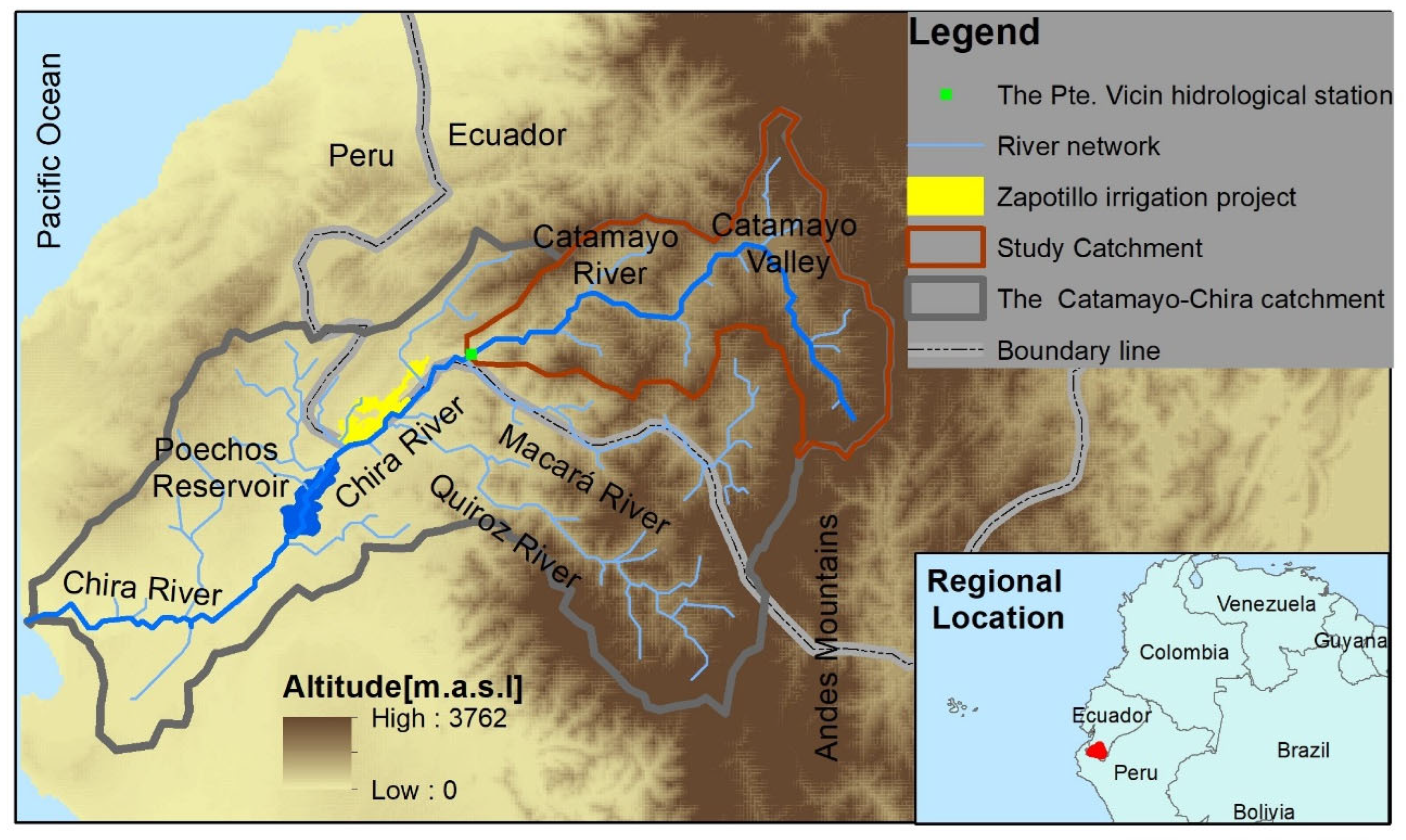
2.1. Study Catchment

The research area encompasses the Catamayo catchment, with its outlet defined by the Pte. (a Spanish abbreviation for bridge) Vicin hydrological station (catchment area: 4174.5 km²). The altitude of this area ranges from 257 to 3762 m.a.s.l in the Andean Cordillera. This catchment includes the middle and upper sections of the cross-border Catamayo-Chira catchment; a Pacific–Andean system in southern Ecuador and northern Peru (Figure 1). Originating from humid, high-altitude regions within the Andean Cordillera, the Catamayo catchment descends through semi-humid and semi-arid regions in its low part, though isolated aridity areas can be found in the eastern part of the catchment, such as the Catamayo Valley (Figure 1). These latter zones, characterised by a drier climate, are the most vulnerable to drought. This unique occurrence is attributed to the catchment’s distinctive topography, which is marked by various small ridges and intersecting valleys in contrast to the two distinct mountain chains observed in the Ecuadorian and Peruvian Andes.

In the lower reaches of the cross-border Catamayo-Chira catchment (0–80 m.a.s.l), there is a brief wet season from January to April, with annual precipitation varying between 10 and 80 mm. Moving from these lower areas to the upper segments, the duration of the wet season extends, and precipitation increases, particularly in the middle and upper areas (the study zone). Within the Catamayo catchment, the wet season spans from October to May, with March being the peak month for precipitation, as identified by Pineda et al. (2013) [21]. The El Niño–Southern Oscillation (ENSO) phenomenon, particularly its negative phase, significantly influences precipitation patterns. Above 800 m.a.s.l, precipitation is primarily influenced during strong negative ENSO years, recording average depths of 984 mm in “normal” years and 1646 mm during strongly negative ENSO years [22].

The catchment’s geology is predominantly characterised by the presence of intrusive rocks from the Neocene and Paleocene epochs, including volcanic and granitoid formations found in the Andes (for example, the Formación Volcánico Porculla and Volcánico Llama) and by Upper Cretaceous sedimentary and volcanic formations in the lowland regions [23]. Owing to the study catchment’s location in the upper region, there are no productive aquifers within the catchment, although there are specific areas where aquifers of low productivity can be found. The primary groundwater reserves have been identified downstream of the catchment outlet, where significant exploitation occurs [24,25].

Within this catchment, two major irrigation initiatives stand out: the Ecuadorian Zapotillo irrigation project and the Peruvian Poechos reservoir, both situated downstream of the study area (refer to Figure 1). These projects are sustained by the surface water resources of the catchment. Together, they facilitate the irrigation of approximately 11,500 hectares.

2.2. Data Description

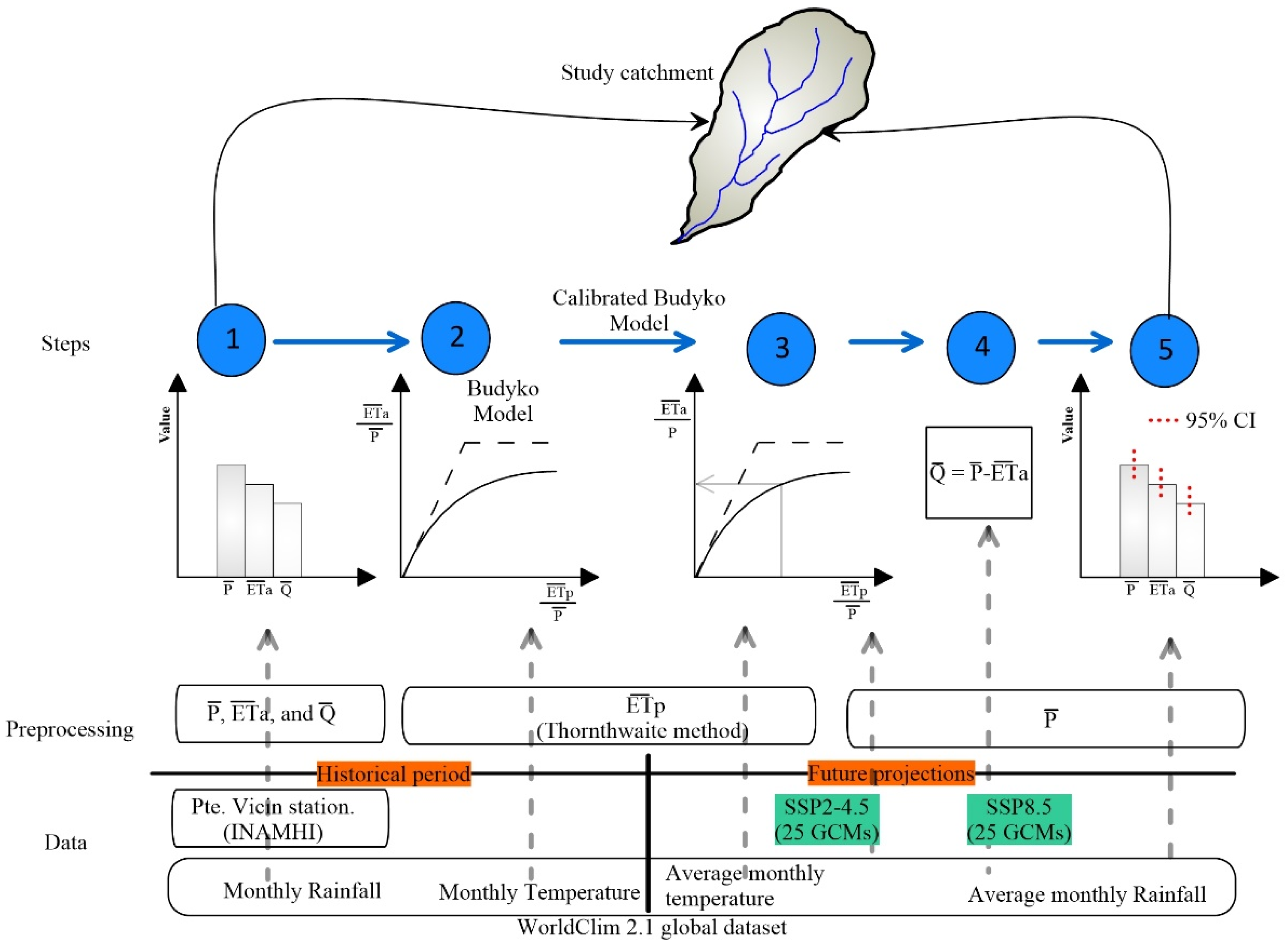
To predict the impact of climate change on the average annual water balance of a catchment, it is essential to utilise both historical data and future climate projections. Due to the limited data characteristics and the peculiar topography of the catchment, we sourced historical monthly precipitation and temperature from the WorldClim 2.1 global dataset [26] for the historical period 1990–2011, as well as their average monthly estimates for the near (2021–2040), mid (2041–2060), and far (2061–2080) futures. We also included streamflow data from the Pte. Vicin hydrological station, taken from the database of Ecuador’s Meteorological Service—Instituto Nacional de Meteorología e Hidrología del Ecuador (INAMHI)-, covering the same historical period (1990–2011) as detailed in

Table 1. Description of the historical and future data.

Variable	Temporal Resolution	Time Period	Spatial Resolution	Source/Description
Streamflow [m3/s]	Monthly	1990–2011	-	Records of the Pte. Vicin station. (INAMHI)
Maximum, minimum, and average * temperature [°C]			~5 km	WorldClim 2.1 https://www.worldclim.org/data/index.html (accessed on 5 March 2024)
Precipitation ** [mm]
Precipitation [mm]	Average monthly	2021–2040 2041–2060 2061–2080
Maximum, minimum, and average * temperature [°C]

* The average temperature for the historical period and future projections was obtained as the mean of the maximum and minimum temperature WorldClim data. ** The period 1990–2011 was used for the mean annual water balance analysis, while the period 1960–2020 was used for analysing precipitation deficits.

. For the analysis of precipitation deficits, we utilised the WorldClim 2.1 monthly precipitation data for the period 1961–2020, aggregated to annual values. The use of the WorldClim 2.1 global dataset, which has been increasingly used in this region [27,28], allowed for a comparison between the WorldClim-based estimates and those derived from limited local records reported in other studies.

2.3. Methodology

2.3.1. General Description of the Water Balance Framework

Figure 2 provides an illustration of the water balance framework employed in this study, which comprises five fundamental steps. Initially, the mean annual catchment values for precipitation ($\overline{P}$), actual evapotranspiration (${\overline{ET}}_a$), and runoff ($\overline{Q}$) are estimated from historical monthly records (Step 1). These variables are then utilised to calibrate a Budyko model for the catchment (Step 2). Subsequently, this calibrated model is applied to future projections to calculate future actual evapotranspiration based on the future aridity index (${\overline{ET}}_p$/$\overline{P}$), which is determined using the future projections of average monthly precipitation and temperature from the WorldClim 2.1 global dataset (Step 3). The future runoff is then computed as the difference between the mean annual precipitation and actual evapotranspiration (Step 4). These steps (Steps 3 and 4) are executed for two climate change scenarios: SSP2-4.5 (a ‘Middle of the road’ scenario) and SSP8.5 (a ‘Fossil fuel-driven development’ scenario), considering 23 General Circulation Models (GCMs). This approach enables the quantification of the 95% confidence interval (Step 5) for future projections. A detailed description of these steps is provided below.

2.3.2. Calculation of the Mean Annual Water Balance Variables for the Historical Period

In Step 1 of the framework, the value of $\overline{P}$ in Equation (1) was calculated as the mean of the 5 km- WorldClim average annual precipitation data across the catchment. This was achieved by aggregating the 5 km monthly WorldClim data into annual values and then computing the average. Similarly, the average annual runoff $\overline{Q}$ was determined from the mean of the yearly streamflow measurements at the Pte. Vicin hydrological station. This figure was then converted into millimetres per year (mm/year) by dividing by the catchment’s area, ensuring a consistent measurement scale. Finally, the catchment’s mean annual actual evapotranspiration ${\overline{ET}}_a$ was calculated as the difference between $\overline{P}$ and $\overline{Q}$.

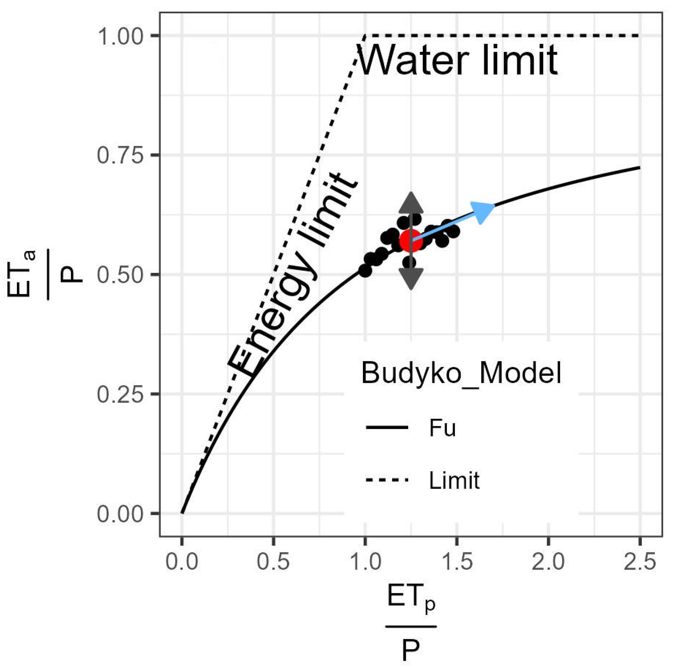
2.3.3. Budyko Framework

The mean annual water balance equation, expressed by Equation (1), is applicable under conditions when equilibrium exists among the water balance variables $\overline{P}$, ${\overline{ET}}_a$, $\overline{Q}$, and the mean annual change of water storage ($∆\overline{S}$) may be considered insignificant for the long-term. To attain this state of equilibrium, there should be also an absence of external disruptions influencing the water balance, such as the extraction of groundwater or the transfer of water to or from other catchments.

It posits that the partitioning of $\overline{P}$ and ${\overline{ET}}_a$ is a function of the relative supply of water, represented by $\overline{P}$, and the atmospheric demand for water, represented by the catchment-wide estimate of the mean annual potential evapotranspiration ${\overline{ET}}_p$, which is influenced by the available energy. Consequently, this framework establishes the “Budyko space”, which accounts for the water and energy constraints of the catchment as depicted in Figure 3, stipulating that evapotranspiration cannot exceed the atmospheric demand and the catchment cannot evapotranspirate more water than it receives from its water source ($\overline{P}$).

It merits mention that the Budyko framework is an empirical method that devises a curve within the Budyko space to delineate the average behaviour of several catchments under study. Subsequently, the framework has been expanded to individual catchments to describe the relationship between the actual evapotranspiration ratio (${\overline{ET}}_a$/$\overline{P}$) and the aridity index (${\overline{ET}}_p$/$\overline{P}$) through the use of parametric equations. Among the most prevalent is the Fu equation [18,29], which allows a parameter $w$ to be calibrated that reflects catchment characteristics:

$${\displaystyle \frac{{\overline{ET}}_a}{\overline{P}}}=1+{\displaystyle \frac{{\overline{ET}}_p}{\overline{P}}}-{\left[1+{\left({\displaystyle \frac{{\overline{ET}}_p}{\overline{P}}}\right)}^w\right]}^{{\displaystyle \frac{1}{w}}}$$

(2)

This empirical parameter allows the specific placement of the catchment within the Budyko space. Should a Budyko model be utilised on an annual basis for a catchment with stable characteristics, there would be a dispersion around the curve of the annual values for a particular year owing to the intra-annual fluctuations of the climate cycle. The Budyko curve and its associated parameter illustrate the average behaviour of the catchment (Figure 3). The impact of climate change on the catchment could be depicted by a shift along this curve (Figure 3, light blue arrow) or by a deviation from the initial curve (Figure 3, dark grey arrows). This topic has been the subject of discussion in various studies [8,15], and one of the aims of this work is to contribute to this debate by presenting the results from the study catchment.

2.3.4. Calibration of the Budyko Model for the Study Catchment

The future projections of the mean annual actual evapotranspiration ${\overline{ET}}_a$ were calculated using the Budyko framework, as it facilitates the estimation of ${\overline{ET}}_a$ as a function of the aridity index, ${\overline{ET}}_p$/$\overline{P}$. In turn, ${\overline{ET}}_p$ can be calculated based on future temperature projections, the primary future climate variable considered in this study (Table 1).

The calibration of the parameter $w$ in Equation (2) aims to incorporate the combined effects of climatic conditions (e.g., precipitation seasonality) and catchment characteristics (e.g., vegetation cover, soil properties, and catchment topography) on the water balance [5,30,31]. Model calibration was based on historical data for the period 1990–2011 (Figure 2, Step 2). Firstly, the historical temperature data, i.e., the 5 km WorldClim monthly values (Table 1), were used to calculate average monthly figures, allowing the calculation of the catchment’s mean annual potential evapotranspiration ${\overline{ET}}_p$. This was achieved through the Thornthwaite method, first determining the 5 km average monthly potential evapotranspiration (${ET}_{p_j}$), aggregating these figures then into annual values, and finally averaging these to obtain the catchment-wide estimate (i.e., ${\overline{ET}}_p$). Thornthwaite’s formula has been successfully applied for large-scale potential evapotranspiration and aridity assessments in different climatic zones, being favoured for its lower data requirements compared to other methods [32]. It has been demonstrated that the use of more complex models, such as the well-known Penman–Monteith method, does not yield significant improvements in studies based on the Budyko approach [15]. In a study of climate change using seven potential evaporation formulations covering a range of complexity, ref. [33] concluded that due to the codependence of climatic variables with respect to temperature the formulations all showed similar future trends.

Grids of ${ET}_{p_j}$ were, thus, calculated according to the following formula [34]:

$${ET}_{p_j}=16{\left({\displaystyle \frac{10T_j}{I}}\right)}^a·f_{c_j}$$

(3)

where

• ${ET}_{p_j}$: average potential evapotranspiration for the month $j$ [mm/month];
• $T_j$: average temperature for the month $j$ [°C];
• $I$: the annual heat index defined as the sum of 12 monthly value of $i$ where $i={\left(T_j/5\right)}^{1.514}$
• a: $\left(6.75\times {10}^{-7}\right)·I^3-\left(7.71\times {10}^{-5}\right)·I^2+\left(1.79\times {10}^{-2}\right)·I+0.492$
• $f_{c_j}$: correction factor for the month $j$ based on number of daylight hours per day compared to 12 and number of days in a month compared to 30. Therefore, this value depends also on the latitude. Some values of this factor are described in

  Table 2. Values of the correction factor $f_c$ used in the Thornthwaite equation for each month and latitudes from 10° N to 10° S.

  Lat.	Jan.	Feb.	Mar.	Apr.	May	Jun.	Jul.	Aug.	Sep.	Oct.	Nov.	Dec.
  10° N	1.00	0.91	1.03	1.03	1.08	1.05	1.08	1.07	1.02	1.02	0.98	0.99
  5° N	1.02	0.93	1.03	1.02	1.06	1.03	1.06	1.05	1.01	1.03	0.99	1.02
  Ecuador	1.04	0.94	1.04	1.01	1.04	1.01	1.04	1.04	1.01	1.04	1.01	1.04
  5° S	1.06	0.95	1.04	1.00	1.02	0.99	1.02	1.03	1.00	1.05	1.03	1.06
  10° S	1.08	0.97	1.05	0.99	1.01	0.96	1.00	1.01	1.00	1.06	1.05	1.10

  .

Subsequently, the catchment’s mean annual potential evapotranspiration estimate ${\overline{ET}}_p$ was used to calculate the aridity index, ${\overline{ET}}_p$/$\overline{P}$. Then, the catchment mean annual actual evapotranspiration ${\overline{ET}}_a$ was calculated as the difference between $\overline{P}$ and $\overline{Q}$ (Equation (1)) to subsequently compute the actual evapotranspiration ratio, ${\overline{ET}}_a$/$\overline{P}$. These indexes were employed as input parameters in Fu’s equation to adjust the parameter $w$ (Equation (2)) using an optimisation function based on the Newton’s method. To determine this value, Equation (2) was rearranged to form an expression equal to zero, and ω was iteratively computed as the value that satisfies this condition, i.e., closure of the water balance with minimal error. The fitted $w$ parameter was finally used in Equation (2) to project future variables of the mean annual water balance, as detailed in the subsequent subsection.

2.3.5. Calculation of the Mean Annual Water Balance Variables for the Future Scenarios

The future projections of $\overline{P}$ were estimated by first aggregating the future 5 km-WorldClim average monthly precipitation (Table 1) into annual values, and finally averaging these to obtain the catchment-wide estimate. Subsequently, this future value of $\overline{P}$, alongside the future estimate of ${\overline{ET}}_p$ and catchment Budyko model, was employed to project the future mean annual actual evapotranspiration ${\overline{ET}}_a$ based on Equation (2) and the fitted parameter $w$ (Step 3, illustrated in Figure 2). The future value of mean annual potential evapotranspiration ${\overline{ET}}_p$ was first calculated by determining the grids of (5 km × 5 km) average monthly potential evapotranspiration ${ET}_{p_j}$, using the 5 km WorldClim average monthly future temperature (Table 1) and Thornthwaite equation (Equation (3)). These ${ET}_{p_j}$ grid values were then aggregated into annual totals and averaged to derive the catchment-wide estimate. Finally, the mean annual runoff $\overline{Q}$ was projected by calculating the difference between the future values of $\overline{P}$ and ${\overline{ET}}_a$ (Step 4, illustrated in Figure 2).

2.3.6. Climate Change Impact Estimate on Water Availability (Significance and 95th Percentile Band)

The calculation of the mean annual water balance variables is conducted for each General Circulation Model, GCM, output under two climate change scenarios: SSPP2-4.5 (“Middle of the road scenario”) and SSP8.5 (“Fossil fuel-driven development scenario”) (Step 5, illustrated in Figure 2). The GCMs included in this study are those featured in the WorldClim 2.1 global dataset (https://rdrr.io/github/rspatial/geodata/man/cmip6.html, accessed on 5 March 2024). These are downscaled future climate projections where the downscaling and calibration (bias correction) was done within WorldClim v2.1 (for details of the downscaling procedure, go to https://www.worldclim.org/data/downscaling.html, accessed on 5 March 2024). Three models were omitted from the analysis (BCC-CSM2-MR, GFDL-ESM4, and MRI-ESM2-0) due to inconsistencies in the temperature and/or precipitation data they provided for the study catchment.

The mean of the GCM future projections of water balance variables were used within the water balance framework to assess impacts on future water availability. Projections for three 20-year future periods (2021–2040, 2041–2060, and 2061–2080) were used. To capture the level of confidence in the estimate of the mean, a 95% predictive interval, which is a common measure in climate change studies [17], was calculated as follows:

$$95\% \mathrm{Confidence} \mathrm{interval}=\overline{x}\pm t_{0.025}\left({\displaystyle \frac{s}{\sqrt{n}}}\right)$$

(4)

where

• $\overline{x}$: sample mean of the future projections;
• $t_{0.025}$: t-score with area in the right and left tails equal to 0.025;
• $s$: sample standard deviation of the future projections;
• $n$: sample size of the future projections.

The statistical significance of the climate change projections was assessed by comparing the 95th percentile band, representing the future variability of water balance variables, with estimates from the historical period. If the historical values fall within this 95th percentile band, it is assumed that there is no significant change at the 5% level of significance. It is important to emphasise that this ensemble approach, employing multiple GCMs to capture a range of outcomes, is frequently advocated in climate change research. This strategy aims to accommodate model variability and furnish more reliable projections [35].

2.3.7. Precipitation Deficit Analysis and Future Deficit Projections Under Climate Change

While a mean annual water balance provides the cornerstone of any water availability assessment for a catchment, it does not provide any information on year-to-year variability. The hydrological regimes of South American catchments are known to be highly variable due to ENSO and other factors influencing natural climatic variability. In particular, regional precipitation regimes have been shown to exhibit long-term persistence (LTP), which is characterised by the Hurst coefficient H (0.5 < H < 1); as H increases, LTP increases, resulting in longer runs of years above or below the mean. In an analysis of annual average precipitation for 8 global regions based on GPCC gridded (0.5 × 0.5 degrees) data for the period 1900–2013 [36], O’Connell et al. (2022) [37] found Hurst coefficients of 0.73 and 0.78 for annual precipitation averaged over regions covering the Amazon and Southern South America, respectively, indicating strong LTP (H > 0.7). They also found that LTP increased with the spatial scale of averaging, with pixel scale (0.5 × 0.5 degrees) of H of 0.63 and 0.69, respectively. Strong LTP for the regions analysed was shown to be related to long-term modes of variability in the climate, specifically the Southern Oscillation Index (SOI), the Interdecadal Pacific Oscillation (IPO) and the Pacific Decadal Oscillation (PDO) (El Nino is a relatively short-term oscillation). This variability presents a major challenge in managing multi-year water resources deficits.

To provide some measures of variability for the Catamayo catchment, an analysis of precipitation deficits below the mean has been undertaken using the WorldClim annual precipitation data for the period 1961–2020; the runoff record is not sufficiently long to support such an analysis. This has been based on deficits below the means of 20-year periods because the GCM projections of mean precipitation used here are based on 20-year periods, and the results of the deficits analysis can therefore be applied to these 20-year means. A 20-year time window has also been used by Santos et al. (2024) [38] in analysing annual and monthly precipitation anomalies over Ecuador using WorldClim CMIP6 GCM ensemble projections.

A volume deficit is defined as the cumulative sum of deviations below the mean of each 20-year period ($X_j$ $-$ $\overline{X}$), $X_j$ < $\overline{X}$, for a deficit period of duration $D_i$ = 1, 2, 3, … years, where $\overline{X}$ is the historical (60-year) mean. There will be several such deficits for each duration $D_i$ in a time series of length $n$, so each volume deficit is designated as $V_{i,k.}$. These volume deficits are then standardised by the mean and converted to a percentage to give a standardised percentage volume:

$${SV}_{i,k}=\left({\displaystyle \frac{V_{i,k}}{\overline{X}}}\right)100$$

(5)

The average percentage deficit volume for a duration $D_i$ is defined as

$${\overline{SV}}_i={\displaystyle \frac{\sum _1^m{SV}_{i,k}}{m_i}}$$

(6)

and the average percentage deficit intensity as

$${\overline{SI}}_i={\sum }_1^m{\displaystyle \frac{\frac{{SV}_i}{D_i}}{m_i}}$$

(7)

where $m_i$ is the number of deficits of duration $D_i$.

If $f_i$ denotes the relative frequency of a deficit of duration $D_i$, then the expected duration of a deficit duration, percentage volume and percentage intensity of a deficit can be defined as follows:

$$E\left(D\right)={\sum }_1^P{f}_i{D}_i$$

(8)

$$E\left(SV\right)={\sum }_1^P{f}_i{\overline{SV}}_i$$

(9)

$$E\left(SI\right)={\sum }_1^P{f}_i{\overline{SI}}_i$$

(10)

where $p$ denotes the number of relative frequencies covering the observed number of deficits. These expressions provide measures of the average properties of deficits in a 20-year period, as the deficits have been defined with respect to 20-year means.

3. Results and Analysis

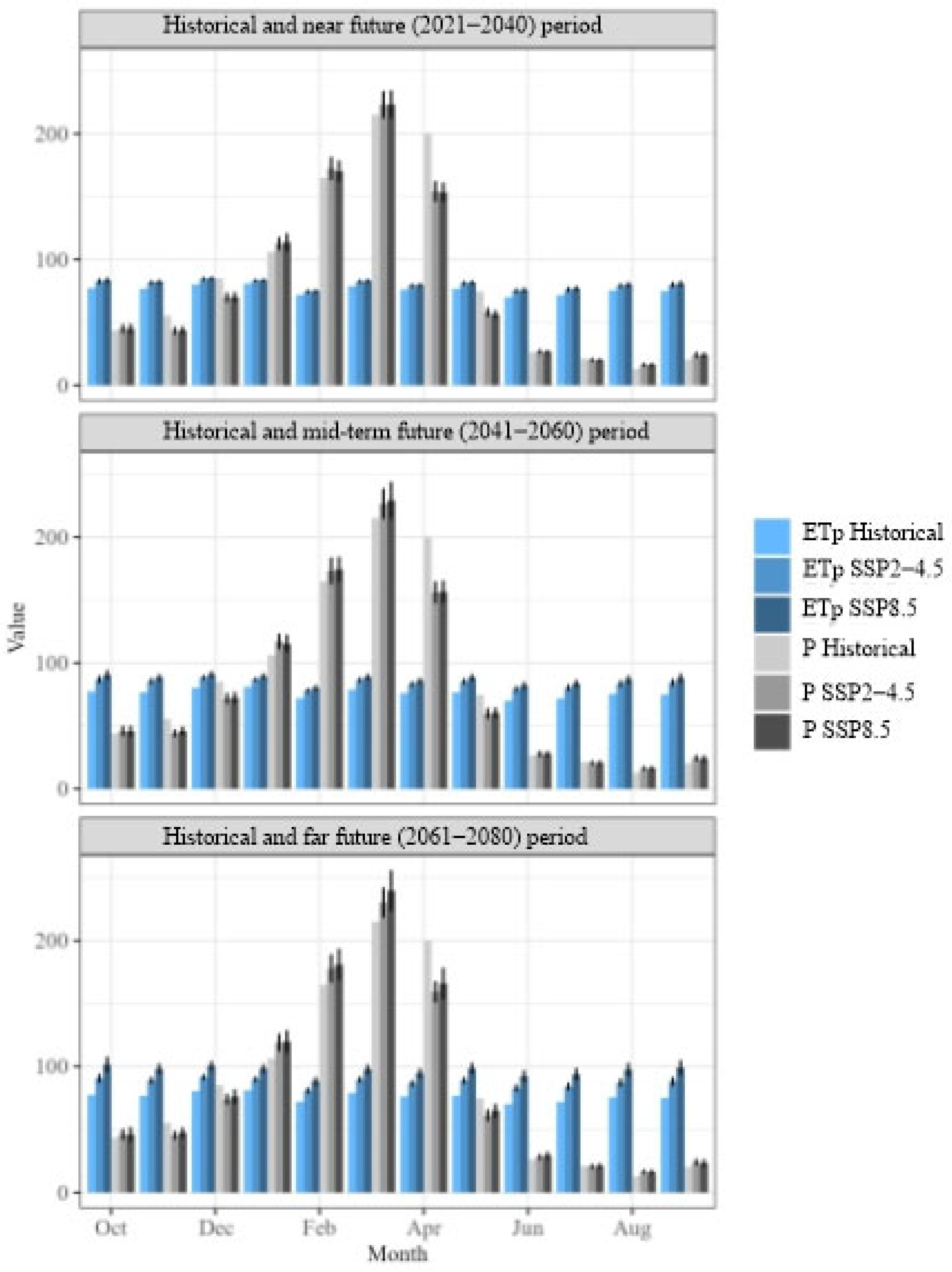
3.1. Historical 5 Km Grid Values of Climate Variables and Future Projections

Figure 4 displays the mean annual historical climate data (including precipitation, temperature, and potential evapotranspiration) over a 5 km grid, along with future projections. These estimates are based on the averages of 23 General Circulation Model (GCM) outputs under the SSP2-4.5 and SSP8.5 scenarios for the far future (2061–2080). Meanwhile,

Table 3. Climate change impact on the mean annual precipitation, temperature, and potential evapotranspiration within the Catamayo Catchment, as well as the associated confidence bands for the far future (2061–2080). Future values are presented in units and as percentages relative to the historical mean. Values highlighted in italics signify the historical mean falls inside the confidence band.

Variable/Scenario	Historical	SPP2-4.5	SSP8.5
$\overline{P}$ [mm]	1023	1005 ± 53 −1.8 ± 5.2%	1040 ± 69 +1.6 ± 6.7%
$\overline{T}$ [°C]	19	21.14 ± 0.27 +11.3 ± 0.01%	22.3 ± 0.38 17.2 ± 0.02%
${\overline{ET}}_p$ [mm]	892	1075 ± 25 +20.5 ± 0.03%	1194 ± 45 +33.8 ± 0.05%

lists the catchment values and their associated 95% confidence interval, calculated using Equation (4).

Before comparing and discussing the results of the climate change impacts on the catchment-wide estimates, it is important to analyse the spatial distribution of the mean annual values over the catchment and their future projections. As one can see in Figure 4, the temperature demonstrates a strong correlation with altitude, displaying higher values in lowland regions and lower values in upland areas, as expected. This pattern is mirrored in the potential evapotranspiration, which, like temperature, is influenced by altitude, owing to the Thornthwaite method being based solely on temperature. The historical precipitation data on the other hand reveals the highest precipitation depths on the upper eastern ridge of the catchment (Andean mountains, Figure 1). This phenomenon results from the prevailing easterly winds that transport moisture from the Amazon catchment to the eastern mountain ridge. The pronounced barrier effect of this mountain range significantly obstructs moisture transport within the watershed. Additionally, a specific area in the upper eastern part of the catchment displays lower precipitation volumes than its surroundings (Catamayo valley, referenced in Figure 1), due to its orographic position encircled by mountain barriers that restrict moisture flow from all directions. The precipitation map also indicates values between 600 and 650 mm and potential evapotranspiration values above 1200 mm at the catchment outlet, a semi-arid zone, with these figures being consistent with records reported by Ochoa et al. (2016) [39], where precipitation are generated by westerly winds that bring humid air from the Pacific Ocean. Regarding future projections for the far future, 2061–2080, the results indicate a significant increase in both the average annual temperature and potential evapotranspiration in these zones; note how the potential evapotranspiration increases in these zones considerably, whereas the precipitation is very similar. These maps indicate that these future projections suggest an increase in aridity in the semi-arid (catchment outlet) and arid (Catamayo valley) zones of the Catamayo Catchment.

The historical catchment-wide estimate for potential evapotranspiration is 892 mm, while the historical mean annual temperature is approximately 19 °C. This last value is consistent with that derived from the observed temperature gradient with altitude within the catchment, as reported by Ochoa et al. (2016) [39]. The catchment’s average annual precipitation is 1023 mm, a figure similar to the ~1040 mm estimate based on the records reported by the same authors and using an ordinary Kriging technique. These findings suggest that the historical catchment-wide estimates based on the 5 km gridded WorldClim data are consistent with those reported by other studies.

By comparing historical catchment-wide averages, future projections for the far future indicate temperature rises of 11.3 ± 0.1 °C and 17.2 ± 0.3 °C, along with increases in average potential evapotranspiration of 20.5 ± 0.03% and 33.8 ± 0.05% under the SSP2-4.5 and SSP8.5 scenarios, respectively (Table 3). Average precipitation within the catchment is projected to show slight fluctuations compared to the historical figure of 1023 mm, with these changes being almost negligible on annual maps. Specifically, there is a projected decrease of 1.8 ± 5.2% under SSP2-4.5 and a modest increase of 1.6 ± 6.7% under SSP8.5.

A related climate change study, extending up to 2050 for the contributing catchment of the Poechos Reservoir, also reported a temperature increase, whereas the results for precipitation were ambiguous, showing both a decrease and increase in different months of the year [40]. Note that, in this work, the historical precipitation mean (1023 mm) falls inside of the 95% confidence interval of the future projections under the two scenarios (Table 3), which does not allow one to conclude that this variable is increasing or decreasing with respect to the historical period. However, for mean annual temperature and potential evapotranspiration, the scenarios indicate clear increases in these variables (Table 3). As highlighted by Almazroui et al. (2021) [35], quantifying the confidence in climate change estimates is crucial for producing more reliable projections.

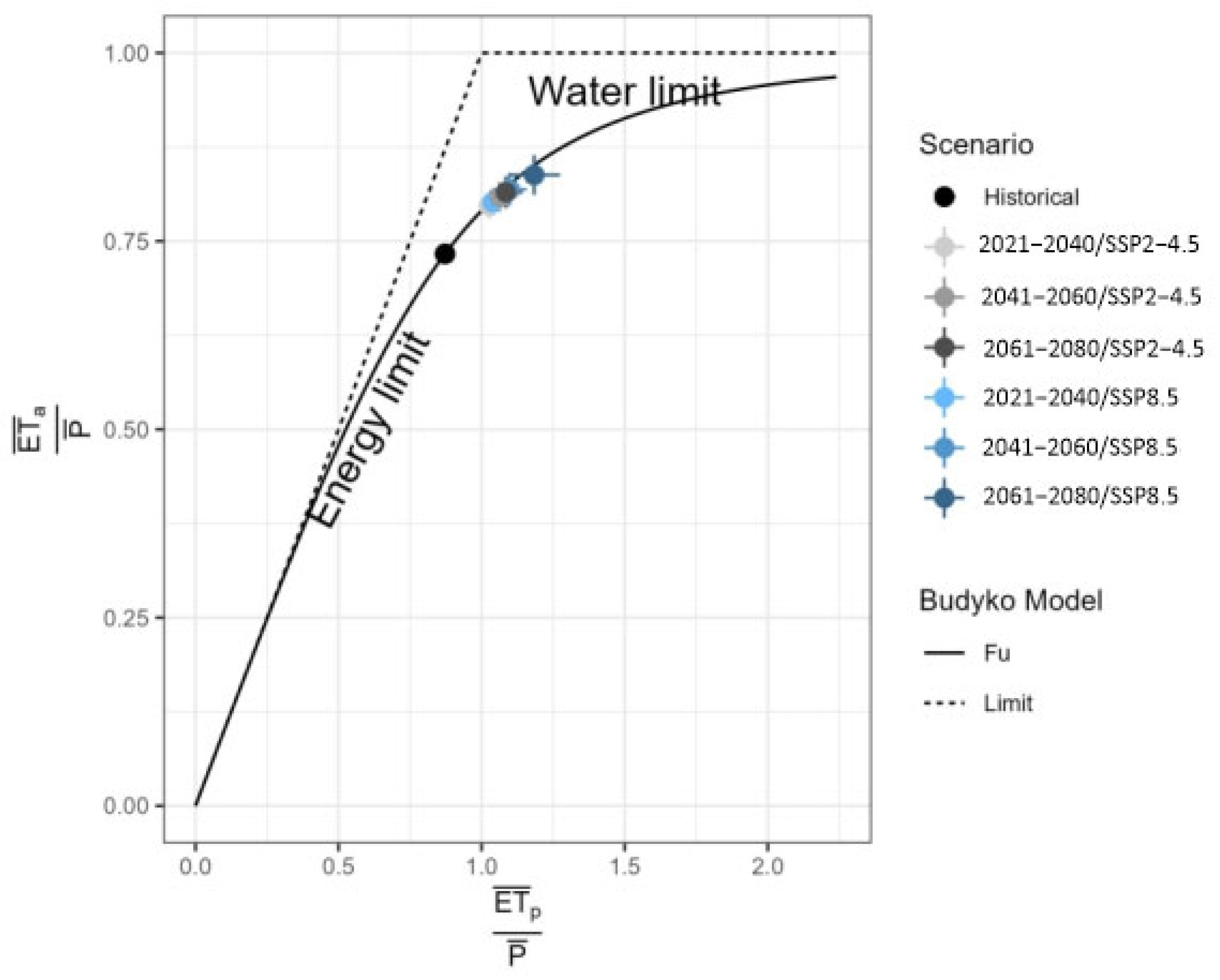
3.2. Budyko Model and Future Projections

Figure 5 shows the relationship between the evapotranspiration rate and aridity indices. The dotted lines represent the energy limit (no more energy, represented by potential evapotranspiration, can be consumed than is available) and the water limit (no more water, represented by actual evapotranspiration, can be consumed than is available). As shown in this figure, the average relationship between these two indexes, i.e., between ${\overline{ET}}_a/\overline{P}$ and ${\overline{ET}}_p/\overline{P}$, respectively, based on historical records in the study catchment (black point), has been calibrated to match Fu’s curve with $w$ = 3.65. This value can be considered high which means that a significant portion of the precipitation is used for evapotranspiration, with less becoming runoff; the higher $w$, the closer the curve comes to the energy and water limit lines (Figure 3 and Figure 5). In other words, this parameter is related to the ability of a watershed to retain water for evapotranspiration [41]. High values in the study zone indicate well-developed retention capacities and efficient actual evapotranspiration.

The vertical and horizontal lines at these points indicate the 95% confidence intervals, representing the variability in the evapotranspiration rate and aridity indices derived from the selected set of 23 GCM outcomes. It is significant to observe that the confidence associated with these indices is generally high, indicating consistency across GCM outcomes. However, under scenarios featuring a marked increase in temperature, particularly in the 2061–2080/SSP8.5 scenario, this minimal variability is seen to slightly rise. In such a scenario, it is noteworthy that the variability associated with the aridity index is significantly higher than that related to the evapotranspiration rate. This observation supports the notion that the variability in the estimates of precipitation and potential evapotranspiration does not directly affect actual evapotranspiration as predicted by Fu’s equation. Particularly, the variability in the estimation of actual evapotranspiration (${\overline{ET}}_a$) based on Equation (2) is, as will be seen later on (Section 3.3), substantially lower than the considerable variability found in $\overline{P}$.

The influence of climate change within the Budyko framework is, on the other hand, signalled by a displacement along this curve. It is noteworthy, however, that as the catchment’s average response begins to diverge slightly from the initial curve under scenarios with a pronounced increase in temperature, this divergence becomes particularly evident in the 2061–2080/SSP8.5 scenario. These findings concur with those of Jaramillo et al. (2022) [15], who assert that the deviation in average catchment behaviour from the Budyko curve can be attributed not only to changes in hydrological properties, due to anthropogenic interventions such as river management, irrigation, and land cover alterations, but also to climate change. This observation leads to the proposal of the “catchment trajectory conjecture” by Reaver et al. (2022) [42], which postulates that catchments would adhere to a typical Budyko curve trajectory (Figure 3, light blue arrow) if it were not for the alterations in hydrological properties that are independent of changes in the average aridity index.

Figure 5 also reveals that the historical long-term average aridity index is 0.87, signifying that the catchment’s average climate can be classified as sub-humid, according to Ponce et al. (2000) [43]. It is worth noting that this classification pertains to an “average” climate assessment of the catchment. However, readers should bear in mind, as highlighted in the previous section, that the catchment outlet includes a semi-arid zone, and there is a small arid area in the upper eastern part of the catchment (the Catamayo Valley, Figure 1), which, according to the findings of this work, does not significantly impact the average estimates. However, as mentioned in the prior section (Section 3.1), the results suggest that the aridity in these zones will increase.

Aligned with this observation, it is significant to note that the climate change projections suggest an increase in the historical long-term average aridity index greater than one. This indicates that the average annual potential evapotranspiration, under the future scenarios, surpasses the average annual precipitation. Such a shift results from the null change in precipitation patterns (statistically speaking) and the increase in evapotranspiration rates, as discussed in the preceding section. It is particularly intriguing to explore how these behaviours manifest on a seasonal basis. The dynamics of these changes, along with their associated confidence bands, are detailed in Figure 6 and explained as follows.

Regarding the future estimates of potential evapotranspiration, Figure 6 illustrates a similar absolute increase across all 12 months, with small and consistent variability throughout the period. The results also show this variable remains relatively stable throughout the year, as does the temperature (specific values are not shown here).

Regarding the future precipitation estimates, the results demonstrate varied patterns during the 12 months, with an increase from January to March, a decrease in the subsequent two months (April and May), with no significative changes until October, and a decrease from November to December.

The variability linked to these estimates is minimal but rises in tandem with precipitation depths, reaching its peak in March, the wettest month. It is crucial to acknowledge that historical data for the rainy season (October–May) are significantly influenced by Negative ENSO events. There is evidence that ENSO events will intensify in the future Hu et al. (2021) [44], which may increase precipitation depths from December to March, as demonstrated in this study. While the CMIP6, which forms the basis for these future projections, has shown enhanced accuracy over its Phase 5 predecessor (CMIP5) in simulating ENSO characteristics, this finding should be approached with caution. Hou and Tang (2022) [45] concluded that CMIP6′s performance in capturing ENSO can still be considered modest. The analysis of the seasonality shown in Figure 6 indicates that the future variations in precipitation depths, compared to historical values, during the rainy season will result in a future mean annual value that is similar to the historical average. This future seasonality variation is the reason why the historical precipitation values fall within the confidence band of the future estimates, as shown in Table 3.

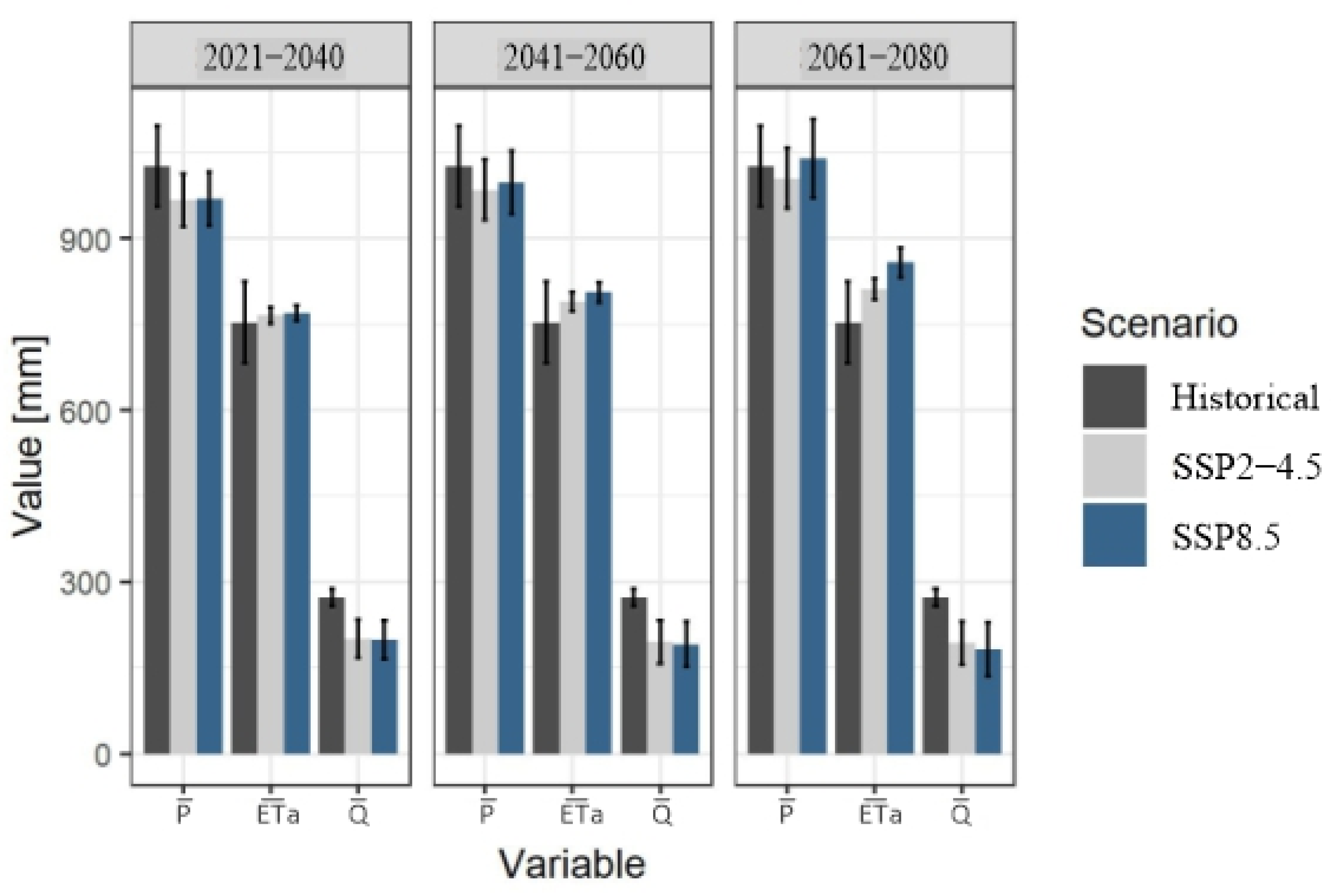
3.3. Climate Change Impact on the Mean Annual Water Balance in the Study Catchment

Figure 7 depicts the historical mean annual water balance variables, and future estimates with their associated 95th percentile band for the study catchment; their values are presented in

Table 4. Climate change impact on the mean annual water balance variables within the Catamayo Catchment, as well as the associated confidence bands for the near, mid, and far future. Future values are presented in units and as percentages relative to the historical mean. Values highlighted in italics signify the historical mean falls inside the confidence band.

Variable	Scenario	1990–2011	2021–2040	2041–2060	2061–2080
$\overline{P}$ [mm]	Historical	1023
	SPP2-4.5		967 ± 47 −5.5 ± 4.6%	985 ± 52 −3.7 ± 5.1%	1005 ± 53 −1.8 ± 5.2%
	SSP8.5		969 ± 47 −5.3 ± 4.6%	997 ± 55 −2.5 ± 5.4%	1040 ± 69 +1.6 ± 6.7%
${\overline{ET}}_a$ [mm]	Historical	750
	SPP2-4.5		766 ± 15 2.1 ± 1.9%	790 ± 17 5.3 ± 2.2%	812 ± 18 8.2 ± 2.4%
	SSP8.5		769 ± 14 2.54 ± 1.9%	806 ± 18 7.4 ± 2.4%	858 ± 26 14.3 ± 3.5%
$\overline{Q}$ [mm]	Historical	273
	SPP2-4.5		201 ± 34 −26.3 ± 12.3%	195 ± 37 −28.5 ± 13.7%	193 ± 37 −29.2 ± 13.7%
	SSP8.5		200 ± 34 −26.8 ± 12.3%	191 ± 39 −29.9 ± 14.4%	182 ± 46 −33.3 ± 17.0%

. The results show that, for the historical period, the mean annual values of the study catchment for actual evapotranspiration and runoff are 750 and 273 mm, respectively.

With regard to the variability of future estimates, it is notable how it increases with more distant time slices for all variables, these results are in line with those reported by Shen et al. (2018) [46]. The confidence band remains broadly consistent for each variable across different scenarios within the same time window, except in the far future (2061–2080), where the 95th percentile band of variables increases under the worst-case scenario (SSP8.5). The results also reveal that the estimation of $\overline{P}$ exhibits the highest variability, runoff ($\overline{Q}$) displays an intermediate level of confidence, and actual evapotranspiration (${\overline{ET}}_a$) has the lowest. Interestingly, the variability in the estimation of ${\overline{ET}}_a$, as calculated based on Equation (2), is substantially lower than that of $\overline{P}$, one of its inputs. These findings suggest that when estimating future values of mean annual actual evapotranspiration ${\overline{ET}}_a$ using Fu’s equation, the lower confidence associated with the future mean annual precipitation $\overline{P}$ is not proportionally reflected in ${\overline{ET}}_a$. This ${\overline{ET}}_a$ low variability arises from the insensitivity of ${\overline{ET}}_p$, associated to the Thornthwaite method, and the Fu’s equation, which acts as a “filter”, increasing the confidence in ${\overline{ET}}_a$. Note that the slope of the Budyko curve, defined by Fu’s equation, starts to decrease for aridity indexes (${\overline{ET}}_p/\overline{P}$) greater than 1 (Figure 5), which also reduces the variability of the actual evapotranspiration ratio (${\overline{ET}}_a/\overline{P}$) and, therefore, of ${\overline{ET}}_a$.

Considering the mean of future projections, the results demonstrate that climate change leads to a reduction in mean annual precipitation across all scenarios and time windows, with the sole exception being the far future for the SSP8.5 scenario (2061–2080/SSP8.5 scenario), which exhibits a slight increase of 1.6 ± 6.7% (Table 4). It is noteworthy, as analysed in Section 3.1, that the historical mean precipitation also falls within the 95th percentile band of future estimates for the mid future for the two scenarios (Table 4), whereas for the near future the upper band almost reaches the historical mean. This overlap prevents a definitive conclusion regarding the trend of this variable compared to the historical period. However, this situation does not apply to the mean annual actual evapotranspiration and runoff (Table 4), where it can be concluded that there will be a significant increase and decrease in these variables, respectively, across all scenarios and time windows. For the mean actual evapotranspiration, the results suggest that, for the SSPP2-4.5 scenario, there will be an increase of 2.1 ± 1.9%, 5.3 ± 2.2%, and 8.2 ± 2.4% for the near, mid, and far future, respectively, while the mean annual runoff will decrease by 26.3 ± 12.3%, 28.5 ± 13.7%, and 29.2 ± 13.7%, respectively. The SSP8.5 scenario gives the worst figures, specifying, for the far future, a maximum increase and decrease of 14.3 ± 3.5% and 33.3 ± 17% for ${\overline{ET}}_a$ and $\overline{Q}$, respectively. This observed trend of increasing actual evapotranspiration and decreasing runoff is likely to intensify competition for water, particularly during dry periods. These findings are of significant importance to the stakeholders of the transboundary Catamayo-Chira catchment, especially given that, as emphasised in the introduction of this paper, two major irrigation projects rely on the catchment’s surface waters. These projects, the Ecuadorian Zapotillo irrigation project and the Peruvian Poechos reservoir, collectively support the irrigation of approximately 11,500 hectares and are crucial for the economies of these countries.

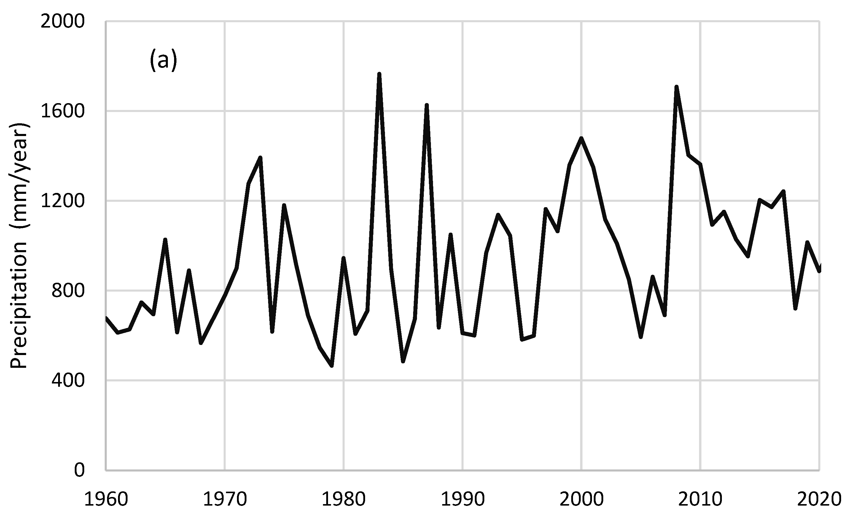
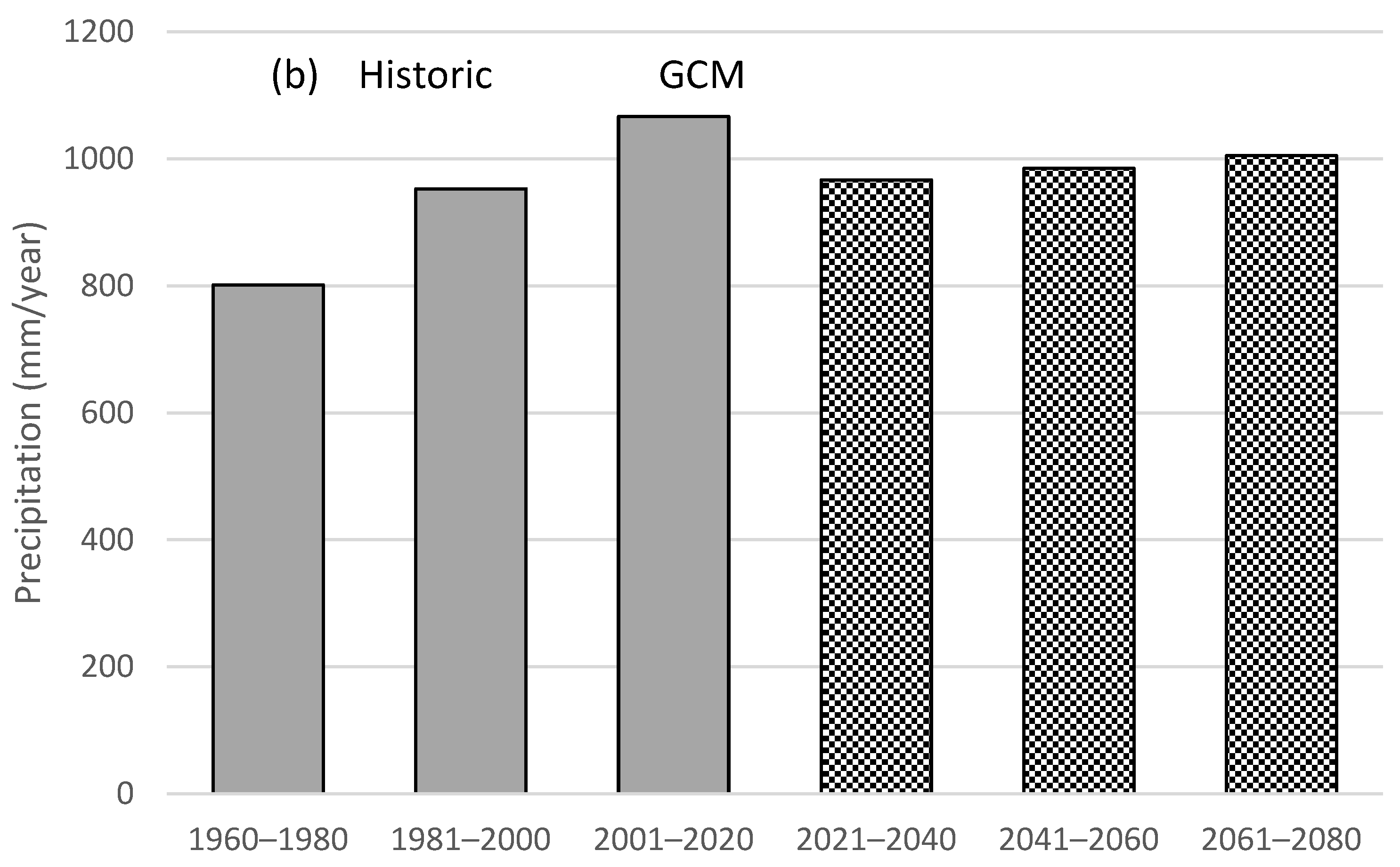
3.4. Annual Precipitation Deficits and Future Projections

Figure 8a is a time series of annual catchment average precipitation for the period 1961–2020 extracted from WorldClim 2.1. High interannual variability is evident, with a strong El Nino influence, particularly in the pre-2000 period. The Hurst coefficient H for the time series is 0.75, reflecting strong LTP. Precipitation has increased consistently over this period; this is shown in Figure 8b which is a plot of 20-year averages for the three historic periods and the three 20-year average GCM projections presented in Table 4 for SSP2-4.5. This increase in precipitation has been observed at the much larger scale of most of the coastal extension of northern South America and Colombia [47]. It might be tempting to attribute this increase in precipitation to anthropogenic climate change. However, an analysis of precipitation deficits for the 8 global regions referred to above and the GPCC gridded data for the period 1900–2020 found no evidence of any increase in deficits across the 8 regions for the 40-year period 1981–2020. Therefore, these deficits continue to be driven primarily by natural climatic variability and associated LTP. Moreover, the observed increase in precipitation shown in Figure 8b may not necessarily continue and may reverse; the GCM average projections show a decrease in the first time window and a slight increase in the subsequent time windows. Different regions may exhibit surplus or deficit precipitation at different times as shown by the cumulative departure from the mean (CDM) plots for the different global regions in O’Connell et al. (2023) [48]. Increasing and decreasing trends for the period 1951–2016 have been observed for different South American regions by da Costa et al. (2024) [47].

Table 5. (a) Durations, standardised percentage volumes, and intensities for precipitation deficits below the mean in each 20-year period; (b) calculation of E(D), E(SV), and E(I) based on the data in (a).

(a)
Period 1 1961–1980								$\overline{X}$ = 807.71
Start			End		D			SV		SI
1962			1964		3			43.82		14.61
1966			1966		1			23.95		23.95
1968			1970		3			50.72		16.91
1974			1974		1			23.61		23.61
1977			1979		3			89.38		29.79
Period 2 1981–2000								$\overline{X}$ = 952.76
Start			End		D			SV		SI
1982			1982		1			25.42		25.42
1984			1986		3			84.43		28.14
1988			1988		1			33.31		33.31
1990			1991		2			72.88		36.44
1995			1996		2			76.08		38.04
Period 3 2001–2020								$\overline{X}$ = 1070.36
Start			End		D			SV		SI
2003			2007		5			126.05		25.21
2013			2014		2			14.91		7.46
2018			2020		3			54.98		18.33
(b)
D	${ND}_i$	$f_i$		E(D)		$\overline{\mathrm{S}\mathrm{V}}$	E(SV)		$\overline{\mathrm{S}\mathrm{I}}$		E(SI)
1	4	0.27		0.27		26.57	7.09		26.57		7.09
2	3	0.24		0.49		54.62	13.35		27.31		6.68
3	5	0.38		1.13		64.67	24.43		21.56		8.14
4	0	0.00		0.00		0.00	0.00		0.00		0.00
5	1	0.11		0.56		126.05	14.01		25.21		2.80
	13	1.00		2.44			58.87				24.71

a lists the durations of deficits below the 20-year means as well as the mean standardised percentage volume and intensity statistics, as defined by Equations (5)–(7), respectively. There are five deficit periods in each of the periods 1961–1980 and 1981–2000 with durations of 1–3 years, and three in the period 2001–2020 with durations of 2–5 years. The largest percentage volume deficit is in the period 2001–2020 with a value of 126.05 for a duration of 5 years, while the largest percentage intensity deficit is in the period 1981–2000 with a value of 38.04 for a duration of 2 years. It depends on the impact of these deficits as to which of these events might be the most difficult to manage in water resources terms.

Table 5b summarises the calculation of $E\left(D\right)$, $E\left(SV\right)$, and $E\left(SI\right)$ based on Equations (8)–(10). The expected duration of a deficit is 2.44 years, while the expected percentage volume and intensity are 58.87 and 24.71, respectively, based on the mean of a 20-year period. These results can therefore be applied to the projected GCM 20-year means based on the assumption that the statistical properties of historical deficits are representative of future deficits. For example, the projected GCM mean for the period 2021–2040 and SPP2-4.5 is 967 mm, so the expected volume and intensity deficits would be 569.27 mm and 238.95 mm, respectively. These are indicative of the highly variable precipitation regimes for the Catamayo catchment, which can be challenging for water resources management. It may be that these deficits will intensify in the future due to anthropogenic climate change, but as already noted above, no evidence of this has been found on average across global regions for recent decades, but it cannot be discounted as anthropogenic climate change is expected to intensify in the future.

To link with water resources applications, the precipitation deficits need to be converted to runoff deficits and impacts on water resources operations assessed from these. This could be done using a runoff coefficient calculated from the average annual precipitation and runoff data for the concurrent period of record. The runoff deficits will have direct implications for the operation of water infrastructure in the Catamayo-Chira catchment in the future. For hydropower generation, extended deficit periods can result in reduced reservoir inflows, lowering water levels and limiting the capacity to generate electricity consistently, particularly during dry seasons when energy demand may remain high. This situation may require increased reliance on alternative energy sources, often at higher operational costs. Similarly, in the agricultural sector, irrigation planning is highly sensitive to the timing and persistence of precipitation and runoff shortfalls. Prolonged deficits during key planting or crop development stages can lead to soil moisture depletion, reduced yields, and increased irrigation water demand—placing additional stress on already limited water resources. Anticipating the frequency and severity of such deficits is therefore crucial for designing more resilient reservoir operation rules and irrigation schedules under future climate conditions.

3.5. Mitigation and Adaptation Strategies

As mentioned in Section 3.3, the results suggest a significant reduction in water availability in the Catamayo catchment, which can have serious consequences for various water uses in the study area, particularly for irrigation and electricity generation.

For irrigation, reduced water availability can lead to lower crop yields, increased competition for water, and the need for costly adaptation measures, such as more efficient irrigation systems or less water-intensive crops. In terms of electricity generation, decreased water flow can reduce hydropower capacity, leading to higher energy costs and increased reliance on fossil fuels, potentially straining existing infrastructure and necessitating new investments.

Mitigation and adaptation strategies include implementing water-saving measures, diversifying energy sources to reduce reliance on hydropower, and adopting integrated water resource management approaches. Developing infrastructure capable of withstanding climate impacts, such as drought-resistant crops and advanced irrigation systems, will be crucial. Addressing these challenges requires a comprehensive, adaptive approach to ensure sustainable water use and minimise adverse effects on agriculture and energy production.

3.6. Limitations and Future Research

There are some limitations to the approach presented in this study. We considered only one downscaling method and a simple hydrological model (a Budyko-based model). While downscaling methods and hydrological models contribute to variability in estimates of climate change impacts, as noted by Chen et al. (2011) [49] and Wilby et al. (1998) [50], these choices were due to this study’s primary focus on investigating the variability related to GCM outcomes, which have been identified as major sources of uncertainty in climate change studies [46]. In comparison, the water balance has been closed to a high level of accuracy by optimising Fu’s parameter $w$, so the dominant source of uncertainty in the water balance is the GCM projections.

Moreover, the variability of climate change impacts may vary among catchments due to differing hydro-climatological characteristics and the interactions between climate simulations and regional conditions [51,52]. It would be beneficial to apply the methodology presented here to other catchments to draw more generalised conclusions.

Furthermore, it is noteworthy that precipitation is the most sensitive variable in estimating water availability (runoff); small changes in mean annual precipitation can lead to significant variations in water availability estimates [53,54]. Although the catchment-wide precipitation estimates based on WorldClim in this study align with those derived from limited local records reported in other studies, there may be lower confidence in these estimates due to the unique topography of the Catamayo catchment. More research in this area is suggested, given that the conclusions of this work rely on accurate estimations of historical values of the water budget components; note that this work compares an 95th percentile band around the estimation of a future value with a historical value considered as the reference, calculated over a 21-year period (1990–2011).

An analysis of GCM projected precipitation time series would allow the properties of precipitation deficits to be estimated directly for future time windows. However, the reproduction of natural long-term persistence by GCMs in future projections has been identified as deficient [55,56,57], which represents an area of concern in assessing the severity of droughts under a future climate [58]. Moreover, Varuolo-Clarke et al. (2022) [59] have noted that the fifth generation European Centre for Medium-Range Weather Forecasting atmospheric reanalysis data, ERA-5, fails to simulate the known southeastern South America precipitation increase from 1951 to 2020, and instead simulates an erroneous precipitation decrease over this period. This outcome demonstrates that adaptation planning based on one expected scenario may not be robust under other scenarios and high uncertainty.

To capture the envelope of uncertainty for future precipitation, a stochastic time series simulation approach could be employed based on the Hurst coefficient/Hurst Kolmogorov dynamics. Multiple possible annual time series of future precipitation can be generated, and a risk assessment of future deficits carried out. For example, this approach proved effective in managing a prolonged drought that affected the water supply of Athens around 1990 [60].

The original Budyko framework and its extension by Fu (1981) [18], while widely used to estimate long-term mean water balance components at large spatial scales, assume steady-state hydrological conditions and negligible changes in water storage over the period considered. These simplifications may limit their applicability, as such conditions are not valid for all catchments globally or at finer temporal and spatial resolutions. Furthermore, although the extension of the Budyko framework employed in this study—proposed by Fu (1981) [18]—introduces a calibratable parameter (ω) to reflect catchment-specific characteristics, it does not explicitly account for dynamic future processes, such as land use change, vegetation dynamics, or human interventions (e.g., irrigation or reservoir operations).

Finally, another limitation of this study relates to the use of the Thornthwaite method for estimating potential evapotranspiration (PET). While Thornthwaite’s approach is advantageous in data-scarce regions due to its minimal input requirements, it is known to underestimate PET in tropical and high-altitude areas—such as the Catamayo catchment—because it relies solely on temperature and does not account for other important climatic drivers such as solar radiation, humidity, and wind speed. This omission can lead to biases in the estimation of PET and, consequently, in the derived aridity index and water balance projections. Although previous studies (e.g., [33]) have shown that various PET formulations tend to yield similar future trends due to the co-dependence of climatic variables, it is important to recognise that differences in magnitude may persist. Therefore, our findings may represent a conservative estimate of future aridity and evapotranspiration increases. Future research should consider implementing more physically based PET models, such as the FAO Penman–Monteith method, provided that sufficient climatic data (e.g., radiation, wind speed, and relative humidity) are available for the region.

4. Conclusions

The climate change impact estimates on the mean annual water balance have been quantified and analysed in a catchment that supplies surface water to two crucial irrigation projects in southern Ecuador and northern Peru, which are vital for the economies of these countries. This impact was assessed using outcomes from 23 Global Circulation Models, GCMs, from the Coupled Model Intercomparison Project—Phase 6, CMIP6, considering the “Middle of the Road” scenario (SSP2-4.5) and the “Fossil Fuel-Driven Development” scenario (SSP8.5). This approach enabled the estimation of a 95th percentile band for each scenario, representing the variability of future projections. It was observed that this variability increases over time for all variables of the mean annual water balance. The results indicate an increase in the aridity in the arid and semi-arid zones of the Catamayo Catchment and a potential reduction in water availability ranging from 26.3 ± 12.3% to 33.3 ± 17%, across the near (2021–2040), mid (2041–2060), and far (2061–2080) future periods, attributable to insignificant change of precipitation depths (statistically speaking) and an increase in actual evapotranspiration.

The climatic regime affecting the catchment is highly variable, and so the water balance analysis has been augmented by an analysis of the statistical properties of historical precipitation deficits. A novel hybrid method has been developed for projecting these results onto the GCM precipitation averages for future periods.

Based on the water balance projections, a reduction in crop yields and hydropower capacity is expected in the study zone in the future, exacerbated by high hydrological variability. This will likely lead to higher energy costs, increased reliance on fossil fuels, and greater competition for water. In this context, it is recommended to implement mitigation measures such as water-saving strategies, diversifying energy sources to reduce reliance on hydropower, and adopting integrated water resource management approaches.

References

1. Yao, L.; Libera, D.A.; Kheimi, M.; Sankarasubramanian, A.; Wang, D. The Roles of Climate Forcing and Its Variability on Streamflow at Daily, Monthly, Annual, and Long-Term Scales. Water Resour. Res. 2020, 56, e2020WR027111. [Google Scholar] [CrossRef]
2. Austin, J.; Zhang, L.; Jones, R.N.; Durack, P.; Dawes, W.; Hairsine, P. Climate Change Impact on Water and Salt Balances: An Assessment of the Impact of Climate Change on Catchment Salt and Water Balances in the Murray-Darling Basin, Australia. Clim. Change 2010, 100, 607–631. [Google Scholar] [CrossRef]
3. Campozano, L.; Ballari, D.; Montenegro, M.; Avilés, A. Future Meteorological Droughts in Ecuador: Decreasing Trends and Associated Spatio-Temporal Features Derived From CMIP5 Models. Front. Earth Sci. 2020, 8, 17. [Google Scholar] [CrossRef]
4. Carvajal, P.E.; Li, F.G.N. Challenges for Hydropower-Based Nationally Determined Contributions: A Case Study for Ecuador. Clim. Policy 2019, 19, 974–987. [Google Scholar] [CrossRef]
5. Zhang, Y.; Engel, B.; Ahiablame, L.; Liu, J. Impacts of Climate Change on Mean Annual Water Balance for Watersheds in Michigan, USA. Water 2015, 7, 3565–3578. [Google Scholar] [CrossRef]
6. Wang, S.; McKenney, D.W.; Shang, J.; Li, J. A National-scale Assessment of Long-term Water Budget Closures for Canada’s Watersheds. J. Geophys. Res. Atmos. 2014, 119, 8712–8725. [Google Scholar] [CrossRef]
7. Han, J.; Yang, Y.; Roderick, M.L.; McVicar, T.R.; Yang, D.; Zhang, S.; Beck, H.E. Assessing the Steady-State Assumption in Water Balance Calculation Across Global Catchments. Water Resour. Res. 2020, 56, e2020WR027392. [Google Scholar] [CrossRef]
8. Collignan, J.; Polcher, J.; Bastin, S.; Quintana-Segui, P. Budyko Framework Based Analysis of the Effect of Climate Change on Watershed Evaporation Efficiency and Its Impact on Discharge Over Europe. Water Resour. Res. 2023, 59, e2023WR034509. [Google Scholar] [CrossRef]
9. Safeeq, M.; Bart, R.R.; Pelak, N.F.; Singh, C.K.; Dralle, D.N.; Hartsough, P.; Wagenbrenner, J.W. How Realistic Are Water-balance Closure Assumptions? A Demonstration from the Southern Sierra Critical Zone Observatory and Kings River Experimental Watersheds. Hydrol. Process. 2021, 35, e14199. [Google Scholar] [CrossRef]
10. Wang, D. Evaluating Interannual Water Storage Changes at Watersheds in Illinois Based on Long-term Soil Moisture and Groundwater Level Data. Water Resour. Res. 2012, 48, W03502. [Google Scholar] [CrossRef]
11. Li, Z.; Li, Q.; Wang, J.; Feng, Y.; Shao, Q. Impacts of Projected Climate Change on Runoff in Upper Reach of Heihe River Basin Using Climate Elasticity Method and GCMs. Sci. Total Environ. 2020, 716, 137072. [Google Scholar] [CrossRef]
12. Osborne, J.M.; Lambert, F.H. A Simple Tool for Refining GCM Water Availability Projections, Applied to Chinese Catchments. Hydrol. Earth Syst. Sci. 2018, 22, 6043–6057. [Google Scholar] [CrossRef]
13. Teng, J.; Chiew, F.H.S.; Vaze, J.; Marvanek, S.; Kirono, D.G.C. Estimation of Climate Change Impact on Mean Annual Runoff across Continental Australia Using Budyko and Fu Equations and Hydrological Models. J. Hydrometeorol. 2012, 13, 1094–1106. [Google Scholar] [CrossRef]
14. Zaninelli, P.G.; Menéndez, C.G.; Falco, M.; López-Franca, N.; Carril, A.F. Future Hydroclimatological Changes in South America Based on an Ensemble of Regional Climate Models. Clim. Dyn. 2019, 52, 819–830. [Google Scholar] [CrossRef]
15. Jaramillo, F.; Piemontese, L.; Berghuijs, W.R.; Wang-Erlandsson, L.; Greve, P.; Wang, Z. Fewer Basins Will Follow Their Budyko Curves Under Global Warming and Fossil-Fueled Development. Water Resour. Res. 2022, 58, e2021WR031825. [Google Scholar] [CrossRef] [PubMed]
16. IPCC Synthesis Report of the Sixth Assessment Report. Available online: https://www.ipcc.ch/ar6-syr/ (accessed on 3 December 2022).
17. Joslyn, S.; Demnitz, R. Communicating Climate Change: Probabilistic Expressions and Concrete Events. Weather Clim. Soc. 2019, 11, 651–664. [Google Scholar] [CrossRef]
18. Fu, B.-P. On the Calculation of the Evaporation from Land Surface. Chin. J. Atmos. Sci. 1981, 5, 23–31. [Google Scholar] [CrossRef]
19. Lavado-Casimiro, W.S.; Felipe, O.; Silvestre, E.; Bourrel, L. ENSO Impact on Hydrology in Peru. Adv. Geosci. 2013, 33, 33–39. [Google Scholar] [CrossRef]
20. Pacheco, J.; Solera, A.; Avilés, A.; Tonón, M.D. Influence of ENSO on Droughts and Vegetation in a High Mountain Equatorial Climate Basin. Atmosphere 2022, 13, 2123. [Google Scholar] [CrossRef]
21. Pineda, L.; Ntegeka, V.; Willems, P. Rainfall Variability Related to Sea Surface Temperature Anomalies in a Pacific–Andean Basin into Ecuador and Peru. Adv. Geosci. 2013, 33, 53–62. [Google Scholar] [CrossRef]
22. Tote, C.; Govers, G.; Van Kerckhoven, S.; Filiberto, I.; Verstraeten, G.; Eerens, H. Effect of ENSO Events on Sediment Production in a Large Coastal Basin in Northern Peru. Earth Surf. Process. Landf. 2011, 36, 1776–1788. [Google Scholar] [CrossRef]
23. Foucher, A.; Morera, S.; Sanchez, M.; Orrillo, J.; Evrard, O. El Niño–Southern Oscillation (ENSO)-Driven Hypersedimentation in the Poechos Reservoir, Northern Peru. Hydrol. Earth Syst. Sci. 2023, 27, 3191–3204. [Google Scholar] [CrossRef]
24. PENUD. Gestión Integrada de Recursos Hídricos de Las Cuencas Transfronterizas y Acuíferos de Puyango-Tumbez, Catamayo-Chira, y Zarumilla; PENUD: Quito, Ecuador, 2015. [Google Scholar]
25. Vílchez, S.; Núñez, S. Valenzuela Germán Estudio Geoambiental de La Cuenca Del Río Chira-Catamayo-[Boletín C 31]; INGEMMET: Lima, Peru, 2006. [Google Scholar]
26. Fick, S.E.; Hijmans, R.J. WorldClim 2: New 1-km Spatial Resolution Climate Surfaces for Global Land Areas. Int. J. Climatol. 2017, 37, 4302–4315. [Google Scholar] [CrossRef]
27. Newell, F.L.; Ausprey, I.J.; Robinson, S.K. Spatiotemporal Climate Variability in the Andes of Northern Peru: Evaluation of Gridded Datasets to Describe Cloud Forest Microclimate and Local Rainfall. Int. J. Climatol. 2022, 42, 5892–5915. [Google Scholar] [CrossRef]
28. Ceccarelli, V.; Fremout, T.; Chavez, E.; Argüello, D.; Loor Solórzano, R.G.; Sotomayor Cantos, I.A.; Thomas, E. Vulnerability to Climate Change of Cultivated and Wild Cacao in Ecuador. Clim. Change 2024, 177, 103. [Google Scholar] [CrossRef]
29. Zhang, L.; Hickel, K.; Dawes, W.R.; Chiew, F.H.S.; Western, A.W.; Briggs, P.R. A Rational Function Approach for Estimating Mean Annual Evapotranspiration. Water Resour. Res. 2004, 40, 2502. [Google Scholar] [CrossRef]
30. Ruggiu, D.; Viola, F. Linking Climate, Basin Morphology and Vegetation Characteristics to Fu’s Parameter in Data Poor Conditions. Water 2019, 11, 2333. [Google Scholar] [CrossRef]
31. Ning, T.; Li, Z.; Feng, Q.; Liu, W.; Li, Z. Comparison of the Effectiveness of Four Budyko-Based Methods in Attributing Long-Term Changes in Actual Evapotranspiration. Sci. Rep. 2018, 8, 12665. [Google Scholar] [CrossRef]
32. Aschonitis, V.; Touloumidis, D.; ten Veldhuis, M.-C.; Coenders-Gerrits, M. Correcting Thornthwaite Potential Evapotranspiration Using a Global Grid of Local Coefficients to Support Temperature-Based Estimations of Reference Evapotranspiration and Aridity Indices. Earth Syst. Sci. Data 2022, 14, 163–177. [Google Scholar] [CrossRef]
33. Lemaitre-Basset, T.; Oudin, L.; Thirel, G.; Collet, L. Unraveling the Contribution of Potential Evaporation Formulation to Uncertainty under Climate Change. Hydrol. Earth Syst. Sci. 2022, 26, 2147–2159. [Google Scholar] [CrossRef]
34. Mather, J.R.; Ambroziak, R.A. A Search for Understanding Potential Evapotranspiration. Geogr. Rev. 1986, 76, 355. [Google Scholar] [CrossRef]
35. Almazroui, M.; Ashfaq, M.; Islam, M.N.; Rashid, I.U.; Kamil, S.; Abid, M.A.; O’Brien, E.; Ismail, M.; Reboita, M.S.; Sörensson, A.A.; et al. Assessment of CMIP6 Performance and Projected Temperature and Precipitation Changes Over South America. Earth Syst. Environ. 2021, 5, 155–183. [Google Scholar] [CrossRef]
36. Schneider, U.; Becker, A.; Finger, P.; Meyer-Christoffer, A.; Rudolf, B.; Ziese, M. GPCC Full Data Reanalysis Version 7.0 at 0.5°: Monthly Land-Surface Precipitation from Rain-Gauges Built on GTS-Based and Historic Data. Available online: https://opendata.dwd.de/climate_environment/GPCC/html/fulldata_v7_doi_download.html (accessed on 5 March 2024).
37. O’Connell, E.; O’Donnell, G.; Koutsoyiannis, D. The Spatial Scale Dependence of The Hurst Coefficient in Global Annual Precipitation Data, and Its Role in Characterising Regional Precipitation Deficits within a Naturally Changing Climate. Hydrology 2022, 9, 199. [Google Scholar] [CrossRef]
38. Santos, F.; Jara, J.; Acosta, N.; Galeas, R.; de Bièvre, B. Assessing Annual and Monthly Precipitation Anomalies in Ecuador Bioregions Using WorldClim CMIP6 GCM Ensemble Projections and Dynamic Time Warping. Int. J. Climatol. 2024, 45, e8685. [Google Scholar] [CrossRef]
39. Ochoa, P.A.; Fries, A.; Mejía, D.; Burneo, J.I.; Ruíz-Sinoga, J.D.; Cerdà, A. Effects of Climate, Land Cover and Topography on Soil Erosion Risk in a Semiarid Basin of the Andes. Catena 2016, 140, 31–42. [Google Scholar] [CrossRef]
40. Ekstrand, S.; Mancinelli, C.; Houghton-Carr, H.; Govers, G.; Debels, P.; Camaño, B.; Alcoz, S.; Filiberto, I.; Gámez, S.; Duque, A. TWINLATIN: Twinning European and Latin American River Basins for Research Enabling Sustainable Water Resources Management. Final Report; IVL Swedish Environmental Research Institute: Stockholm, Sweden, 2009. [Google Scholar]
41. Zhou, G.; Wei, X.; Chen, X.; Zhou, P.; Liu, X.; Xiao, Y.; Sun, G.; Scott, D.F.; Zhou, S.; Han, L.; et al. Global Pattern for the Effect of Climate and Land Cover on Water Yield. Nat. Commun. 2015, 6, 5918. [Google Scholar] [CrossRef]
42. Reaver, N.G.F.; Kaplan, D.A.; Klammler, H.; Jawitz, J.W. Theoretical and Empirical Evidence against the Budyko Catchment Trajectory Conjecture. Hydrol. Earth Syst. Sci. 2022, 26, 1507–1525. [Google Scholar] [CrossRef]
43. Ponce, V.M.; Pandey, R.P.; Ercan, S. Characterization of Drought across Climatic Spectrum. J. Hydrol. Eng. 2000, 5, 222–224. [Google Scholar] [CrossRef]
44. Hu, K.; Huang, G.; Huang, P.; Kosaka, Y.; Xie, S.-P. Intensification of El Niño-Induced Atmospheric Anomalies under Greenhouse Warming. Nat. Geosci. 2021, 14, 377–382. [Google Scholar] [CrossRef]
45. Hou, M.; Tang, Y. Recent Progress in Simulating Two Types of ENSO—From CMIP5 to CMIP6. Front. Mar. Sci. 2022, 9, 986780. [Google Scholar] [CrossRef]
46. Shen, M.; Chen, J.; Zhuan, M.; Chen, H.; Xu, C.-Y.; Xiong, L. Estimating Uncertainty and Its Temporal Variation Related to Global Climate Models in Quantifying Climate Change Impacts on Hydrology. J. Hydrol. 2018, 556, 10–24. [Google Scholar] [CrossRef]
47. da Costa, J.A.C.; Andreoli, R.V.; Kayano, M.T.; de Souza, I.P.; de Souza, R.A.F.; Cerón, W.L. The South American Precipitation Trends under (or Not) El Niño-Southern Oscillation Influences and Relationship with Large-scale Circulation. Int. J. Climatol. 2024, 44, 3154–3168. [Google Scholar] [CrossRef]
48. O’Connell, E.; O’Donnell, G.; Koutsoyiannis, D. On the Spatial Scale Dependence of Long-Term Persistence in Global Annual Precipitation Data and the Hurst Phenomenon. Water Resour. Res. 2023, 59, e2022WR033133. [Google Scholar] [CrossRef]
49. Chen, J.; Brissette, F.P.; Poulin, A.; Leconte, R. Overall Uncertainty Study of the Hydrological Impacts of Climate Change for a Canadian Watershed. Water Resour. Res. 2011, 47, W12509. [Google Scholar] [CrossRef]
50. Wilby, R.L.; Hassan, H.; Hanaki, K. Statistical Downscaling of Hydrometeorological Variables Using General Circulation Model Output. J. Hydrol. 1998, 205, 1–19. [Google Scholar] [CrossRef]
51. Jung, I.-W.; Moradkhani, H.; Chang, H. Uncertainty Assessment of Climate Change Impacts for Hydrologically Distinct River Basins. J. Hydrol. 2012, 466, 73–87. [Google Scholar] [CrossRef]
52. Kay, A.L.; Davies, H.N.; Bell, V.A.; Jones, R.G. Comparison of Uncertainty Sources for Climate Change Impacts: Flood Frequency in England. Clim. Change 2009, 92, 41–63. [Google Scholar] [CrossRef]
53. Hamel, P.; Guswa, A.J. Uncertainty Analysis of a Spatially Explicit Annual Water-Balance Model: Case Study of the Cape Fear Basin, North Carolina. Hydrol. Earth Syst. Sci. 2015, 19, 839–853. [Google Scholar] [CrossRef]
54. Redhead, J.W.; Stratford, C.; Sharps, K.; Jones, L.; Ziv, G.; Clarke, D.; Oliver, T.H.; Bullock, J.M. Empirical Validation of the InVEST Water Yield Ecosystem Service Model at a National Scale. Sci. Total Environ. 2016, 569–570, 1418–1426. [Google Scholar] [CrossRef]
55. Koutsoyiannis, D.; Efstratiadis, A.; Mamassis, N.; Christofides, A. On the Credibility of Climate Predictions. Hydrol. Sci. J. 2008, 53, 671–684. [Google Scholar] [CrossRef]
56. Rocheta, E.; Sugiyanto, M.; Johnson, F.; Evans, J.; Sharma, A. How Well Do General Circulation Models Represent Low-frequency Rainfall Variability? Water Resour. Res. 2014, 50, 2108–2123. [Google Scholar] [CrossRef]
57. Moon, H.; Gudmundsson, L.; Seneviratne, S.I. Drought Persistence Errors in Global Climate Models. J. Geophys. Res. Atmos. 2018, 123, 3483–3496. [Google Scholar] [CrossRef] [PubMed]
58. Ault, T.R.; Cole, J.E.; Overpeck, J.T.; Pederson, G.T.; Meko, D.M. Assessing the Risk of Persistent Drought Using Climate Model Simulations and Paleoclimate Data. J. Clim. 2014, 27, 7529–7549. [Google Scholar] [CrossRef]
59. Varuolo-Clarke, A.M.; Williams, A.P.; Smerdon, J.E.; Ting, M.; Bishop, D.A. Influence of the South American Low-Level Jet on the Austral Summer Precipitation Trend in Southeastern South America. Geophys. Res. Lett. 2022, 49, e2021GL096409. [Google Scholar] [CrossRef]
60. Koutsoyiannis, D. Hurst-Kolmogorov Dynamics and Uncertainty1. JAWRA J. Am. Water Resour. Assoc. 2011, 47, 481–495. [Google Scholar] [CrossRef]
Figure 1. Location of the study catchment.
Hydrology 12 00177 g001
Figure 2. Illustration of the framework used in this work.
Hydrology 12 00177 g002
Figure 3. Illustration of the Budyko space and interannual variability of the aridity index and evapotranspiration rate (black points); the average value is represented by the red point. Arrows represent potential movements of the points due to climate change.
Hydrology 12 00177 g003
Figure 4. Historical 5 km grid values and future projections of mean annual precipitation, temperature and potential evapotranspiration for the far future (2061–2080).
Hydrology 12 00177 g004
Figure 5. Historical values of the long-term average actual evapotranspiration rate and aridity index alongside future projections, computed as the mean of (23) GCM outcomes using Fu’s equation (Equation (2)). The vertical and horizontal lines on these points indicate the 95% confidence intervals for these indices derived from these outcomes.
Hydrology 12 00177 g005
Figure 6. Historical average monthly precipitation and potential evapotranspiration values, future estimates and their confidence bands.
Hydrology 12 00177 g006
Figure 7. Mean annual water balance variables, future projections, and their confidence bands.
Hydrology 12 00177 g007
Figure 8. (a) Annual catchment average precipitation for the period 1961–2020. (b) Twenty-year mean precipitation for historic periods 1961–1980, 1981–2000 and 2001–2020, and GCM projections for 2021-40, 2041-60 and 2061-80 based on the CMIP6′s SSP2-4.5.
Hydrology 12 00177 g008aHydrology 12 00177 g008b