Tail-Aware Forecasting of Precipitation Extremes Using STL-GEV and LSTM Neural Networks

Abstract

Accurate prediction of extreme precipitation events remains a critical challenge in hydrological forecasting due to their rare occurrence and complex statistical behavior. These extreme events are becoming more frequent and intense under the influence of climate change. Their unpredictability not only hampers water resource management and disaster preparedness but also leads to disproportionate impacts on vulnerable communities and critical infrastructure. Therefore, in this article, we introduce a hybrid modeling framework that combines Generalized Extreme Value (GEV) distribution fitting with deep learning models to forecast monthly maximum precipitation extremes. Long Short-term Memory models (LSTMs) are proposed to predict the cumulative distribution (CDF) values of the GEV-fitted remainder series. This approach transforms the forecasting problem into a bounded probabilistic learning task, improving model stability and interpretability. Crucially, a tail-weighted loss function is designed to emphasize rare but high-impact events in the training process, addressing the inherent class imbalance in extreme precipitation predictions. Results demonstrate strong predictive performance in both the CDF and residual domains, with the proposed model accurately identifying anomalously high precipitation months. This hybrid GEV–deep learning approach offers a promising solution for early warning systems and long-term climate resilience planning in hydrologically sensitive regions.

1. Introduction

The frequency, intensity, and distribution of extreme precipitation events have been undergoing significant changes globally, including notable trends observed throughout the United States [1,2,3]. Numerous regions across the globe have already experienced and continue to grapple with intensified extreme weather events, especially flooding triggered by severe rainfall [4,5]. Texas, specifically, represents a region characterized by considerable variability in annual precipitation totals and faces projections that indicate an increased frequency and intensity of extreme precipitation events in the coming decades [6,7]. This anticipated shift translates directly into heightened flood risks, presenting multifaceted challenges for infrastructure, urban planning, and disaster response strategies. Extreme precipitation events often exceed the designed capacity and resilience thresholds of existing physical infrastructure systems, including drainage networks and flood management structures. Such exceedances can rapidly lead to systemic failures when infrastructure cannot adequately accommodate the volume and intensity of rainfall [8,9,10,11]. In urban environments, the consequences of surpassing drainage capacities manifest through stormwater flooding, causing cascading impacts across multiple critical sectors. These impacts commonly include severe traffic congestion, transportation disruptions, heightened safety hazards for communities, impediments to timely emergency response operations, complex logistical challenges in resource allocation, and recovery efforts following such disruptive events. Consequently, advancing research focused on accurately forecasting and effectively predicting extreme precipitation events has become increasingly essential for improving preparedness, resilience, and adaptive capacity across hydrologically vulnerable regions [12].

Accurate prediction of extreme precipitation events is a major challenge in forecasting due to their rare occurrence and complex behavior [13,14]. Monthly and seasonal precipitation totals have been predicted with relatively good accuracy from dynamically downscaled climate model ensembles, and when combined with bias correction techniques, accuracy has improved in predicting extreme precipitation [15,16,17]. However, dynamically downscaled models require a large amount of time and computational resources to develop and run, which is where statistical methods have shown to be an advantage by addressing these limitations [9,18,19]. While traditional deep learning methods have shown promise in general time series tasks [20], they often struggle with extremes because they typically rely on conventional quadratic loss functions that underemphasize outliers. To address this limitation, Ding et al. proposed a novel approach incorporating a memory network to retain information about past extreme events [21]. By integrating a specialized Extreme Value Loss (EVL) function with an adapted memory network, they developed an end-to-end framework capable of improving prediction accuracy for rare and impactful events. In the context of precipitation forecasting, numerous studies have explored both short- and long-term prediction strategies [17,19,22]. For short-term forecasting, Sønderby et al. introduced MetNet, a deep neural network designed to predict precipitation up to 8 h ahead at a spatial resolution of 1 km² and a temporal resolution of 2 min [23]. MetNet demonstrated state-of-the-art performance, outperforming traditional Numerical Weather Prediction (NWP) models across the continental United States for forecasts extending up to 7–8 h. In another study by Lin et al., Convolutional Neural Networks (CNNs) with a space-based attention mechanism improved the predictive accuracy of 12 and 6 h extreme rainfall when observed rainfall values were included in the model [24]. For longer-term and extreme event forecasting, recent work has explored hybrid and attention-based architectures. For example, Luo et al. proposed the LSTM-SelfAttention model, which combined Long Short-Term Memory (LSTM) networks with self-attention mechanisms to capture long-term dependencies and highlight salient features in time series data [25]. Using precipitation records from Kunming between 1961 and 2020, their model achieved a 28% improvement in accuracy compared to a conventional backpropagation neural network. Similarly, Liu et al. [26] applied an LSTM-based model to forecast monthly precipitation over the Qinghai–Tibet Plateau from 1990 to 2016. Their results showed that the LSTM improved the average coefficient of determination (R²) by 0.07 and 0.36 compared to traditional Recurrent Neural Network (RNN) and AutoRegressive Integrated Moving Average (ARIMA) models, respectively.

Despite these advances, existing models often remain limited in their ability to represent the distributional properties of extremes. Most frameworks are optimized for average-case performance, with limited attention given to tail-specific accuracy or distributional robustness. Moreover, relatively few studies combine statistical extreme value theory with deep learning in a unified forecasting pipeline. To address these gaps, this study proposes a hybrid modeling framework that integrates traditional statistical decomposition, Generalized Extreme Value (GEV)-based probabilistic transformation, and tail-aware deep learning. First, the original precipitation time series is decomposed using seasonal trend decomposition based on Loess (STL), isolating the trend, seasonality, and irregular remainder components. The remainder series, which contains most of the extreme variation, is fitted with a GEV distribution and transformed into cumulative distribution function (CDF) values. This transforms the forecasting problem into a bounded probabilistic learning task. An LSTM neural network is then trained to predict the GEV-transformed series using a custom tail-weighted loss function, which emphasizes learning from high-impact events. This hybrid framework combines the interpretability of statistical modeling with the representational power of deep learning, making it well-suited for forecasting rare and impactful precipitation extremes. Similarly, the decomposition method was applied in [27]. Wang et al. proposed a novel forecasting model SSA-BiTCN-SelfAttention to address the nonlinear and nonstationary characteristics of runoff sequences in hydrological prediction. The model integrated Singular Spectrum Analysis (SSA) [28], Bi-directional Temporal Convolutional Network (BiTCN) [29], and a Self-Attention mechanism. SSA was applied to decompose and reconstruct runoff data, reducing noise and highlighting key periodic and trend information. The reconstructed sequences were then modeled using BiTCN with bi-directional training, while the Self-Attention mechanism captured long-range dependencies to further enhance predictive performance.

In general, the objectives and contributions of this study are to develop a deep learning-based framework for forecasting monthly maximum extreme precipitation by integrating statistical decomposition and GEV modeling with neural network learning. The major components are as follows: (1.) use of STL decomposition to separate trend, seasonality, and remainder components from the precipitation time series; (2.) application of GEV distribution to model and transform the residual series into a probabilistic domain; (3.) design and tuning of a tail-aware LSTM using a custom loss function to enhance prediction of rare events; and (4.) comprehensive evaluation using Peak Over Threshold (POT) metrics to assess extreme event forecasting performance. The rest of the manuscript is organized as follows: Section 2 presents the data pre-processing steps, STL decomposition, and GEV-based transformation of the remainder series. It introduces the design of the tail-weighted LSTM and explains the hyperparameter tuning approach using Keras Tuner. Section 3 reports experimental results and performance comparisons, focusing on both general accuracy and the ability to capture extremes. Finally, Section 4 concludes the study, highlighting the model’s strengths, limitations, and potential applications in hydrological forecasting.

2. Materials and Methods

2.1. Data Source

Observational precipitation data for bias correction of projected values were obtained from the Automated Surface Observing System (ASOS), which operates continuously, providing weather measurements 24 h a day. This study specifically utilized 24 h time series data, acquired from the Iowa Environmental Mesonet maintained by Iowa State University [30]. For analysis, multiple weather stations located in the Dallas–Fort Worth, Texas, area were selected, including ‘ADS’, ‘DAL’, ‘RBD’, ‘LNC’, ‘DFW’, ‘GPM’, ‘GKY’, ‘HQZ’, ‘TKI’, ‘FTW’, ‘AFW’, ‘NFW’, ‘FWS’, ‘DTO’, and ‘JWY’ (Figure 1). Additionally, two weather stations from the Houston, Texas, area (‘HOU’ and ‘IAH’) and one from El Paso, Texas (‘ELP’), were included. In this study, the proposed methods were applied to all selected weather stations across Texas. However, for clarity and conciseness, illustrative figures presented in the article focus on the Red Bird Executive Airport (RBD) station, which is situated in the Five Mile Creek watershed and lies within the administrative boundary of the city of Dallas. The RBD station has maintained precipitation records since January 1, 1997, with measurements originally recorded at 5 min intervals.

2.2. Data Processing

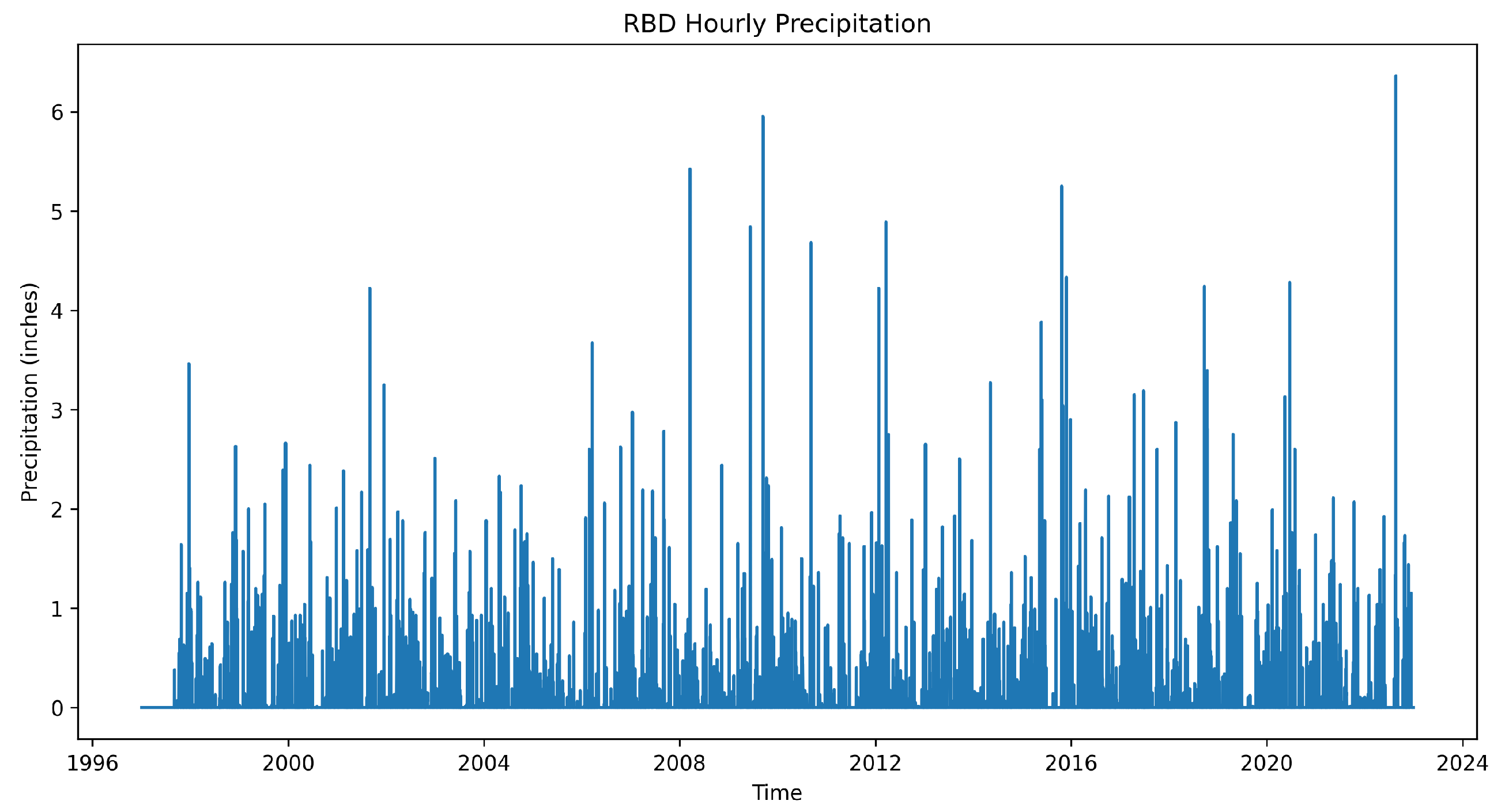
The original precipitation dataset was recorded at irregular time intervals, capturing cumulative precipitation values at sub-hourly timestamps. To derive a consistent hourly precipitation dataset suitable for analysis, the original data were first converted into a uniformly spaced hourly series through resampling. Given that the data represent cumulative precipitation recorded over varying intervals within each hour, the maximum precipitation value observed within each hourly interval was selected to represent the maximum precipitation intensity for that hour. Specifically, the .resample(‘H’).max() method was employed, which aggregates the data by hour and assigns the maximum oberserved precipitation value to each hourly period. Missing hourly intervals with no recorded precipitation values were filled with zeros using .fillna(0) to ensure the continuity and completeness of the dataset. This procedure resulted in reliable and uniformly spaced hourly precipitation data suitable for subsequent analysis and modeling. Figure 2 is a demonstration for the hourly precipitation dataset of the weather station at RBD.

To facilitate the analysis of precipitation extremes at broader temporal scales, the hourly dataset was further aggregated. First, daily precipitation totals were obtained by resampling the hourly dataset using the .resample(‘D’).sum() method, which computes the sum of hourly values for each calendar day, thereby capturing the total daily precipitation. This daily aggregation provides a comprehensive view of rainfall distribution over time, smoothing out short-term fluctuations. Next, in order to focus on monthly extremes, the daily dataset was resampled to a monthly scale using the .resample(‘M’).max() method. This operation selects the highest daily precipitation value within each month, effectively identifying the most intense rainfall events on a monthly basis. This approach ensures that monthly extremes are preserved for subsequent statistical modeling and extreme value analysis, which are particularly sensitive to the peak events rather than averages or totals. For STL decomposition, a fixed seasonal period of 12 months was applied uniformly across all weather stations. This choice reflects the dominant annual cycle observed in Texas precipitation patterns, where variability is largely governed by seasonally recurring meteorological drivers. Using a 12-month period ensures that key seasonal signals, such as summer monsoonal influences or winter frontal systems, are properly isolated from the trend and remainder components. Furthermore, applying a consistent seasonal window across all stations provides a standardized basis for downstream analysis, particularly when comparing the behavior of extremes across different geographic locations.

To prepare the dataset for training and testing the deep learning models, a series of pre-processing steps were applied to the GEV-transformed remainder series (expressed in CDF values). First, the time series was split into training and testing subsets using an 80/20 split. Specifically, 80% of the data were allocated for training, and the remaining 20% were reserved for testing, based on the total number of monthly observations. This ensured that the model was trained on historical patterns while being evaluated on unseen future data. Next, a sliding window approach was used to create input–output pairs from the CDF-transformed series. Using a fixed lag of 50 time steps, the model was configured to take the previous 50 CDF values as input and predict the next CDF value as output. This windowing process captured temporal dependencies and local patterns necessary for sequential modeling.

2.3. The Proposed Methods and Models

In this study, the seasonal trend decomposition using Loess (STL) method was employed to analyze the precipitation time series. Originally developed by Cleveland et al. [31], STL is a flexible approach for modeling nonlinear relationships in time series data. It offers several advantages over traditional decomposition methods such as SEATS (Seasonal Extraction in ARIMA Time Series) and X-11 [32]. Unlike SEATS and X-11, which are limited to monthly or quarterly data, STL can accommodate any type of seasonality. Furthermore, it allows the seasonal component to evolve over time, with user-defined control over the rate of change. The method also enables user customization of trend cycle smoothness. An additional strength of STL is its robustness to outliers when robust decomposition is specified; unusual observations have minimal influence on the estimated trend and seasonal components [33].

The Particle Swarm Optimization (PSO) is a population-based metaheuristic algorithm inspired by the social behavior of birds flocking or fish schooling. Introduced by Kennedy and Eberhart in 1995 [34], PSO simulates a swarm of particles that explore the search space by updating their positions based on both their personal best experiences and the experiences of neighboring particles. Each particle adjusts its velocity and position using a combination of inertia, cognitive (personal best), and social (global best) components, allowing the swarm to converge toward optimal or near-optimal solutions efficiently. PSO has been widely applied in various optimization problems due to its simplicity, ease of implementation, and ability to handle nonlinear, non-differentiable objective functions [35]. Over time, several enhancements have been proposed, such as the introduction of constriction coefficients to improve convergence stability. More details on the foundational work of PSO can be found in the original paper [34].

In this part of the study, the goal is to estimate the optimal parameters (location, scale, and shape) of the GEV distribution for the training portion of the remainder series, data that have already been seasonally and trend-wise decomposed. The GevEstimate.psoMethod() function is employed for this purpose, leveraging PSO as a robust global optimization strategy. The remainder series, which captures the irregular and extreme components of precipitation after STL decomposition, serves as the target dataset for fitting. To initialize the PSO algorithm, Pso.computeInitialPos() is used to generate a swarm of 200 particles, each representing a candidate solution in the 3-dimensional GEV parameter space, location, scale, and shape. The specified search ranges for these parameters are set to ensure coverage of plausible values: (−10, 10) for location and shape, and (5, 30) for the scale parameter, which must remain positive. By applying PSO with 200 iterations, the algorithm iteratively refines the swarm’s positions to minimize the negative log-likelihood function of the GEV fit. This approach is particularly advantageous because the GEV likelihood surface can be highly non-convex and sensitive to initial conditions. PSO helps avoid local minima and ensures convergence to a globally optimal set of parameters.

The proposed model is a custom LSTM architecture designed to forecast extreme precipitation behavior from GEV-transformed time series data. To optimize the model’s architecture and training configuration, the Keras Tuner framework was employed for automated hyperparameter tuning. The model accepts an input sequence of 50 time steps and dynamically adjusts its structure based on hyperparameter selections. It can include one or two LSTM layers depending on the value of the use_second_lstm flag, with tunable LSTM units ranging from 32 to 128 in the first layer and 32 to 64 in the second. A dropout layer is used for regularization, with dropout rates selected from the range of 0.1 to 0.5. The dense layer configuration is also tunable, with units ranging from 16 to 64, and with ReLU activation.

A key innovation of the model is the use of a custom tail-weighted loss function (Equation (1)), make_tail_weighted_mse, which emphasizes accurate learning of rare and extreme events by applying increased loss weights to outliers. The loss function is further parameterized by tunable alpha and power values, enabling fine control over how aggressively the model penalizes deviations in the tails. Additionally, the optimizer is configured with an exponentially decaying learning rate, with the initial rate and decay parameters determined during tuning. This integration of domain-specific loss, architectural flexibility, and adaptive training scheduling allows the model to be both expressive and sensitive to the challenges of extreme value forecasting. The hyperparameter tuning process ensures that the final model configuration is well-suited to capturing the temporal and statistical nuances of precipitation extremes.

2.4. Model Evaluation Metrics

In this study, the authors customized a make_tail_weighted_mse function to emphasize prediction accuracy for extreme values in the target distribution, which is particularly important in forecasting rare but impactful events like extreme precipitation. Traditional mean squared error (MSE) treats all errors equally, which can lead to models that perform well on the majority of “normal” cases but poorly on the tails of the distribution, where extremes occur. In the make_tail_weighted_mse function, a weighting factor is introduced using an exponential function:

$$\mathcal{L}(y,\widehat{y})={\displaystyle \frac{1}{n}}\sum _{i=1}^n\left[\alpha ·{\left|y_i-0.5\right|}^p·{(y_i-{\widehat{y}}_i)}^2\right].$$

(1)

where n is the total number of samples in the batch or dataset over which the loss is computed. i is the index of the sample in the sequence from 1 to n, used in summation. $y_i$ is the true value of the target at index i. $\widehat{y}$ is the predicted value produced by the model for the i-th time step. In the tail-weighted MSE loss function, two hyperparameters, $\alpha$ and p, control the degree of emphasis placed on extreme values. The parameter $\alpha$ is a positive scaling factor that amplifies the contribution of samples located further from the center of the distribution (i.e., the median, assumed to be 0.5 in the normalized CDF space). A higher value of $\alpha$ increases the penalty for errors associated with rare or extreme events. The exponent p determines the sensitivity of the weighting scheme to deviations from the center. When $p=1$, the weights increase linearly with the distance from 0.5, whereas higher values of p produce a more aggressive, nonlinear increase in weights, concentrating the learning effort more heavily on the tails. To avoid manual selection and ensure that the model is optimally tuned for each dataset, we integrated these parameters into the Keras Tuner hyperparameter search process, allowing the tuner to explore combinations of these values along with model architecture and training parameters. The selected values were those that minimized mean absolute error (MAE) over the tuning trials. This approach provided a data-driven mechanism for determining the most appropriate loss shaping based on the distribution of each station’s precipitation extremes. As a result, the model was penalized more heavily for errors associated with very high or very low target values, effectively pushing it to focus more on accurately learning the tail behavior of the distribution. This is especially valuable in hydrological modeling, where extreme precipitation events are rare but crucial for risk assessment and planning. By using make_tail_weighted_mse, the model becomes more sensitive to these extreme cases and better suited for applications like early warning systems and resilience planning.

In this study, MSE was used as a primary evaluation and training metric for a fully connected feedforward neural network, implemented using TensorFlow’s built-in tf.losses.MeanSquaredError() function. MSE computes the average of the squared differences between the predicted and actual values, making it a standard and effective metric for assessing the overall accuracy of regression models. Its formulation inherently penalizes larger errors more than smaller ones, encouraging the model to reduce significant deviations and better approximate the central trend of the target distribution. In the context of the trend forecasting models, feedforward neural networks were constructed using multiple dense layers and compiled with the MSE loss function. During training, the model minimized this loss by adjusting its weights through backpropagation, guided by the Adam optimizer with an exponentially decaying learning rate. By minimizing MSE, the model aimed to accurately reconstruct the smooth, low-frequency trend or seasonality component of the precipitation time series while maintaining stability and generalization across different time windows.

To evaluate the hybrid model’s final performance in forecasting extreme precipitation events, POT analysis was employed as a targeted evaluation metric. This method involves defining a quantile threshold based on the distribution of the observed precipitation data. Any event exceeding this threshold is classified as extreme [36]. The model’s predictions are then assessed by computing precision, recall, and F1-score with respect to these extreme cases. Precision reflects the proportion of predicted extremes that are actually extreme, while recall measures the proportion of true extremes that the model successfully identifies. The F1-score provides a harmonic mean of precision and recall, offering a balanced view of the model’s ability to detect rare high-impact events. This approach offers a focused assessment of the model’s effectiveness in identifying and distinguishing extremes, which is especially important in hydrological applications where accurately predicting rare but severe precipitation events is critical for risk mitigation and early warning systems.

3. Results and Discussion

3.1. The STL Decomposition Performance

As mentioned earlier in the article, to focus on monthly extremes, the authors selected the highest daily precipitation value within each month to identify the most intense rain events monthly. Figure 3 displays the monthly maximum precipitation observed at the RBD weather station. The time series spans from the late 1990s to 2023 and captures significant variability in peak daily rainfall on a monthly basis. While most monthly maxima fall between 0 and 3 inches (1 inch is 25.4 mm), several months exhibit extreme peaks, with precipitation exceeding 5 or even 6 inches. These spikes indicate high-intensity rainfall events that can contribute to urban flooding and infrastructure stress. The variability and clustering of extremes in certain periods also suggest underlying seasonal or multi-year climatic influences, highlighting the importance of using tailored statistical models for analyzing and forecasting such extremes.

To prepare the monthly maximum precipitation series for modeling, a seasonal trend decomposition was performed using the STL method. The full dataset was first split into training and testing subsets, with 80% allocated for training and the remaining 20% reserved for evaluation. STL decomposition was then applied to the full monthly time series using the StlDecompose.decompose() function. The input data were reshaped to a 2D array format, and the decomposition was configured with a seasonal period of 12 months to reflect annual cyclic patterns. This process separated the original time series into three additive components: the long-term trend (trend_series), the recurring seasonal pattern (seasonality_series), and the residual or irregular component (remainder_series). The remainder series, in particular, retains the unpredictable, extreme variations in precipitation and serves as the focus for subsequent extreme value modeling and forecasting (Figure 4).

Figure 4 presents the results of STL decomposition applied to the monthly maximum precipitation time series. The top panel shows the trend component, which captures the long-term, low-frequency variations in precipitation intensity over the observed period. While the trend exhibits some multi-decadal fluctuations, it generally reflects the slow-changing baseline around which seasonal and irregular variations occur. The middle panel displays the seasonality component, which captures the recurring annual cycles in the data. This component clearly reveals a consistent seasonal pattern, although its amplitude appears to vary slightly over time—suggesting potential changes in seasonal behavior. The bottom panel illustrates the remainder (or residual) component, which contains the unpredictable and irregular fluctuations not explained by the trend or seasonality. The Augmented Dickey–Fuller (ADF) test for the 18 select stations that are also highlighted in Figure 1 shows that the stationary assumption prevails, or the null hypothesis is rejected, in all tests, with an average ADF statistic of −13.75 compared to critical values at 1%, with the average being equal to −3.45. This component is especially important for modeling extreme precipitation events, as it preserves the sharp spikes and anomalies indicative of high-impact, short-duration rainfall episodes. Together, these components offer a clear separation of systematic patterns and extreme behaviors within the precipitation time series, forming the basis for more accurate and interpretable forecasting models.

3.2. Parameter Estimation of GEV Fitted to Remainder Series

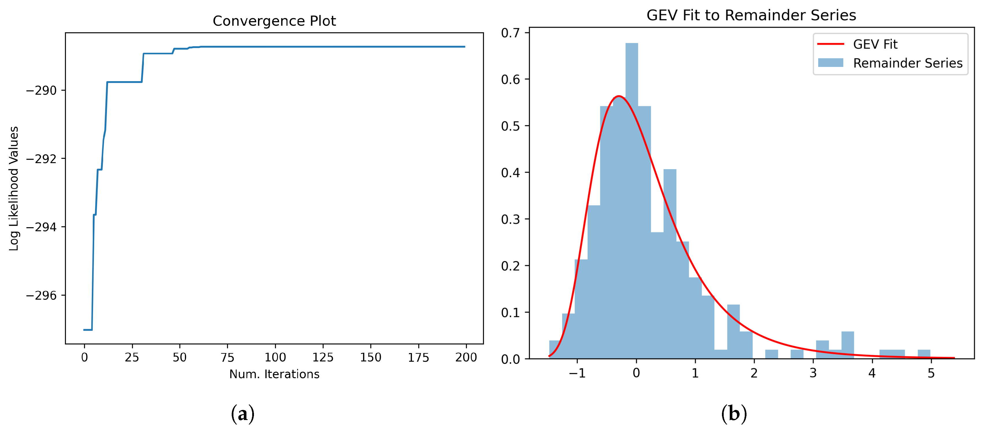
Following the STL decomposition of the monthly maximum precipitation time series, the authors fitted a GEV distribution to the remainder series in order to capture the statistical characteristics of extreme deviations not explained by trend or seasonality. To estimate the GEV parameters, shape, location, and scale, we employed the PSO approach due to its robustness in navigating non-convex likelihood surfaces. Specifically, we used the Pso.computeInitialPos() function to initialize 200 particles within a defined search space for each parameter: [−2, 2] for shape and location, and [0.1, 10] for scale. The optimization was run for 200 iterations to maximize the log-likelihood function of the GEV distribution. The estimated parameters yielded a shape of 0.088, a location of −0.238, and a scale of 0.655, with a maximum log-likelihood value of −288.733. Figure shows the convergence behavior of the PSO algorithm, where the log-likelihood values stabilize within the first 60 iterations, indicating rapid and stable convergence to an optimal solution (Figure 5a). A total of 200 iterations was used to ensure general applicability across all weather stations, as some datasets may require a longer optimization horizon to achieve convergence.

Figure 5 shows the fitted GEV distribution overlaid on the histogram of the STL-decomposed remainder series, representing the residual component of monthly maximum precipitation after trend and seasonal effects have been removed. The histogram reflects the empirical distribution of the training subset of the remainder series, capturing the variability and skewness of extreme precipitation anomalies. The red curve illustrates the probability density function (PDF) of the GEV distribution, parameterized using the optimal values estimated via the PSO method (Figure 5b). The fit was generated using the scipy.stats.genextreme.pdf() function, which requires the negation of the shape parameter to match the conventional form used in the SciPy library. The close alignment between the GEV curve and the empirical histogram indicates that the GEV distribution provides a reasonable approximation of the tail behavior and overall spread of the residual extremes. This supports the use of GEV modeling as a foundational component in the hybrid framework for forecasting rare and high-impact precipitation events. To quantitatively assess the goodness-of-fit of the GEV distribution to the remainder series, we conducted a Kolmogorov–Smirnov (K–S) test. The resulting test statistic was 0.9996 with a corresponding p-value of less than 0.001, which formally indicates that the null hypothesis that the empirical data follow the fitted GEV distribution can be rejected. However, it is important to note that the K–S test evaluates differences over the entire distribution, including regions where our modeling is not specifically targeted (e.g., the center of the distribution). Furthermore, the test is highly sensitive in large samples, where even minor discrepancies may result in statistically significant p-values. Given that the primary objective of using the GEV model in this framework is to capture tail behavior rather than overall distributional similarity, we consider the fit to be adequate for the purposes of extreme value modeling.

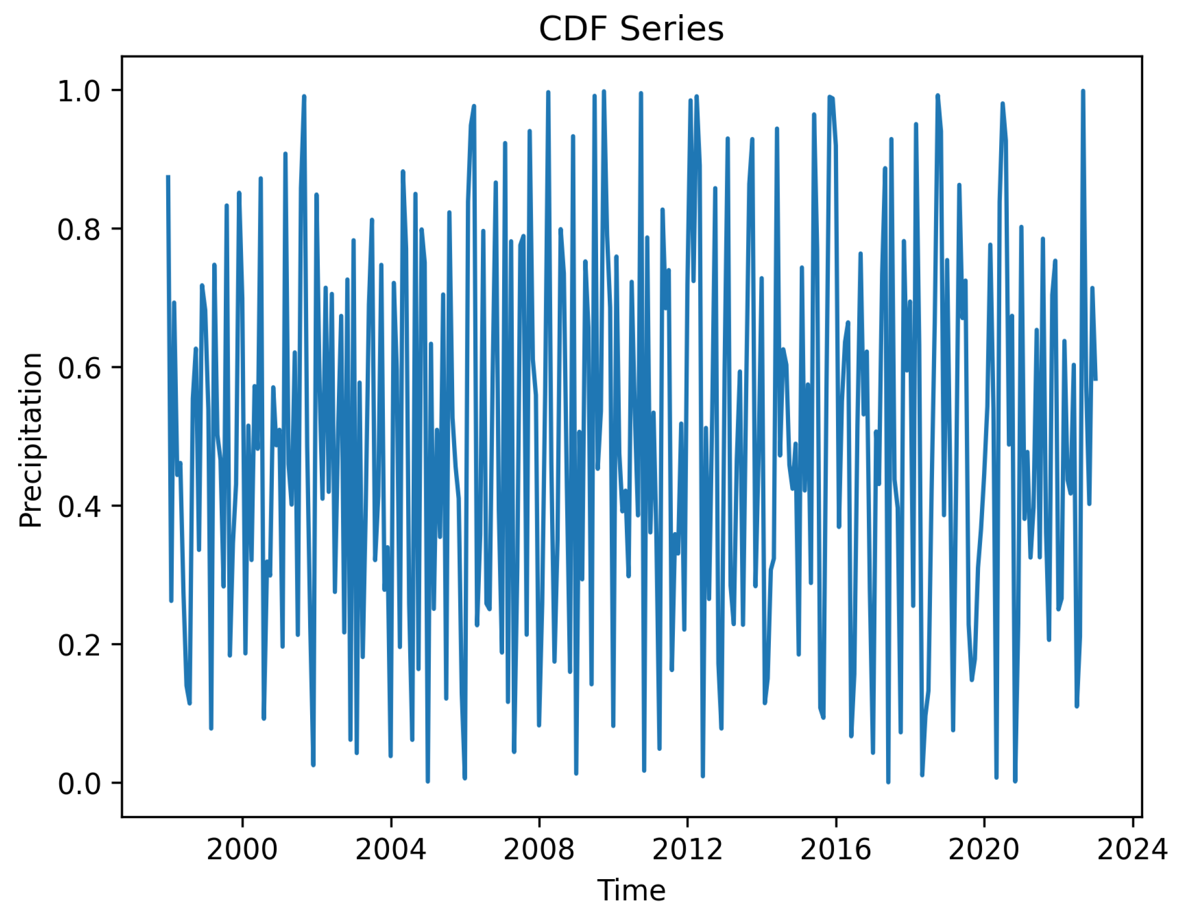
After estimating the GEV parameters (location, scale, and shape), the next step involves transforming the remainder series into its corresponding CDF values. This transformation serves to normalize the residuals into a bounded probability space [0, 1], which is especially useful for training neural networks in subsequent steps. Using the fitted GEV distribution, each data point in the remainder series is mapped to its CDF value, effectively representing the probability of observing a value less than or equal to that point under the fitted distribution. This probabilistic representation captures the extremeness of each observation in a consistent, scale-independent manner. The resulting CDF series retains the temporal structure of the original data while offering a more stable and interpretable input for modeling. As shown in Figure 6, the transformed series reflects the evolving distribution of normalized rainfall extremes over time, with values closer to 1 indicating more extreme events.

3.3. Model Forecasting Performance

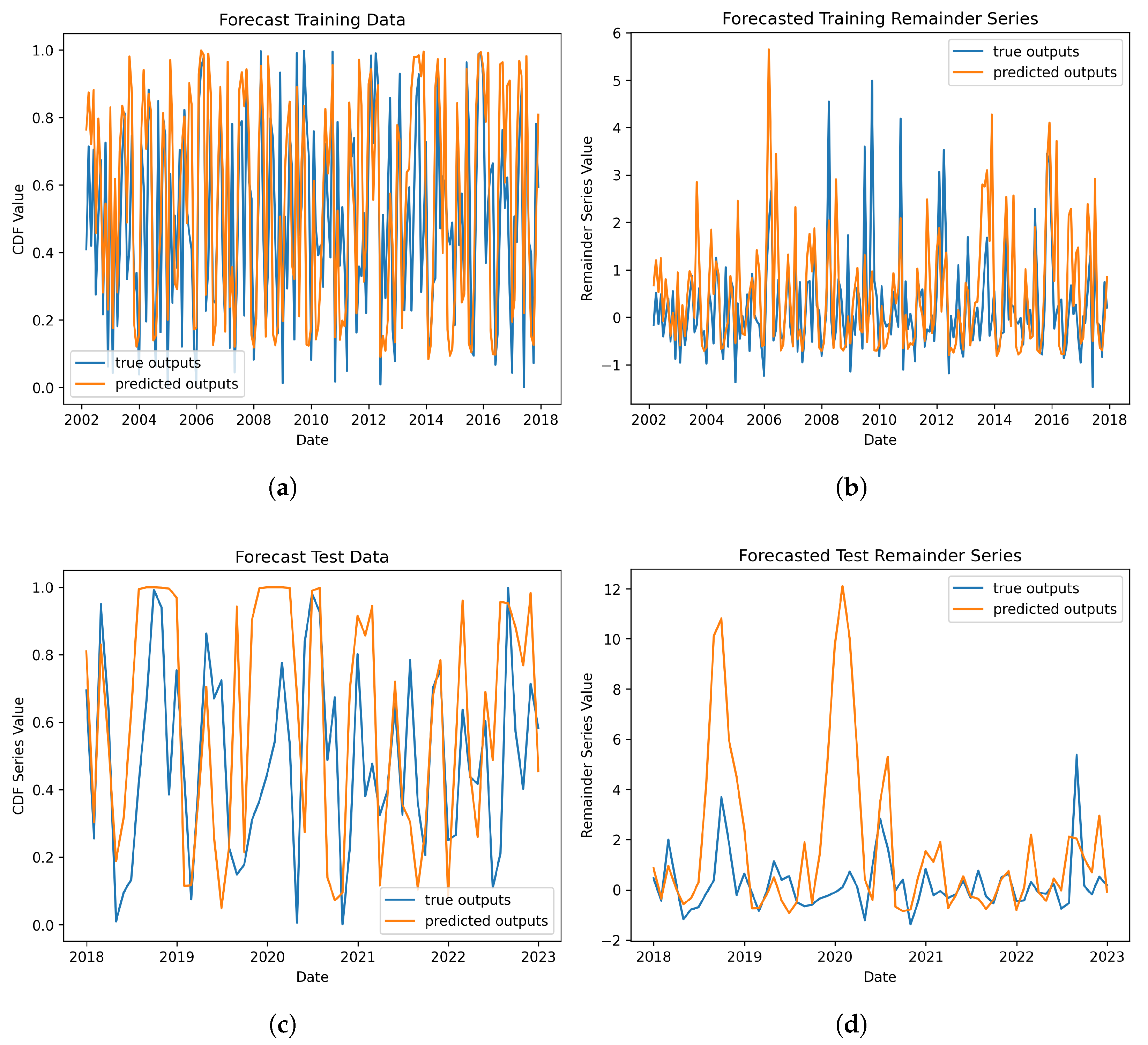
The four figures (Figure 7) collectively evaluate the performance of the LSTM trained to forecast precipitation extremes, specifically through the prediction of GEV-based CDF values and their inverse transformation to the original remainder scale. The first plot (Figure 7a) compares the predicted and true CDF outputs on the training dataset. The model captures the structure of the sequence well, maintaining consistency in the general amplitude and timing of fluctuations. Despite some local deviations, the predicted CDFs track the observed values closely, suggesting the model has effectively learned the temporal dependencies in the normalized space. The second plot (Figure 7b) shows the predicted versus true remainder values obtained by inverting the CDF forecasts. The predicted remainder series exhibits good alignment with the true series, especially in capturing the amplitude and occurrence of moderate-to-extreme values. This demonstrates that the model’s probabilistic learning in the CDF domain successfully transfers to accurate magnitude predictions in the original space. Similarly, Figure 7c,d display model performance on unseen test data. While more variability is observed, the model retains a reasonable ability to follow the general structure of the CDF sequence, including several sharp rises and falls associated with extreme events. This reflects moderate generalization capability. The model is able to detect the timing of some major peaks but occasionally overestimates the magnitude, particularly in the earlier part of the test period. This over-prediction of extreme values suggests that while the model is sensitive to tail behavior, an intended effect of the tail-weighted loss, it may benefit from further calibration to balance precision and magnitude accuracy in out-of-sample extremes.

This behavior can be attributed to several interacting factors. First, the inherent class imbalance in the training data, where extreme events are sparse compared to non-extreme observations, poses a significant challenge for deep learning models. While the tail-weighted loss helps the model focus on rare events, it may also amplify noise or overfit to a few extreme training points, especially if those points are not representative of the distribution seen in the test set. The result is a model that learns to “expect” more intense extremes than may actually occur in unseen data. Second, the use of a sigmoid activation function in the final output layer, while useful for bounding predictions between 0 and 1 in the CDF space, may introduce limitations when inverted back to the original remainder domain, particularly when the predicted CDF values are very close to 1. In such cases, small prediction errors can lead to disproportionately large remainder values after GEV inverse transformation, especially when the shape parameter is positive and the tail is heavy.

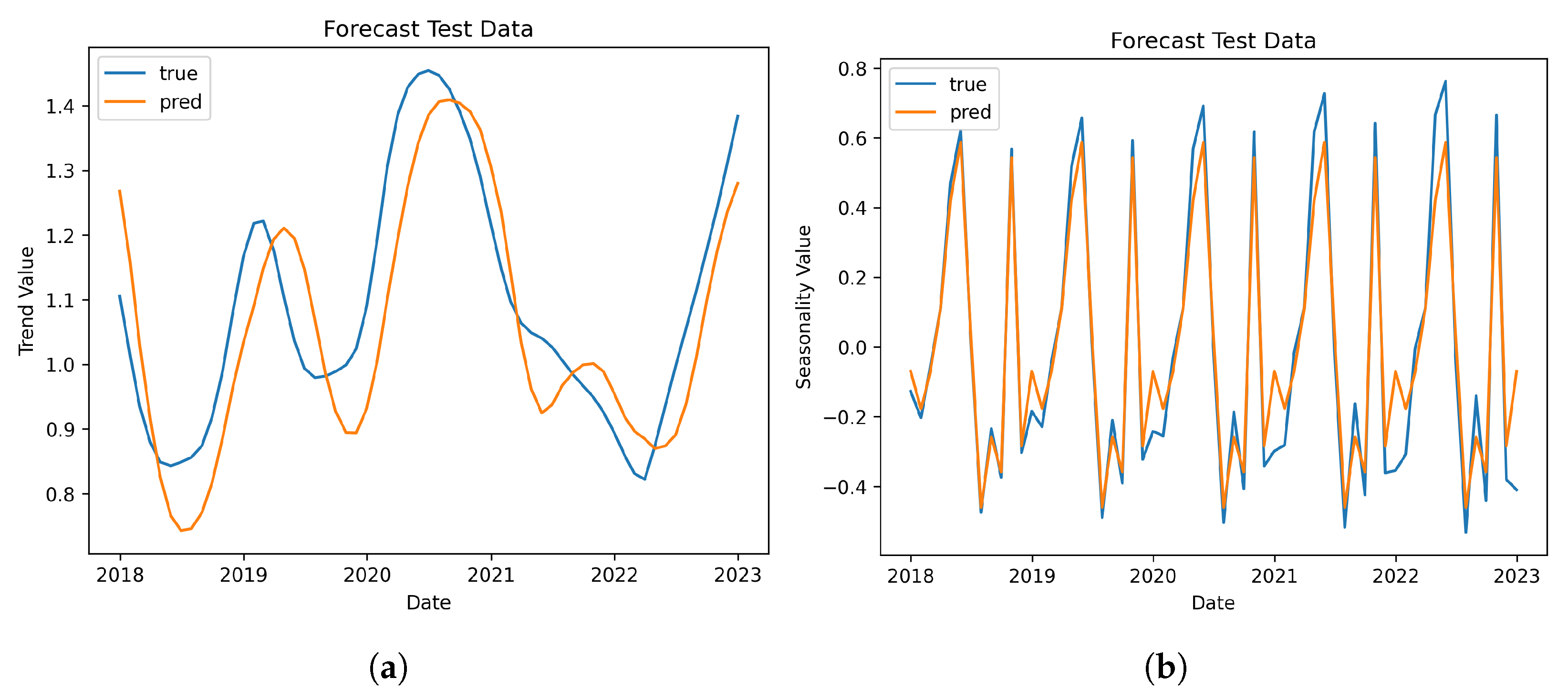
The performances of the trend and seasonality components on the test set were evaluated separately to assess the model’s ability to reconstruct the underlying structure of the precipitation series (Figure 8). For the trend component, a feedforward neural network was trained using a lag window of 50 months to predict smoothed, long-term variations. The model architecture consisted of multiple dense layers and was trained using MSE as the loss function. As shown in Figure 8a, the predicted trend closely follows the true trend curve over the test period, successfully capturing multi-year oscillations in baseline precipitation levels. While there are minor discrepancies in amplitude and timing, the model accurately reproduces the overall shape and turning points of the trend.

For the seasonal component, forecasting was achieved by recycling the last 12 months of the training seasonality series in a repeating cycle, under the assumption that seasonal patterns remain stable year to year. Figure 8b shows the predicted and true seasonality values over the test period. The repeated seasonal template aligns well with the actual seasonal signal, indicating that the periodic component of the precipitation series remained consistent and predictable across years. Together, these results demonstrate that the combined trend and seasonal reconstruction strategies provide a reliable foundation for interpreting and reconstructing the full precipitation time series, complementing the more complex modeling of the irregular remainder component.

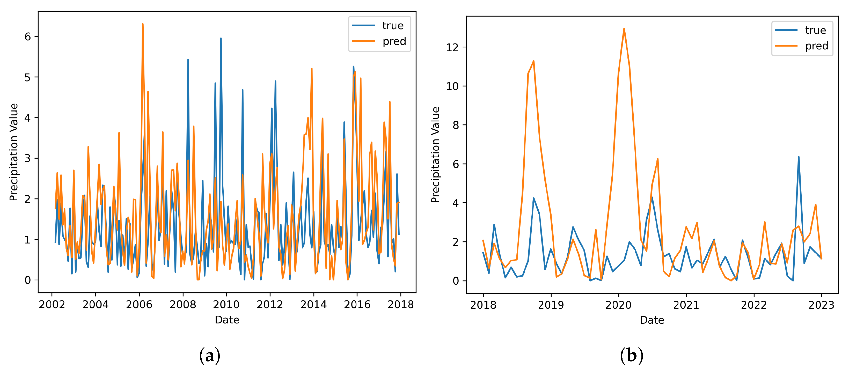
To obtain the final precipitation prediction, we add the outputs from the trend prediction, seasonality prediction, and remainder prediction models. The two figures (Figure 9) illustrate the final precipitation forecasts produced by the trained LSTM and deep forward neural networks, comparing predicted and observed monthly maximum precipitation values for both the training and test datasets. In the training dataset (Figure 9a), the model demonstrates strong agreement with the observed values, accurately capturing the magnitude, frequency, and timing of precipitation peaks across the historical period. This close alignment indicates that the model effectively learned the underlying relationships between input sequences and corresponding precipitation outcomes during training. In contrast, the test results (Figure 9b) show a more mixed performance. While the model still captures the timing of many extreme events, it tends to overestimate their magnitude, particularly during the years 2018 to 2020. This behavior reflects a tendency toward over-prediction in unseen data, a common challenge in tail-focused models trained on imbalanced extremes. Nevertheless, the model maintains reasonable alignment with the overall trend and frequency of events, suggesting its potential utility for identifying high-risk periods in a forecasting framework. Further calibration or post-processing could help temper the model’s overestimation of extreme values while preserving its sensitivity to peak events.

To evaluate the model’s ability to detect extreme precipitation events and assess its generalization capability, we conduct a POT analysis across all weather stations mentioned above. In this analysis, the 70th percentile of the true remainder series values is selected as the threshold for classifying extreme events. This choice effectively isolate the top 30% of precipitation anomalies, focusing the evaluation on the upper tail of the distribution where extreme events are most likely to occur. By applying this threshold, we exclude the bulk of moderate- or low-magnitude precipitation values and concentrate specifically on higher-impact events. This approach aligns with the goal of extreme value modeling, which prioritizes the accurate detection and characterization of rare, high-intensity occurrences rather than overall prediction performance across the entire dataset. This POT method provides a flexible, quantile-based evaluation of the model’s capability to recognize above-normal and potentially impactful rainfall extremes, making it particularly useful in hydrological forecasting and early warning applications. Binary labels are then created for both the ground truth and the model predictions, allowing the computation of standard classification metrics: precision, recall, and F1-score. Precision measures the proportion of predicted extreme events that are correct, while recall quantifies the proportion of actual extremes that the model successfully identifies. The F1-score represents the harmonic mean of precision and recall, offering a balanced metric of classification performance.

The model’s performance, as reported in

Table 1. The model performance on all weather stations. Figures of the training and testing performance are shared in Section 5.

Weather Station	POT (Inches/Hour)	Precision	Recall	F1-Score
RBD	1.48	0.48	0.84	0.62
ADS	0.64	0.57	0.33	0.42
DAL	1.66	0.44	0.29	0.35
LNC	1.63	0.30	0.21	0.25
DFW	1.73	0.75	0.25	0.38
GPM	0.78	0.42	0.53	0.47
GKY	1.50	0.75	0.67	0.71
HQZ	0.94	0.44	0.57	0.50
TKI	1.70	0.62	0.56	0.59
FTW	1.51	0.32	0.36	0.34
AFW	1.25	0.62	0.53	0.57
NFW	1.20	0.60	0.45	0.51
FWS	0.72	0.53	0.67	0.59
DTO	1.49	0.45	0.74	0.56
JWY	1.20	0.53	0.53	0.53
IAH	1.87	0.34	0.32	0.33
HOU	1.81	0.46	0.65	0.54
ELP	0.46	0.63	0.54	0.58

, shows noticeable variation in F1-scores across stations, driven not only by spatial heterogeneity but also by differences in data length and temporal variability. Stations such as GKY, RBD, and TKI achieved relatively high F1-scores (0.71, 0.62, and 0.59, respectively). These stations share a common data window from 2000 to 2020, a recent period characterized by more consistent instrumentation, fewer missing records, and relatively well-distributed extreme events—conditions that likely contributed to more effective model learning and generalization.

In contrast, stations such as DAL (F1 = 0.35) and DFW (F1 = 0.38) cover much longer historical periods (starting in 1946 and 1970, respectively). These extended time windows may introduce nonstationarities, such as changes in measurement practices, land use, or climate baselines, which can complicate model learning. Furthermore, LNC, while also spanning 2000–2020 like GKY and RBD, shows a remarkably flat remainder curve, suggesting limited variation in extreme precipitation signals. This lack of dynamic range likely contributed to its low F1-score of 0.25, as the model had little to learn from in terms of distinguishing extremes.

Overall, these results highlight the critical impact of the temporal window on model training and evaluation. Stations with consistent, high-resolution data over recent decades generally yield better performance, whereas longer or flatter records introduce challenges for capturing tail behaviors. This underlines the importance of accounting for temporal characteristics—such as variability, record length, and event richness—when designing and interpreting machine learning models for hydrological extremes.

4. Conclusions

This study proposes a novel end-to-end deep learning framework for forecasting monthly extreme precipitation by integrating statistical decomposition, extreme value theory, and tailored neural network learning. The key innovation lies in the combination of STL decomposition with Generalized Extreme Value (GEV)-based probabilistic transformation and a tail-weighted LSTM—specifically designed to improve sensitivity to rare but high-impact precipitation events. By decomposing the time series into trend, seasonality, and remainder components, the framework isolates the irregular (extreme) signal and applies a GEV distribution to transform the remainder into a bounded probabilistic space. A custom loss function, optimized through hyperparameter tuning, enables the LSTM to focus learning on tail events.

The final forecasts, produced by recombining the predicted components, demonstrate strong agreement with historical observations and effectively capture the timing of extreme events, even under data imbalance. To evaluate the model’s effectiveness in detecting extremes, a Peak Over Threshold (POT) analysis was performed across 18 weather stations using classification metrics such as precision, recall, and F1-score. Results show that the proposed method generalizes well across spatially diverse regions, with several stations achieving F1-scores above 0.55. While performance varied across sites, particularly in areas with fewer extreme events, the model consistently demonstrated its potential as a valuable tool for early warning systems and hydrological risk assessment. Overall, this work contributes a flexible, interpretable, and tail-aware deep learning approach for extreme precipitation forecasting.

Future work should focus on several key areas to enhance the model’s accuracy and applicability. These include integrating additional atmospheric and hydrological covariates to improve predictive power, exploring advanced model architectures such as attention mechanisms or transformer-based networks to better capture temporal dependencies, and developing data augmentation or resampling techniques to address class imbalance in extreme event detection. Furthermore, extending the model to real-time forecasting and assessing its performance under future climate scenarios could provide valuable insights for climate adaptation and disaster preparedness efforts.

5. Research Reproducibility

We acknowledge the importance of extending this work to other geographic regions and environmental settings, and we have identified this as a promising direction for future research. The current modeling framework is designed with flexibility in mind, allowing it to be adapted by researchers working in different local contexts. To facilitate this process, we have thoroughly documented our methodology and shared the source code, enabling others to replicate our results and tailor the approach to their own data. All results presented in this study are fully reproducible. The code and implementation details are publicly available on the author’s GitHub repository, https://github.com/hniu-tamu/Hydrology_extreme_precipitation_forecasting_with_LSTM, accessed on 27 July 2025.

References

1. Gleason, K.L.; Lawrimore, J.H.; Levinson, D.H.; Karl, T.R.; Karoly, D.J. A revised US climate extremes index. J. Clim. 2008, 21, 2124–2137. [Google Scholar] [CrossRef]
2. Kundzewicz, Z.W.; Kanae, S.; Seneviratne, S.I.; Handmer, J.; Nicholls, N.; Peduzzi, P.; Mechler, R.; Bouwer, L.M.; Arnell, N.; Mach, K.; et al. Flood risk and climate change: Global and regional perspectives. Hydrol. Sci. J. 2014, 59, 1–28. [Google Scholar] [CrossRef]
3. Kim, J.; Shu, E.; Lai, K.; Amodeo, M.; Porter, J.; Kearns, E. Assessment of the standard precipitation frequency estimates in the United States. J. Hydrol. Reg. Stud. 2022, 44, 101276. [Google Scholar] [CrossRef]
4. Tabari, H. Climate change impact on flood and extreme precipitation increases with water availability. Sci. Rep. 2020, 10, 13768. [Google Scholar] [CrossRef]
5. Wing, O.E.; Lehman, W.; Bates, P.D.; Sampson, C.C.; Quinn, N.; Smith, A.M.; Neal, J.C.; Porter, J.R.; Kousky, C. Inequitable patterns of US flood risk in the Anthropocene. Nat. Clim. Chang. 2022, 12, 156–162. [Google Scholar] [CrossRef]
6. Mishra, A.K.; Singh, V.P. Changes in extreme precipitation in Texas. J. Geophys. Res. Atmos. 2010, 115, D14106. [Google Scholar] [CrossRef]
7. Bhatia, N.; Singh, V.P.; Lee, K. Sensitivity of extreme precipitation in Texas to climatic cycles. Theor. Appl. Climatol. 2020, 140, 905–914. [Google Scholar] [CrossRef]
8. Gersonius, B.; Ashley, R.; Pathirana, A.; Zevenbergen, C. Climate change uncertainty: Building flexibility into water and flood risk infrastructure. Clim. Chang. 2013, 116, 411–423. [Google Scholar] [CrossRef]
9. Arnbjerg-Nielsen, K.; Fleischer, H. Feasible adaptation strategies for increased risk of flooding in cities due to climate change. Water Sci. Technol. 2009, 60, 273–281. [Google Scholar] [CrossRef]
10. Moore, T.L.; Gulliver, J.S.; Stack, L.; Simpson, M.H. Stormwater management and climate change: Vulnerability and capacity for adaptation in urban and suburban contexts. Clim. Chang. 2016, 138, 491–504. [Google Scholar] [CrossRef]
11. Heidari, B.; Prideaux, V.; Jack, K.; Jaber, F.H. A planning framework to mitigate localized urban stormwater inlet flooding using distributed Green Stormwater Infrastructure at an urban scale: Case study of Dallas, Texas. J. Hydrol. 2023, 621, 129538. [Google Scholar] [CrossRef]
12. Kourtis, I.M.; Tsihrintzis, V.A. Adaptation of urban drainage networks to climate change: A review. Sci. Total Environ. 2021, 771, 145431. [Google Scholar] [CrossRef]
13. Li, Y.; Xu, J.; Anastasiu, D.C. An extreme-adaptive time series prediction model based on probability-enhanced LSTM neural networks. In Proceedings of the AAAI Conference on Artificial Intelligence, Washington, DC, USA, 7–14 February 2023; Volume 37, pp. 8684–8691. [Google Scholar]
14. Sattari, A.; Foroumandi, E.; Gavahi, K.; Moradkhani, H. A probabilistic machine learning framework for daily extreme events forecasting. Expert Syst. Appl. 2025, 265, 126004. [Google Scholar] [CrossRef]
15. Najafi, M.S.; Kuchak, V.S. Ensemble-based monthly to seasonal precipitation forecasting for Iran using a regional weather model. Int. J. Climatol. 2024, 44, 4366–4387. [Google Scholar] [CrossRef]
16. Li, Y.; Lu, G.; Wu, Z.; He, H.; He, J. High-resolution dynamical downscaling of seasonal precipitation forecasts for the Hanjiang basin in China using the Weather Research and Forecasting Model. J. Appl. Meteorol. Climatol. 2017, 56, 1515–1536. [Google Scholar] [CrossRef]
17. Li, X.; Zhang, X.; Wang, S. A hybrid statistical downscaling framework based on nonstationary time series decomposition and machine learning. Earth Space Sci. 2022, 9, e2022EA002221. [Google Scholar] [CrossRef]
18. Sha, Y.; Sobash, R.A.; Gagne, D.J. Improving ensemble extreme precipitation forecasts using generative artificial intelligence. Artif. Intell. Earth Syst. 2025, 4, e240063. [Google Scholar] [CrossRef]
19. Tran Anh, D.; Van, S.P.; Dang, T.D.; Hoang, L.P. Downscaling rainfall using deep learning long short-term memory and feedforward neural network. Int. J. Climatol. 2019, 39, 4170–4188. [Google Scholar] [CrossRef]
20. Ng, K.; Huang, Y.; Koo, C.; Chong, K.; El-Shafie, A.; Ahmed, A.N. A review of hybrid deep learning applications for streamflow forecasting. J. Hydrol. 2023, 625, 130141. [Google Scholar] [CrossRef]
21. Ding, D.; Zhang, M.; Pan, X.; Yang, M.; He, X. Modeling extreme events in time series prediction. In Proceedings of the 25th ACM SIGKDD International Conference on Knowledge Discovery & Data Mining, Anchorage, AK, USA, 4–8 August 2019; pp. 1114–1122. [Google Scholar]
22. Sun, W.; Chen, H.; Guan, X.; Shen, X.; Ma, T.; He, Y.; Nie, J. Improved prediction of extreme rainfall using a machine learning approach. Adv. Atmos. Sci. 2025, 42, 1661–1674. [Google Scholar] [CrossRef]
23. Sønderby, C.K.; Espeholt, L.; Heek, J.; Dehghani, M.; Oliver, A.; Salimans, T.; Agrawal, S.; Hickey, J.; Kalchbrenner, N. Metnet: A neural weather model for precipitation forecasting. arXiv 2020, arXiv:2003.12140. [Google Scholar] [CrossRef]
24. Lin, K.C.; Chen, W.T.; Chang, P.L.; Ye, Z.Y.; Tsai, C.C. Enhancing the rainfall forecasting accuracy of ensemble numerical prediction systems via convolutional neural networks. Artif. Intell. Earth Syst. 2024, 3, 230105. [Google Scholar] [CrossRef]
25. Luo, G.; Cao, A.; Ma, X.; Hu, A.; Wang, C. Prediction of extreme precipitation events based on LSTM-self attention model. In Proceedings of the 2024 8th International Conference on Control Engineering and Artificial Intelligence, Shanghai, China, 26–28 January 2024; pp. 91–97. [Google Scholar]
26. Liu, X.; Zhao, N.; Guo, J.; Guo, B. Prediction of monthly precipitation over the Tibetan Plateau based on LSTM neural network. J. Geo-Inf. Sci. 2020, 22, 1617–1629. [Google Scholar]
27. Wang, W.C.; Ye, F.R.; Wang, Y.Y.; Gu, M. A singular spectrum analysis-enhanced BiTCN-selfattention model for runoff prediction. Earth Sci. Inform. 2025, 18, 31. [Google Scholar] [CrossRef]
28. Wang, C.H.; Yuan, J.; Zeng, Y.; Lin, S. A deep learning integrated framework for predicting stock index price and fluctuation via singular spectrum analysis and particle swarm optimization. Appl. Intell. 2024, 54, 1770–1797. [Google Scholar] [CrossRef]
29. Xiang, X.; Yuan, T.; Cao, G.; Zheng, Y. Short-term electric load forecasting based on signal decomposition and improved tcn algorithm. Energies 2024, 17, 1815. [Google Scholar] [CrossRef]
30. Iowa Environmental Mesonet. Iowa Mesonet: Iowa Environmental Mesonet (IEM) ASOS-AWOS-METAR Data, Iowa State University [data set]. Available online: https://www.mesonet.agron.iastate.edu/request/download.phtml?network=TX_ASOS (accessed on 13 October 2023).
31. RB, C. STL: A seasonal-trend decomposition procedure based on Loess. J. Off. Stat. 1990, 6, 3–73. [Google Scholar]
32. Dagum, E.B.; Bianconcini, S. Seasonal Adjustment Methods and Real Time Trend-Cycle Estimation; Springer: Berlin/Heidelberg, Germany, 2016; Volume 8. [Google Scholar]
33. Hyndman, R.J.; Athanasopoulos, G. Forecasting: Principles and Practice; OTexts: Melbourne, Australia, 2018. [Google Scholar]
34. Kennedy, J.; Eberhart, R. Particle swarm optimization. In Proceedings of the International Conference on Neural Networks, Perth, Australia, 27 November–1 December 1995; IEEE: New York, NY, USA, 1995; Volume 4, pp. 1942–1948. [Google Scholar]
35. Wang, D.; Tan, D.; Liu, L. Particle swarm optimization algorithm: An overview. Soft Comput. 2018, 22, 387–408. [Google Scholar] [CrossRef]
36. Solari, S.; Losada, M. A unified statistical model for hydrological variables including the selection of threshold for the peak over threshold method. Water Resour. Res. 2012, 48, W10541. [Google Scholar] [CrossRef]
Figure 1. Utilized ASOS stations (in red) of Texas. Multiple weather stations located in the Dallas–Fort Worth, Texas, area were selected. Additionally, two weather stations from the Houston, Texas, area (‘HOU’ and ‘IAH’) and one from El Paso, Texas (‘ELP’), were included.
Hydrology 12 00284 g001
Figure 2. A demonstration of the hourly precipitation dataset of RBD.
Hydrology 12 00284 g002
Figure 3. Monthly maximum precipitation at RBD weather station. Highest daily precipitation value within each month was selected to represent that month.
Hydrology 12 00284 g003
Figure 4. A demonstration of the STL decomposition at RBD weather station.
Hydrology 12 00284 g004
Figure 5. (a) Convergence plot of the GEV parameter estimation using the PSO method. The log-likelihood values steadily increase and stabilize within the first 60 iterations, indicating rapid and stable convergence of the optimization process. However, a total of 200 iterations is used to ensure general applicability across all weather stations, as some datasets may require a longer optimization horizon to achieve convergence. (b) Histogram of the STL remainder series with the fitted GEV probability density function. The histogram represents the empirical distribution of the remainder series from the training dataset.
Hydrology 12 00284 g005
Figure 6. Cumulative distribution function (CDF) series of the STL remainder component transformed using the fitted GEV distribution at RBD weather station.
Hydrology 12 00284 g006
Figure 7. Performance of the LSTM trained to forecast precipitation extremes, specifically through the prediction of GEV-based CDF values and their inverse transformation to the original remainder scale: (a) Forecasted CDF values on the training dataset. (b) Inverted remainder series predictions for the training dataset. (c) Forecasted CDF values on the test dataset. (d) Inverted remainder series predictions for the test dataset.
Hydrology 12 00284 g007
Figure 8. The forecasted trend and seasonality component on the test dataset: (a) Comparison of the predicted trend values generated by a feedforward neural network with the true STL-derived trend component over the test period. (b) The predicted seasonal pattern, constructed by cyclically repeating the last 12 months of training data, alongside the true STL-derived seasonality.
Hydrology 12 00284 g008
Figure 9. The final precipitation forecasts on the training and testing dataset: (a) This figure shows the predicted and true monthly maximum precipitation values over the training period. (b) This figure compares the predicted and observed monthly maximum precipitation values from 2018 to 2023. The LSTM captures the overall pattern and timing of many precipitation events, though it tends to overestimate the magnitude of certain extreme values.
Hydrology 12 00284 g009