Developing a Groundwater Quality Assessment in Mexico: A GWQI-Machine Learning Model

Abstract

Groundwater represents a critical global resource, increasingly threatened by overexploitation and pollution from contaminants such as arsenic (As), fluoride (F), nitrates (NO₃⁻), and heavy metals in arid to semi-arid regions like Mexico. Traditional Water Quality Indices ($WQIs$), while useful, suffer from subjectivity in assigning weights, which can lead to misinterpretations. This study addresses these limitations by developing a novel, objective Groundwater Quality Index ($GWQI$) through the seamless integration of Machine Learning (ML) models. Utilizing a database of 775 wells from the Mexican National Water Commission (CONAGUA), Principal Component Analysis (PCA) was applied to achieve significant dimensionality reduction. We successfully reduced the required monitoring parameters from 13 to only three key indicators: total dissolved solids (TDSs), chromium (Cr), and manganese (Mn). This reduction allows for an 87% decrease in the number of indicators, maximizing efficiency and generating potential savings in monitoring resources without compromising water quality prediction accuracy. Six $WQI$ methods and six ML models were evaluated for quality prediction. The Unified Water Quality Index (${WQI}_u$) demonstrated the best performance among the $WQIs$ evaluated and exhibited the highest correlation (R² = 0.85) with the traditional $WQI$ based on WHO criteria. Furthermore, the ML Support Vector Machine with polynomial kernel (svmPoly) model achieved the maximum predictive accuracy for ${WQI}_u$ (R² = 0.822). This robust $GWQI$-ML approach establishes an accurate, objective, and efficient tool for large-scale groundwater quality monitoring across Mexico, facilitating informed decision-making for sustainable water management and enhanced public health protection.

1. Introduction

Water plays an essential role in sustaining life and supporting numerous industrial transformation processes [1]. Within this framework, groundwater represents a critical source of freshwater for domestic, industrial, and agricultural purposes on a global scale [2]. In Mexico, reliance on groundwater is particularly significant, as it accounts for nearly 30% of the country’s total water use and supplies drinking water to approximately 40% of the population [2]. Nevertheless, the combined effects of overextraction and rising contamination are exerting unsustainable pressure on aquifers worldwide [2].

Mexico faces significant water security challenges. The arid and semi-arid regions of the north and central parts of the country, which cover over half of its territory, suffer from chronic water scarcity and are highly vulnerable to groundwater contamination [3]. Pollution sources may be both geogenic and anthropogenic in origin [2]. For examplecritical aquifers, such as those in the Comarca Lagunera, have been reported to contain elevated levels of arsenic (As), frequently surpassing the thresholds established by the World Health Organization (WHO) for safe human consumption [2,4,5]. The mobilization of As is intensified by severe overextraction of groundwater, particularly for agricultural irrigation, resulting in concentrations exceeding acceptable limits in over 90% of the region and exposing populations to As levels two to five times higher than those considered safe [2].

In addition to arsenic (As), groundwater in several regions of Mexico is affected by contamination from iron (Fe), fluoride (F), and manganese (Mn), elements that pose potential health risks due to chronic exposure through daily ingestion [4,6]. Nitrate (NO₃⁻), meanwhile, is considered the second most critical chemical contaminant in global groundwater resources. In Mexico, it is estimated that around 21 million individuals may be exposed to elevated nitrate concentrations, primarily resulting from intensive agricultural practices and discharges from urban areas [7]. Furthermore, the presence of emerging organic contaminants (EOCs) and endocrine-disrupting compounds (EDCs) represents an increasing environmental and public health concern, particularly in regions where untreated wastewater is used for agricultural irrigation, facilitating the infiltration of these pollutants into shallow aquifers [8]. Excessive groundwater withdrawal also contributes to land subsidence and the deterioration of water quality [9].

Given the multifaceted nature of water quality challenges, the use of robust assessment tools becomes indispensable. Water quality indexes ($WQIs$), which consolidate multiple physicochemical parameters into a single, interpretable value, serve as practical instruments for conveying essential information to policymakers and resource managers [10,11]. Despite their utility, conventional $WQI$ methodologies may present limitations. In particular, their application in arid and semi-arid regions can lead to misleading classifications—labeling water as safe for human consumption even when concentrations of specific contaminants exceed regulatory thresholds [4]. Therefore, the selection and implementation of $WQI$ models must be tailored to the local environmental context, considering the variability of influencing factors and the inherent heterogeneity of water quality [4].

Various investigations have been carried out in Mexico with the aim to develop groundwater quality indexes ($GWQIs$) tailored to local conditions. In the Comarca Lagunera region, one such study assessed groundwater quality and formulated a specific $GWQI$ designed for evaluating suitability for human consumption. This was in response to the inadequacy of conventional indices in areas with elevated contamination levels. For instance, although the previously used weighted arithmetic water quality index ($WAWQI$) classified groundwater samples as being in “excellent” or “good” condition, 95% of these samples surpassed the regulatory limits for As, 33% for fluoride (F), and 11% for uranium (U) [4]. This mismatch resulted in a misleading perception of water safety. Conversely, the newly developed index revealed that only two of the samples could be accurately classified as “excellent” and suitable for consumption without the need for pretreatment.

In northeastern Mexico, a study conducted in the El Potosí, Sandia, and Cieneguilla watersheds evaluated groundwater quality for both drinking and irrigation purposes using $WQI$ methodologies [12]. The analysis indicated that between 69% and 93% of the samples were classified as having “excellent” or “good” quality for human consumption. Nevertheless, salinity levels in 7% to 31% of the samples exceeded the thresholds established by the World Health Organization (WHO). In the El Potosí watershed, 13% of the samples contained fluoride (F) concentrations above 1.5 mg L⁻¹, levels associated with the risk of dental and skeletal fluorosis [13]. In the Sandia watershed, 13% of the samples exhibited elevated NO₃⁻ concentrations above 42 mg L⁻¹, likely resulting from the application of synthetic fertilizers, posing a potential health risk.

In south central Mexico, an assessment was conducted on the water quality of Lake Coatetelco and surrounding groundwater wells to determine their suitability for drinking and irrigation, as well as to evaluate potential health risks associated with NO₃⁻ and F exposure. Although the majority of samples collected following the warm rainy season were rated as “excellent” or “good” based on the drinking water quality index ($DWQI$ < 100), 50% exceeded the F threshold of 1.5 mg L⁻¹. The total hazard quotient index ($THQI$) revealed at least one lake sample and 53% of the groundwater samples may present F related health risks for both adults and children. Conversely, NO₃⁻ concentrations remained within the limits established by the WHO [5]. These findings underscore the complexity of groundwater quality assessment in Mexico and emphasize the importance of expanding the geographical coverage of studies, promoting interdisciplinary collaboration, and developing more precise monitoring tools to ensure sustainable water management and enhanced public health protection.

To address the limitations of conventional methodologies and enhance the precision and adaptability of groundwater quality assessments, machine learning (ML) has emerged as a highly promising approach. ML algorithms have shown notable effectiveness and practicality in modeling and predicting various aspects of water resources, including water quality, due to their capacity to simultaneously process heterogeneous datasets and operate with lower computational and financial costs than traditional models [4,14]. Nevertheless, despite the critical challenges posed by groundwater depletion and contamination in Mexico, the application of ML techniques for forecasting groundwater levels and assessing water quality remains largely underutilized in the region [14].

This research aims to develop an integrated model for groundwater quality assessment in Mexico by combining the conceptual framework of $WQIs$ with the analytical strength of ML models to construct and optimize a novel $GWQI$. The primary goal is to create a robust, context-specific tool tailored to the country’s unique hydrogeological and contamination scenarios, thereby enhancing decision-making processes for the sustainable management of groundwater and the safeguarding of public health. The central hypothesis posits that PCA will effectively identify the most significant indicators of groundwater quality. The integration of these indicators into various $WQI$ methodologies and ML models are expected to enable a more objective, efficient, and accurate evaluation and prediction of groundwater quality in the Mexican context.

2. Materials and Methods

2.1. Study Area

Mexico, located in the southern region of North America, extends latitudinally from 14°32′27″ to 32°43′06″ north and longitudinally from 86°42′36″ to 118°27′24″ west, covering an area of approximately 1.96 million km² [15]. Intense tectonic activity during the Cenozoic era has resulted in Mexico’s complex orography, creating a diverse landscape that ranges from coastal lowlands to high elevations, such as the Pico de Orizaba [15]. The territory is marked by important mountain systems such as the Sierra Madre Oriental, Sierra Madre Occidental, and the Trans-Mexican Volcanic Axis, which contribute to its varied topography [15]. Additionally, flat, elongated valleys oriented from northwest to southeast, separated by high, narrow mountain ranges, characteristic of the physiographic provinces of mountains and basins [1].

The nation’s geography and topography significantly influence its weather patterns. Although 66% of Mexico experiences arid or semi-arid conditions, receiving less than 500 mm of annual rainfall, whereas the southeastern region is considerably wetter, with precipitation ranging from 800 to 5000 mm per year [3,15]. On average, precipitation in Mexico is approximately 740 mm per year, with an average temperature of 14.7 °C [15]. Precipitation (Rainfall) primarily occurs during the summer months (June and September), often in the form of heavy downpours [3,15]. The warmest months are recorded between April and May, with average temperatures close to 25 °C. The arid regions of northern and central Mexico are particularly vulnerable to the impacts of climate change, with projected intensification of droughts and greater variability in precipitation patterns, affecting water availability and quality [3]. Figure 1 shows the geographic location of Mexico and its different regions.

2.2. Database

The database used was developed by the National Water Commission of Mexico (CONAGUA, Spanish acronym), the agency in charge of monitoring and controlling surface and groundwater in the country. The database used focuses on monitoring the groundwater conditions of 775 wells nationwide for the year 2022 (https://sigagis.conagua.gob.mx/gas1/index.html, accessed on 27 September 2025), to which 13 quality-related indicators are determined, as shown in

Table 1. Indicators analyzed for groundwater.

Indicator	Levels	Criteria	Indicator	Levels	Criteria
ALK	$ALK<20$	Undesirable	FLU	$FLUO>5000$	High
	$20\le ALK<75$	Low		$0.7\le FLUO<1.5$	Optimum
	$75\le ALK\le 150$	Medium		$0.4\le FLUO<0.7$	Medium
	$ALK>150$	Undesirable		$0.0\le FLUO<0.4$	Low
EC	$EC\le 250$	Excellent for irrigation	TDS	$TDS\le 500$	Excellent for irrigation
	$250<EC\le 750$	Good for irrigation		$500<TDS\le 1000$	Use for sensitive crops
	$750<EC\le 2000$	Permissible for irrigation		$1000<TDS\le 2000$	Use for special handling crops
	$2000<EC\le 3000$	Doubtful for irrigation		$2000<TDS\le 5000$	Use for tolerant crops
	$EC>3000$	Undesirable for irrigation		$TDS>5000$	Undesirable for irrigation
FCL	$FCL<1.1$	Excellent	HRD	$HRD\le 60$	Mild
	$1.1\le FCL\le 200$	Good		$60<HRD\le 120$	Moderately mild
	$200<FCL\le 1000$	Acceptable		$120<HRD\le 500$	Hard
	$1000<FCL\le \mathrm{10,000}$	Polluted		$HRD>500$	Very hard
	$FCL>\mathrm{10,000}$	Heavily polluted
NO3−	$N{O}_3\le 5$	Excellent	As	$As\le 0.01$	Excellent
	$5<N{O}_3\le 11$	Good		$0.01<As\le 0.025$	Suitable
	$N{O}_3>11$	Unsuitable		$As>0.025$	Unsuitable
Cd	$Cd\le 0.003$	Excellent	Mn	$Mn\le 0.15$	Excellent
	$0.003<Cd<\le 0.005$	Suitable		$0.15<Mn\le 0.40$	No health effect
	$Cd>0.005$	Unsuitable		$Mn>0.40$	No health effect
Hg	$Hg\le 0.006$	Excellent	Pb	$Pb\le 0.01$	Excellent
	$Hg>0.006$	Unsuitable		$Pb>0.01$	Unsuitable
Fe	$Fe\le 0.3$	Excellent	Cr	$Cr\le 0.05$	Excellent
	$Fe>0.3$	No health effect		$Cr>0.05$	Unsuitable

ALK, alkalinity (mg L⁻¹); FLU, fluorides (mg L⁻¹); EC, electrical conductivity (µS cm⁻¹); TDS, total dissolved solids (mg L⁻¹); FCL, fecal coliforms (MPN 100 mL⁻¹); HRD, hardness (mg L⁻¹); NO₃⁻, nitrates (mg L⁻¹); As, arsenic (mg L⁻¹); Cd, cadmium (mg L⁻¹); Mn, manganese (mg L⁻¹); Hg, mercury (mg L⁻¹); Pb, lead (mg L⁻¹); Fe, iron (mg L⁻¹); Cr, chromium (mg L⁻¹).

.

2.3. Data Processing

Data processing is an essential step in implementation of regression models in ML. In the present database, the treatment consisted of the imputation by arithmetic mean of the missing data, as well as the correction of outliers by imputation by capping at the P5 and P95 percentiles. In addition, prior to implementation in the regression models, the data distribution was normalized by means of the Box–Cox transformation technique, as well as standardization of the data by means of the minmax function [15,16,17].

2.4. PCA

In order to reduce the dimensionality of the database and select those indicators with the most significant relationship with water quality, a PCA was performed, starting with a Kaiser-Meyer-Olkin fit analysis [16,18]. Principal components (PCs) were chosen based on the eigenvalue criterion (eigenvalue ≥ 1) [19]. Once PCs were established, a Spearman correlation matrix was performed, followed by a redundancy reduction process, with the aim of eliminating those indicators related to each other [20]. The indicators resulting from the process were used for the prediction of the quality values of the various established indexes [21,22].

2.5. Water Quality Indexes Used (WQI)

2.5.1. WQI

The $WQI$ is a technique that enables the integration of water quality indicators into a single standard value that allows comparison between different water bodies. This index is widely used worldwide and will be used as a reference for comparing the new indexes developed in this study. The process for implementing the $WQI$ is divided into five stages, the first being the assignment of weights $\left(w_i\right)$ to the indicators analyzed, in accordance with WHO guidelines and Mexican legislation [23], which for the present study are located in

Table 2. Standard values and weights of indicators analyzed [6,25,26].

Inticators	Standard Values	${\mathit{w}}_{\mathit{i}}$	Inticators	Standard Values	${\mathit{w}}_{\mathit{i}}$
ALK	400	5	FLU	1.5	4
EC	1500	2	TDS	1000	2
FCL	1000	4	HRD	100	2
NO3−	50	5	As	0.01	5
Cd	0.003	5	Mn	0.1	2
Hg	0.006	5	Pb	0.01	5
Fe	0.3	2	Cr	0.05	5

$w_i$, indicator weight; ALK, alkalinity (mg L⁻¹); FLU, fluorides (mg L⁻¹); EC, electrical conductivity (µS cm⁻¹); TDS, total dissolved solids (mg L⁻¹); FCL, fecal coliforms (MPN 100 mL⁻¹); HRD, hardness (mg L⁻¹); NO₃⁻, nitrates (mg L⁻¹); As, arsenic (mg L⁻¹); Cd, cadmium (mg L⁻¹); Mn, manganese (mg L⁻¹); Hg, mercury (mg L⁻¹); Pb, lead (mg L⁻¹); Fe, iron (mg L⁻¹); Cr, chromium (mg L⁻¹).

[24]:

The second stage consists of calculating the relative weight of each of the indicators analyzed using Equation (1).

$$W_i={\displaystyle \frac{w_i}{{\sum }_{i=1}^n{w}_i}}$$

(1)

where $n$ is the number of indicators analyzed, $w_i$ refers to the weight established by the WHO for each of the indicators analyzed, while $W_i$ is the relative weight for each of the indicators analyzed.

The third stage consists of calculating the quality rating scale for each indicator analyzed, which is established from Equation (2).

$$q_i={\displaystyle \frac{C_i}{S_i}}\times 100$$

(2)

where $q_i$ is the quality scale, $C_i$ refers to the concentration of each of the indicators analyzed and $S_i$ are the standard values of the indicators analyzed established by the WHO.

The fourth stage refers to the calculation of the water quality sub-index, which is obtained with Equation (3).

$${SI}_i=W_i\times q_i$$

(3)

where ${SI}_i$ refers to the water quality sub-index.

The final stage is the calculation of the $WQI$, which is performed from Equation (4).

$$WQI=\sum {SI}_i$$

(4)

The $WQI$ divides water quality based on its values into five categories, which are shown in

Table 3. Quality levels of the $WQI$.

Level	Quality
$WQI<50$	Excellent
$50\le WQI<100$	Good
$100\le WQI<200$	Poor
$200\le WQI<300$	Very poor
$WQI\ge 300$	Unsuitable for drinking

$WQI$, water quality index.

.

2.5.2. Entropy Weighted Water Quality Index ($EWQI$)

The $EWQI$ is developed with the purpose to reduce errors introduced by the subjective expert assignment of weights for the analyzed indicators. The calculation of this index is performed as follows, starting with the creation of a performance matrix, where each monitored indicator of each of the wells is entered [11,27].

$$X=\left[\begin{array}{cc}{x}_{11}& x_{12}\\ x_{21}& x_{22}\\ x_{m1}& x_{m2}\end{array}\dots \begin{array}{c}{x}_{1n}\\ x_{2n}\\ x_{mn}\end{array}\right]$$

(5)

where $X$ represents the matrix, $m$ refers to each of the indicators analyzed and $n$ refers to each of the wells analyzed.

Subsequently, a normalization of the matrix is performed, which allows comparing the different indicators analyzed regardless of the units. This is done from Equation (6).

$$v_{ij}={\displaystyle \frac{x_{ij}}{{\sum }_{i=1}^m{x}_{ij}}}$$

(6)

where $v_{ij}$ refers to the normalized matrix, $x_{ij}$ refers to each one of the arrays of each column.

Once that is done, we proceed to the entropy calculation for each of the indicators analyzed, using Equation (7).

$$z_j={\displaystyle \frac{1}{ln\left(m\right)}}{\sum }_{i=1}^m{v}_{ij}ln\left(v_{ij}\right)$$

(7)

where $z_j$ refers to the entropy value of each indicator analyzed.

Once this has been done, we proceed with the calculation of the objective weights of each of the indicators analyzed, based on Equation (8).

$$W_j={\displaystyle \frac{1-z_j}{{\sum }_{i=1}^{n}1-z_j}}$$

(8)

where $W_j$ refers to the target weight of each of the indicators.

At the same time, the scale factor is also calculated, based on Equation (9).

$$q_j=\left[{\displaystyle \frac{V_j-V_{id}}{S_j-V_{id}}}\right]\times 100$$

(9)

where $q_j$ is the quality factor of each of the analyzed indicators, $V_j$ is the measured value for each of the indicators, $S_j$ is the standard allowed value of each of the analyzed indicators assigned by WHO [26], and $V_{id}$ is the ideal value of each of the analyzed indicators in pure water.

To conclude, the $EWQI$ can be calculated from Equation (10).

$$EWQI=\sum _{i=1}^n{W}_j\times q_j$$

(10)

The $EWQI$ presents water quality results grouped into five categories, which are presented in Table 3.

2.5.3. Water Quality Index Unified (${WQI}_u$)

Like the $EWQI$, the ${WQI}_u$ was developed to reduce the errors introduced by the subjective expert assignment of the weights of the indicators analyzed, which is proposed in this research. The weights of the indicators analyzed were established from the proportion of variability of the PCs resulting from the PCA, which are shown in

Table 4. Weights of analyzed parameters of the ${WQI}_u$.

Indicators	${\mathit{w}}_{\mathit{u}\mathit{i}}$	Indicators	${\mathit{w}}_{\mathit{u}\mathit{i}}$
ALK	0.235	FLU	0.112
EC	0.235	TDS	0.235
FCL	0.235	HRD	0.235
NO3−	0.235	As	0.112
Cd	0.072	Mn	0.103
Hg	0.189	Pb	0.189
Fe	0.189	Cr	0.072

$w_{ui}$, unified weight of indicators analyzed; ALK, alkalinity; FLU, fluorides; EC, electrical conductivity; TDS, total dissolved solids; FCL, fecal coliforms; HRD, hardness; NO₃⁻, nitrates; As, arsenic; Cd, cadmium; Mn, manganese; Hg, mercury; Pb, lead; Fe, iron; Cr, chromium.

.

The ${WQI}_u$ presents water quality results grouped into five categories, which are presented in Table 3.

2.5.4. Heavy Metal Evaluation Index ($HEI$)

This $HEI$ provides an overview of water quality with respect to heavy metal concentrations. This index is calculated from the maximum allowable concentrations of the heavy metals analyzed, as shown in Equation (11) [11].

$$HEI={\sum }_{i=1}^n{HEI}^i$$

(11)

where $n$ is the number of analyzed heavy metals, ${HEI}^i$ is the contamination index corresponding to each of the heavy metals, which is calculated from Equation (12).

$${HEI}^i={\displaystyle \frac{M_i}{H_{mac}^i}}$$

(12)

where $H_{mac}^i$ is the maximum allowable concentration of the analyzed heavy metal, $M_i$ refers to the current measured concentration of the analyzed metal. The possible results of this index allow dividing water quality into three categories based on the degree of contamination, as shown in

Table 5. Quality levels of the $HEI$.

Level	Contamination
$HEI<10$	Low
$10\le HEI\le 20$	Moderate
$HEI>20$	High

$HEI$, heavy metal evaluation index.

.

2.5.5. Nemerow Index ($NeI$)

This index is multifactorial integrated; it establishes the concentrations of heavy metals analyzed from Equation (13) [11].

$$NeI=\sqrt{{\displaystyle \frac{{\left(M_i/I_i\right)}_{mean}^2+{\left(M_i/I_i\right)}_{max}^2}{n}}}$$

(13)

where $I_i$ is the maximum allowable concentration of the heavy metal analyzed.

This index classifies water quality into four categories, as shown in

Table 6. Quality levels of $NeI$.

Level	Contamination
$NeI<1$	Negligible
$1\le NeI<2.5$	Slight
$2.5\le NeI<7$	Moderate
$NeI\ge 7$	Contaminated

$NeI$, nemoro index.

.

2.5.6. Ecological Risks of Heavy Metals in Groundwater ($ERI$)

This index is used to evaluate the potential risk associated with the concentration of heavy metals in the groundwater, which is calculated from Equation (14) [11].

$$ERI={\sum }_{i=1}^n\left[T_i\times \left(M_i/I_i\right)\right]$$

(14)

where $T_i$ refers to the biological toxicity factor of each of the heavy metals analyzed, which are established in

Table 7. Factors of biological toxicity of heavy metals [25,28,29].

Heavy Metal	${\mathit{T}}_{\mathit{i}}$
As	10
Cd	30
Cr	2
Hg	40
Pb	5
Mn	1
Fe	1

$T_i$, toxicity factor; As, arsenic; Cd, cadmium; Cr, chromium; Hg, mercury; Pb, lead; Mn, manganese; Fe, iron.

.

This index establishes groundwater quality in four categories, as shown in

Table 8. Quality levels of the $ERI$.

Level	Risk
$ERI<110$	Low
$110\le ERI<200$	Moderate
$200\le ERI<400$	Considerable
$ERI\ge 400$	Very High

$ERI$, ecological risks of heavy metals.

.

2.6. Index Performance Evaluation

To evaluate the performance of the different indexes established, their analysis was carried out through the establishment of two different indexes, the first, a sensitivity index ($SI$) (Equation (15)), which analyzes the variability of the quality results obtained by the different indexes, and an efficiency rate index ($ER$), which analyzes the precision of the quality results obtained with the different indexes and its correlation with the 13 indicators analyzed (Equation (16)).

$$SI={\displaystyle \frac{X_{max}}{X_{min}}}$$

(15)

$$\mathrm{E}\mathrm{R}={\displaystyle \frac{K}{N}}\times 100$$

(16)

where $X_{max}$ and $X_{min}$ refers to the maximum and minimum quality value obtained by each of the quality indexes respectively, $K$ is the number of significant correlations between the different quality indexes and the indicators analyzed, and $N$ is the number of indicators analyzed.

2.7. ML Models Developed

In the present study, six ML models were established for the prediction of the quality values of the six established $WQIs$, which were boosted generalized additive model (gamboost), support vector machines with polynomial kernel (svmPoly), decision trees and multiple linear regression methods (cubist), random forest (rf), neural network (nnet) and robust linear model (rlm) [16,30]. All the statistical analyses were conducted using software R version 4.3.0 [31], using the caret package [21,32]. For the establishment of the models, the database was separated into two, the first one with 80% of the observations (620 elements) was established as the training database, the second one, with the remaining 20% of the observations (155 elements) was established as the test database, to validate the prediction efficiency of the developed ML models [16].

The establishment of ML models and their hyper-parameters whose number depends on the type of model, are an essential step in the implementation of any modeling. A random search grid adaptive resampling was performed for the optimal establishment of the hyper-parameters of each model [16,33]. One thousand variations of each of the established models were generated, selecting those hyper-parameters that presented lower values of the evaluation criteria of Section 2.8. The models developed and the values of the hyper-parameters established are presented in

Table 9. ML models established [32].

Model		Hyper-Parameters
gamboost	mstop = 112	pruene = no	---
cubist	committees = 44	neighbors = 0	---
nnet	size = 5	decay = 0.0007243555	---
rf	mtry = 2	---	---
rlm	intercept = True	psi = psi.bisquare	---
svmPoly	degree = 2	scale = 0.05776932	C = 731.8544

Gamboost, generalized additive boosted additive model; cubist, decision trees and multiple linear regression methods; rf, random forest; nnet, neural network; rlm, robust linear model; svmPoly, support vector machines with polynomial kernel; mstop, number of boosting iterations (numeric); prune, AIC pruning (character); committees, number of committees (numeric); neighbors, number of instances (numeric); size, number of hidden units (numeric); decay, weight decay (numeric); mtry, number of randomly selected predictors (numeric); intercept, intercept (numeric); psi, psi (character); degree, polynomial degree (numeric); scale, scale (numeric); C, cost (numeric).

below.

2.8. Model Evaluation Criteria

To compare the different ML models developed and their efficiency in predicting water quality values, the following criteria will be used.

2.8.1. Mean Absolute Error ($MAE$)

This criterion gives an estimate of the absolute differences between the predicted and observed values for each of the wells analyzed and is defined from Equation (17) [24,34].

$$MAE={\displaystyle \frac{1}{N}}{\sum }_{i=1}^N\left|{\widehat{X}}_i-X_i\right|$$

(17)

It is considered a better model when MAE has values close to zero.

2.8.2. Root Mean Squared Error ($RMSE$)

It refers to the root of the deviation between the observed values and those predicted by the model, calculated from Equation (18) [24,34].

$$RMSE=\sqrt{{\displaystyle \frac{1}{N}}{\sum }_{i=1}^N{\left({\widehat{X}}_i-X_i\right)}^2}$$

(18)

where for both $MAE$ and $RMSE$, ${\widehat{X}}_i$ is the value predicted by the model, $X_i$ is the observed value and $N$ is the number of observations made.

It is considered as a better model when $RMSE$ presents values close to zero [24,34].

2.8.3. Corrected Akaike Information Criterion ($AICc$)

It is a standard selection criterion for models, it makes a trade-off between model complexity and model accuracy, and is established from Equation (19) [35].

$$AICc=Nlog\left(L\right)+2K\left({\displaystyle \frac{N}{N-K-1}}\right)$$

(19)

It is considered a better model when $AICc$ has lower values.

2.8.4. Bayesian Information Criterion ($BIC$)

It is an asymptotic approximation of the Bayesian posterior transformation of the probability of a model, which is computed from Equation (20) [24,34].

$$BIC=Nln\left(L\right)+Kln\left(N\right)$$

(20)

where for both $AICc$ and $BIC$, $N$ is the number of observations, $L$ is the likelihood function, $K$ is the number of indicators analyzed. It is considered better when $AICc$ and $BIC$ present low values.

2.8.5. Coefficient of Determination (R²)

It can be interpreted as the proportion of variance of the independent variable that is subject to being predicted by independent predictor variables, and can be calculated from Equation (21) [24,34].

$$R^2=1-{\displaystyle \frac{{\sum }_{i=1}^N{\left(X_i-{\widehat{X}}_i\right)}^2}{{\sum }_{i=1}^N{\left(X_i-{\overline{X}}_i\right)}^2}}$$

(21)

where ${\overline{X}}_i$ is the average value of the measurements of the indicators analyzed. The best model is considered to be the one with values close to one.

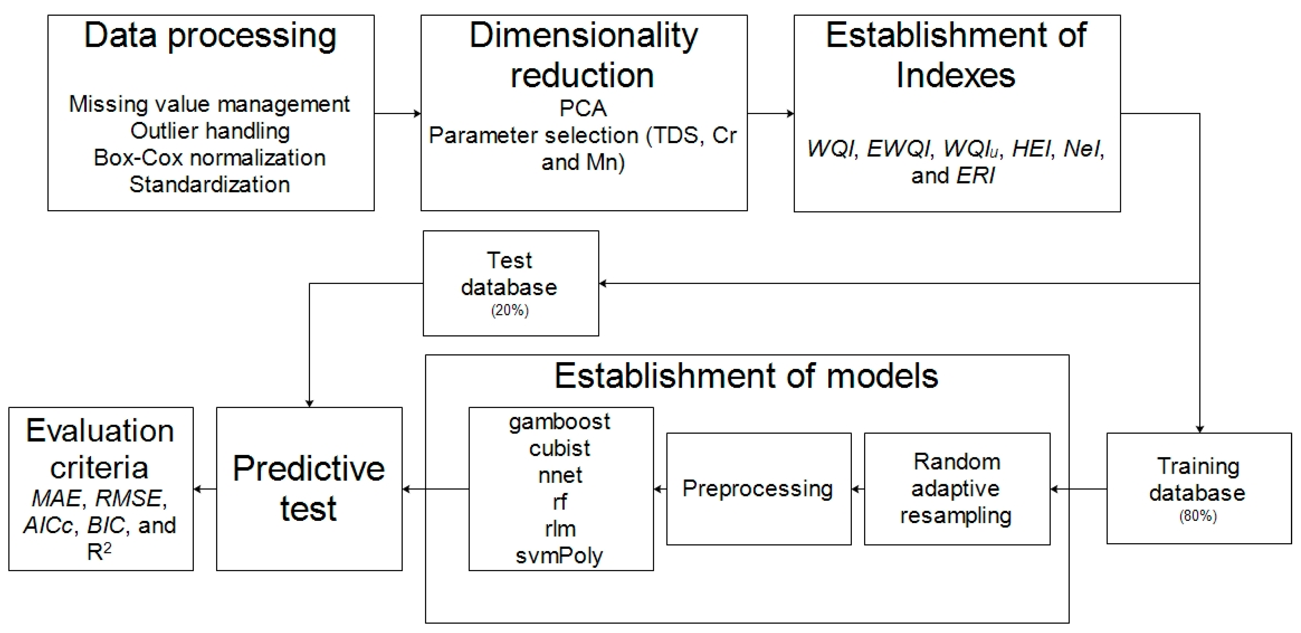
In order to provide the reader with a clearer understanding of the research workflow, Figure 2 is shown below.

3. Results and Discussion

3.1. Descriptive Statistics

Table 10. Descriptive statistics of indicators analyzed.

Indicators	Mean, n = 775	Min	1st Q	Median	3rd Q	Max	p
FCL	402.5 (765)	1.1	1.1	1.1	120.0	1928.6	<0.001
EC	1128.1 (794)	103.0	525.5	932.0	1467.5	3086.2	<0.001
TDS	875.0 (577)	120.0	443.0	753.0	1005.0	2300.0	<0.001
FLU	0.781 (0.71)	0.200	0.295	0.530	0.944	2.833	<0.001
HRD	374.3 (252)	10.0	186.5	354.0	451.6	1016.2	<0.001
ALK	237.2 (86)	50.8	177.6	244.4	286.3	442.7	<0.001
NO3−	5.5 (5.3)	0.02	1.37	4.59	6.60	19.50	<0.001
As	0.024 (0.022)	0.010	0.010	0.010	0.028	0.085	<0.001
Cd	0.003 (0)	0.003	0.003	0.003	0.003	0.003	ns
Cr	0.007 (0.003)	0.005	0.005	0.005	0.007	0.016	<0.001
Hg	0.0005 (0)	0.0005	0.0005	0.0005	0.0005	0.0005	ns
Pb	0.005 (0)	0.005	0.005	0.005	0.005	0.005	ns
Mn	0.046 (0.10)	0.002	0.002	0.002	0.035	0.349	<0.001
Fe	0.189 (0.28)	0.025	0.025	0.036	0.169	0.773	<0.001

Mean (standard deviation); Min, minimum value; 1st Q, first quartile; 3rd Q, third quartile; Max, maximum value; $p$, probability value under the Kruskal–Wallis test ($p\le 0. 05$); FCL, fecal coliforms (MPN 100 mL⁻¹); EC, electrical conductivity (µS cm⁻¹); ALK, alkalinity (mg L⁻¹); TDS, total dissolved solids (mg L⁻¹); FLU, fluorides (mg L⁻¹); HRD, hardness (mg L⁻¹); NO₃⁻, nitrates (mg L⁻¹); As, arsenic (mg L⁻¹); Cd, cadmium (mg L⁻¹); Cr, chromium (mg L⁻¹); Hg, mercury (mg L⁻¹); Pb, lead (mg L⁻¹); Mn, manganese (mg L⁻¹); Fe, iron (mg L⁻¹).

shows the results of the analysis of the quality indicators used for the development of the various established indexes before the data processing stage.

Regarding the FCL indicator, 75% of the wells analyzed present conditions considered as good quality; however, there are wells considered as contaminated, as shown in Table 10, which could cause the population to suffer from gastrointestinal diseases (e.g., typhoid fever, cholera, diarrhea, and hepatitis) [36]. Regarding the EC indicator, 75% of the wells are in the range of excellent to permissible for irrigation; however, at least one of the wells presents conductivity conditions considered as undesirable for irrigation, which could cause accumulation of salts in the soil, possibly causing osmotic stress problems in the crops present [37]. Considering the TDS indicator, at least 25% of the wells are in excellent conditions for irrigation, another 25% only for use by sensitive crops, and another 25% for special management crops, the remaining 25% reach the category for use by tolerant crops and are undesirable for irrigation [37]. With respect to the FLU indicator, only 25% of the wells analyzed had optimal concentrations for human consumption, while 50% had medium to low concentrations, which could cause the emergence of dental caries and osteoporosis in the population [13,38]. With reference to the HRD indicator, less than 25% of the wells analyzed are under soft and optimal water conditions for human consumption, with more than 50% considered hard water that must be treated to be consumed. As for the ALK indicator, less than 25% of the wells present conditions for the indicator considered as medium to low, most of them being considered as undesirable, groundwater with alkaline conditions and a high evaporation rate, well-known factors that have been related to the presence of different types of metals, including heavy metals [39]. With respect to NO₃⁻, slightly less than 25% of the wells were classified as good for drinking, while a similar proportion were deemed undesirable. The undesirable status is possibly due to nitrate leaching from the excessive use of chemical fertilizers in nearby agricultural fields [7]; this compound plays an important role in diseases such as methemoglobinemia [36]. At least 15% of the analyzed wells had concentrations of heavy metals unfit for human consumption. As for Cd, Hg, and Pb, all the analyzed wells showed concentrations considered excellent for consumption. Regarding the Cr indicator, at least 50% of the analyzed wells were found to be excellent for human consumption; the rest were considered unfit. Moreover, exposure to Cr has been associated with oxidative stress, which causes direct DNA damage in the human body [40,41]. As for Mn, at least 75% are considered excellent for drinking water, the rest being considered as having no effect on human health. Finally, for the Fe indicator, more than 50% are considered to have no effect on human health, and 25% are considered to be excellent for human consumption.

3.2. Dimensionality Reduction by PCA

Based on the descriptive statistical analysis of the various water quality indicators analyzed, the indicators Cd, Hg, and Pb were discarded because they did not showed significant variation among the wells analyzed. Two PCs were established, explaining 75.1% of the total variability of the database used (Figure 3A). PC1 was found to be more closely related to the EC, TDS, and HRD indicators, and can be established as the PC related to salt concentration, while PC2 is correlated with the Cr and Mn indicators, and is considered to be the PC of heavy metal contamination (Figure 3B). At the end of the redundancy reduction process, the TDS, Cr, and Mn indicators were selected as those that best represent the variability of the data and the water quality of the wells analyzed; therefore, these indicators were used to integrate them into the various $WQIs$ established.

The spatial distribution of TDS, Cr and Mn indicators is shown in Figure 4.

It is worth noting that for the TDS indicator, the lowest concentrations are found in the western and southern regions of the country, while the highest concentrations are located in the northwest and peninsula region (Figure 4A). As for the Cr indicator, its highest concentrations are found in the central and southeastern regions of the country (Figure 4B). Regarding the Mn indicator, its distribution is dispersed, with the highest concentrations in descending order in the states of Tabasco, Guerrero, Sinaloa, Morelos, and Oaxaca, but at concentrations not considered harmful to health (Figure 4C) [23].

The application of PCA made it possible to reduce the number of indicators used to assess groundwater quality. Kumar et al. (2024) [42], in a comprehensive review, emphasized that the selection of parameters is a key step in the construction of indexes, which usually include between 4 and 26 indicators. The study by Cauich-Kau et al. (2025) [4], based the selection of indicators on Mexican legislation, WHO guidelines, health risk, and concentrations found in water, assigning greater weight to elements such as As, F, and U. Similar to the present study, Sajib et al. (2023) [16], used PCA to select indicators, including parameters such as EC, TDS, pH, temperature (TEMP) and heavy metals such as zinc (Zn), Fe, Mn, Cr, Cd, and copper (Cu). The results of these studies coincide with the findings obtained in the present investigation, in terms of number of indicators, source of inclusion, and selected indicators.

3.3. Establishment of $WQIs$

Once the indicators most closely related to water quality were selected, they were used to integrate them into the different indexes; the results and descriptive statistics are shown in

Table 11. Descriptive statistics of quality indexes analyzed.

Indicators	Mean, n = 775	Min	1st Q	Median	3rd Q	Max	p
$WQI$	75.87 (26)	32.24	54.58	70.73	93.59	149.38	<0.001
$EWQI$	27.67 (50)	0.16	1.30	2.20	9.88	126.58	<0.001
${WQI}_u$	89.39 (38)	24.45	62.01	81.76	115.35	192.13	<0.001
$HEI$	5.15 (2.55)	2.78	2.89	4.25	6.74	11.30	<0.001
$NeI$	1.04 (0.83)	0.41	0.41	0.87	1.18	3.62	<0.001
$ERI$	61.17 (22)	46.13	46.37	50.38	66.06	121.28	<0.001

Mean (standard deviation); Min, minimum value; 1st Q, first quartile; 3rd Q, third quartile; Max, maximum value; $p$, probability value under the Kruskal–Wallis test ($p\le 0. 05$); $WQI$, water quality index; $EWQI$, entropy weighted water quality index; ${WQI}_u$, unified water quality index; $HEI$, heavy metal evaluation index; $NeI$, nemerow index; $ERI$, ecological risks of heavy metals in groundwater.

.

In reference to the $WQI$, it can be established that at least 75% of the wells analyzed are under a quality condition considered as good, while remaining wells are classified as poor. With respect to the $EWQI$, it presents the same percentage under a condition of excellent, while it presents a maximum value considered as poor. Regarding the ${WQI}_u$ indicator, this index presents less than 75% of the analyzed wells considered as good quality, the remaining being considered as poor quality. As for the indices based on heavy metal contamination, the $HEI$ presented slightly more than 75% of the wells analyzed as having low contamination, with at least one well presenting moderate contamination concentrations. With respect to the $NeI$, less than 75% of the wells were considered under negligible concentrations, the rest under light contamination, and one case under moderate concentration. Finally, for the $ERI$, at least 75% of the wells were considered low risk, with at least one well at moderate risk.

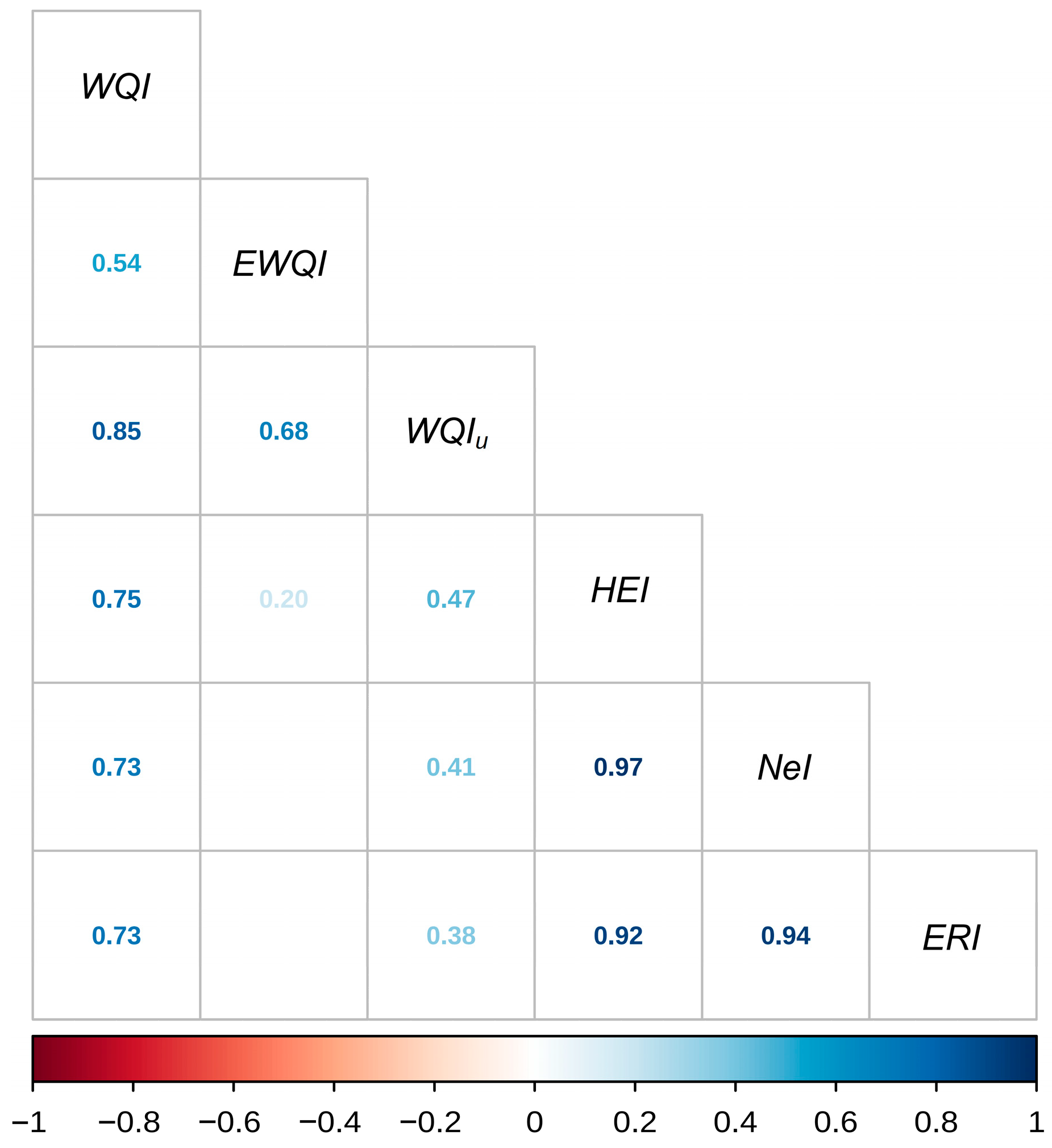
The similarity in behavior of the different $WQIs$ established was analyzed by means of a Sperman correlation matrix, the results of which are shown in Figure 5. It should be noted that the $WQI$ was the index that presented the greatest number of correlations, the highest being with the ${WQI}_u$ (0.85), which would indicate a greater similarity in terms of its results; however, it also presents significant correlations with the indices based on heavy metals. At the same time, it should be noted that the indexes formed by the analysis of heavy metal contamination presented significant correlations between them, since they are formed by the same type of indicators. The $EWQI$ and ${WQI}_u$ indices presented significant correlations between them, but not with respect to the indices based on heavy metals, which could be due to the fact the TDS indicator has a greater weight for these two indices, as can be seen in Figure 3B.

Several studies have developed and analyzed different $WQIs$. Kumar et al. (2024) [42], reviewed a wide variety of $WQIs$ used globally, highlighting the need to adapt these indexes to each region, given the variability in standards and types of pollutants. However, they did not make comparisons or evaluations of their performance. In contrast, Maskooni et al. (2020) [11], compared the $EWQI$ with other indexes such as $HEI$, $NeI$, and $ERI$. They found that most of the wells presented moderate levels of contamination according to these indexes, but without reaching critical values. These results coincide with those of the present study, where $HEI$, $NeI$, and $ERI$ also indicated, for the most part, low contamination, or risk, with some isolated cases of mild or moderate contamination. Unlike other works, the present research directly compares the behavior of the different indexes evaluated with each other, using the $WQI$ based on the indicators recommended by the WHO as the primary reference to analyze the performance and consistency of the results.

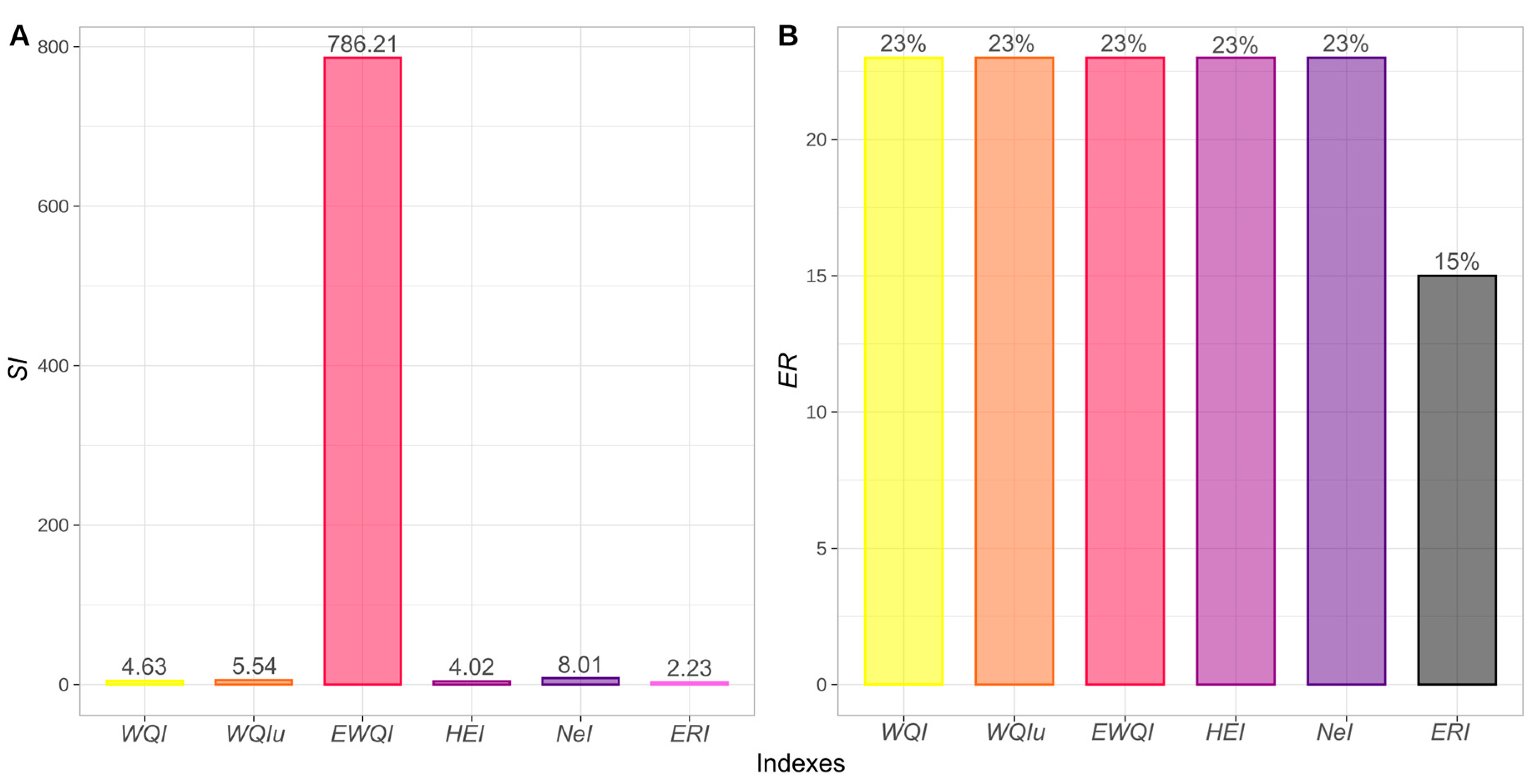
In addition to the above, two criteria were used to evaluate the indexes, the $SI$ and $ER$ indexes, assessments not included in previous investigations, which are shown in Figure 6. Figure 6A measures the precision of the results, while Figure 6B evaluates the relationship between the water quality results and the set of analyzed indicators.

It can be observed that the $EWQI$ presented the worst precision in its results, while the other indexes obtained results in the range of 2.23 to 8.01 (Figure 6A). With respect to the $ER$ index, with the exception of the $ERI$ index, all others presented significant correlations with 23% of the indicators in the database (Figure 6B). With the above, it can be said that the $WQI$, ${WQI}_u$ and $HEI$ indexes presented the best performance with respect to the water quality results obtained. The $EWQI$ and $NeI$ indexes were not as precise, while $ERI$ index showed lower correlation with the analyzed indicators.

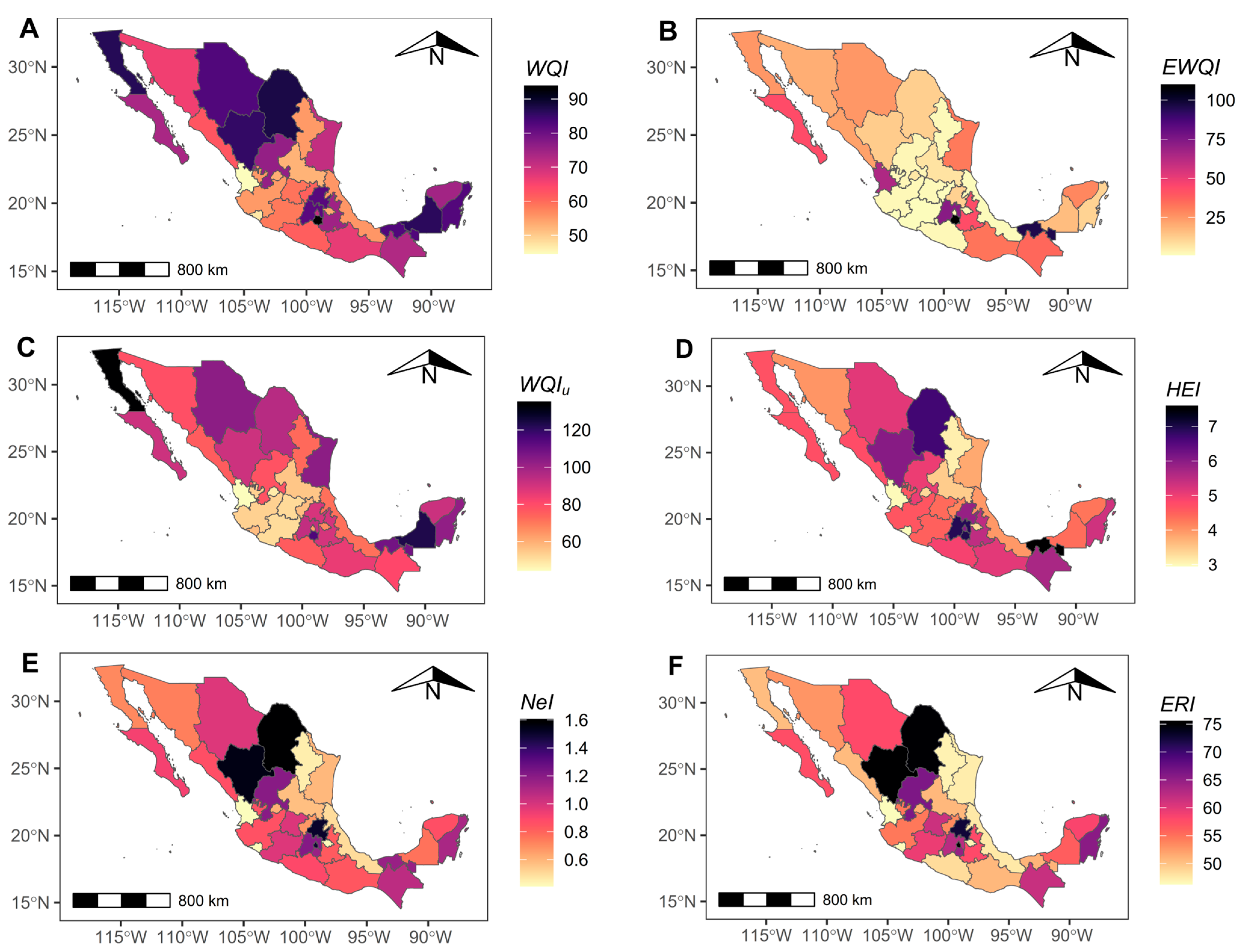
The spatial distribution of quality results of the various $WQIs$ developed is shown in Figure 7. It should be noted that the areas of lowest quality established by the $WQI$, ${WQI}_u$ and $HEI$ indexes are located in the northern (States of Chihuahua, Coahuila, and Durango), northwestern (State of Baja California), center (States of Hidalgo, State of Mexico, Morelos, Tlaxcala, and Mexico city), eastern (State of Tabasco), and peninsula (States of Campeche and Quintana Roo) regions of the country (Figure 7A–C). While the $EWQI$ mostly presents areas of good quality, highlighting the states of Morelos, State of Mexico, Nayarit, and Tabasco as those of lower quality (Figure 7B). The $NeI$ and $ERI$ indices, which analyze the concentration and risk of heavy metal contamination, respectively, presented a similar spatial trend, showing the states of Coahuila, Durango, Hidalgo, and Mexico City as those with the highest levels of contamination and risk, respectively (Figure 7E,F).

3.4. Establishment and Evaluation of ML Models

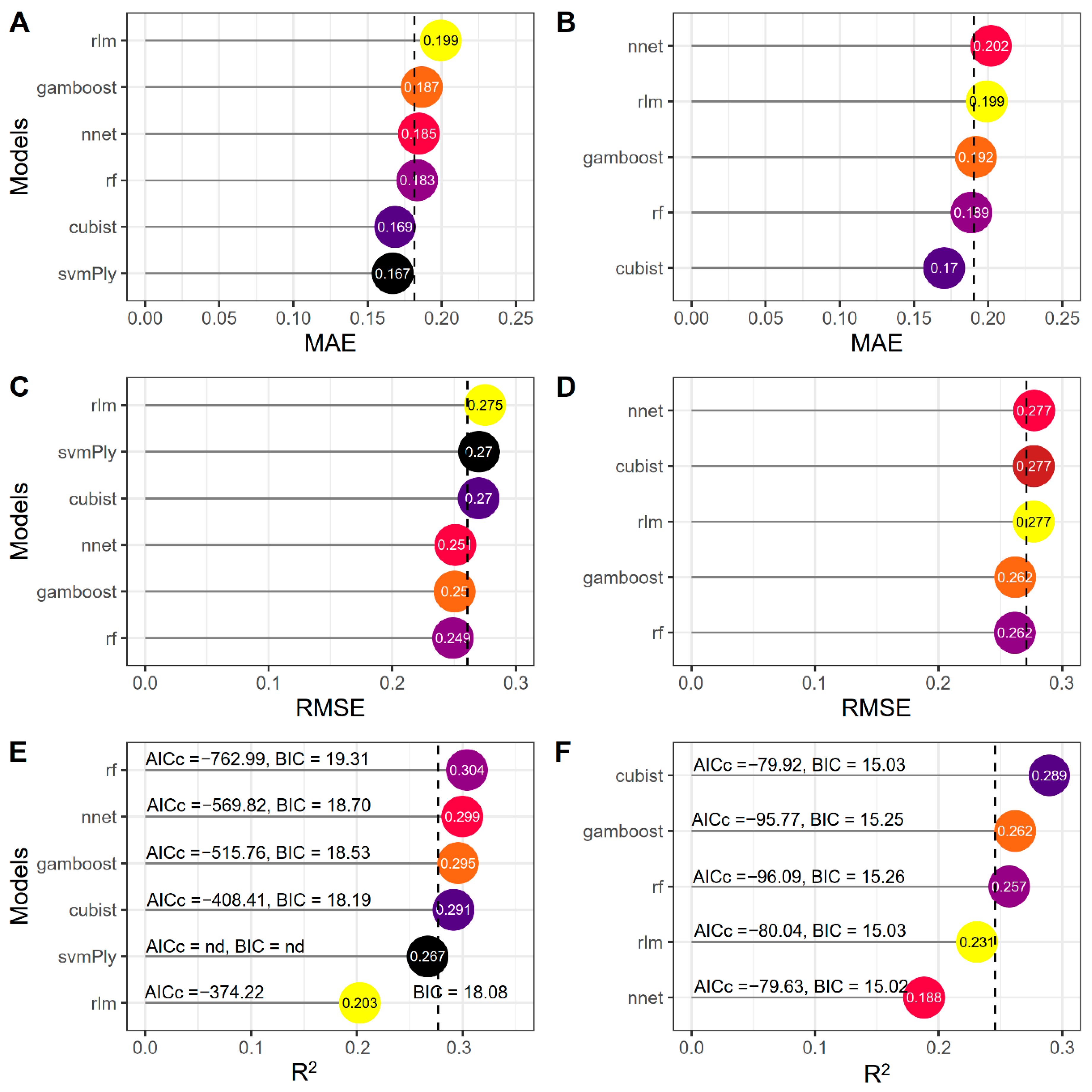
The digital era has led to the advancement of technology to such an extent that the analysis of extensive political, social, commercial, agricultural, and environmental databases makes their interpretation and analysis very difficult, thus creating the need for ML applications that allow obtaining knowledge in a simple way, with the possibility of implementing it for decision-making. This leads to the use of ML models with the purpose of implementation in the analysis and decision-making in environmental approaches, such as water quality. For this reason, the $WQIs$ selected as the best performing in Section 3.3 of this study were evaluated for the establishment and evaluation of six ML models, the results of which are presented in Figure 8, Figure 9 and Figure 10. It should be noted that the $BIC$ and R² evaluation criteria are the most important in selecting the model with the best performance in data prediction.

Regarding the training stage, for the $WQI$, ${WQI}_u$ and $HEI$ indexes, the best performing models were nnt, svmPoly and cubist, respectively (Figure 8A,C,E, Figure 9A,C,E and Figure 10A,C,E, respectively), while for the evaluation phase the best performing models were cubist, svmPoly and cubist, respectively (Figure 8B,D,F, Figure 9B,D,F and Figure 10B,D,F). Regarding the predictive capacity of the models, evaluated from the R² indicator, the one that presented the best performance was the svmPoly model for the ${WQI}_u$ (R² = 0.822, $MAE$ = 0.07, $RSME$ = 0.097, $AICc$ = −376.38, $BIC$ = 19.23) (Figure 9B,D,F), while the one that presented the worst performance was the gamboost model also for the same index (R² = 0.101, $MAE$ = 0.074, $RSME$ = 0.101, $AICc$ = −364.41, $BIC$ = 19.06) (Figure 9B,D,F). It should be noted that the model svmPoly but for the prediction of water quality values for the HEI index did not converge, possibly because said index was composed only of the Cr and Mn indicators, and the low number of data in the test database. The above could serve to select the svmPoly ML model under the analysis of the ${WQI}_u$, as a large-scale monitoring tool for groundwater quality for the different regions of Mexico, reliable and accurate, with the same approach and with results similar to the current $WQI$ used on a global scale and well above the individual analyses of the 13 indicators currently analyzed in the national territory.

Several studies have developed ML models to predict water quality. Kouadri et al. (2021) [24], evaluated eight ML models to estimate $WQI$. In a first scenario, using 12 input indicators, the Multiple Linear Regression (MLR) model showed the highest accuracy (R² = 1, $MAE$ = $1.4\times {10}^{-8}$). However, in a second scenario, with only two indicators, rf model was the most accurate (R² = 0.998, $MAE$ = 1.994). These results highlight the importance of indicator selection on model performance. Sajib et al. (2023) [16], found that Artificial Neural Networks (ANN) outperformed other ML models in terms of sensitivity, with an $RMSE$ = 0.001 and an R² = 1.0, representing exceptional performance. Meanwhile, Eid et al. (2023) [30], reported robust results using Support Vector Machine Regression (SVMR) to predict eight irrigation water quality indexes. The R² values ranged from 0.90 to 0.97 in the training phase, and from 0.88 to 0.95 in the test phase. These findings indicate that SVM is an effective tool for irrigation water quality index ($IWQI$) prediction. The results of this study support previous observations, evidencing the optimal performance of ML models is highly dependent on the data set, the indicators selected and the specific context of the study. This highlights that there is no universal model; the choice of the most appropriate model should be based on the prediction objective and the particular characteristics of the study area. In this sense, the ability of the svmPoly model to capture nonlinear relationships represents a significant advantage.

3.5. Limitations and Recommendations

The development of the $GWQI$-ML model faced several limitations, including the subjectivity inherent in traditional $WQIs$ in the assignment of weights, which can lead to erroneous classifications. It was confirmed that the optimal performance of ML models is highly dependent on the dataset and the context of the study, implying that there is no universal model. One technical limitation observed was the lack of convergence of the svmPoly model for predicting the $HEI$ index, possibly due to the composition of that index (Cr and Mn) and the limited size of the test database (155 elements). In addition, it was noted that the general indices ($EWQI$ and ${WQI}_u$) did not correlate significantly with the heavy metal-based indices, which could be attributed to the greater weight of the TDS indicator in their formulation. Despite these limitations, the study establishes crucial recommendations for water management: the $GWQI$-ML approach should be implemented, using the svmPoly model with the ${WQI}_u$ index, as an objective, accurate, and reliable tool for large-scale monitoring of groundwater quality in Mexico. Fundamentally, it is recommended that CONAGUA adopt the three key indicators (TDS, Cr, and Mn) resulting from the PCA, potentially generating substantial savings in monetary, human, and time resources. Finally, the need to expand the geographical coverage of the studies and promote interdisciplinary collaboration is emphasized, ensuring that the selection of future models is adapted to the prediction objective and the specific characteristics of the study area.

4. Conclusions

The current national groundwater quality assessment in Mexico, which relies on the individual interpretation of 13 quality indicators, is acknowledged as inefficient and costly for CONAGUA in terms of monetary resources, personnel, and time. This study successfully addressed the inherent subjectivity of traditional $WQI$ by developing a novel, objective $GWQI$ through the integration of the $WQI$ conceptual framework and ML models. Crucially, PCA achieved a significant 87% reduction in the number of required indicators, selecting only TDS, Cr, and Mn, which are related to chemical/biological contamination and human health risks, thereby enabling potential resource savings without sacrificing prediction accuracy. Among the evaluated methodologies, the ${WQI}_u$ Index demonstrated the best performance and exhibited a strong correlation ($R^2$ = 0.85) with the widely accepted WHO-based $WQI$, lending credibility to its interpretation. The ML svmPoly model was identified as the most accurate predictor for ${WQI}_u$, achieving a high coefficient of determination ($R^2=$0.822). However, the research confirmed that the optimal performance of ML models is highly dependent on the dataset and context, highlighting that no universal model exists. Based on these findings, we strongly recommend the implementation of the $GWQI$-ML approach using svmPolyas a reliable, accurate, and objective large-scale monitoring tool for Mexican groundwater quality. CONAGUA is advised to adopt the three key indicators (TDS, Cr, Mn) to optimize monitoring resources. The implementation of this model will allow the decision-making of large databases of water quality indicators at the national level, it will possibly allow us to maintain or increase the quality of groundwater bodies.

References

1. Legarreta-González, M.A.; Meza-Herrera, C.A.; Rodríguez-Martínez, R.; Chávez-Tiznado, C.S.; Véliz-Deras, F.G. Time Series Analysis to Estimate the Volume of Drinking Water Consumption in the City of Meoqui, Chihuahua, Mexico. Water 2024, 16, 2634. [Google Scholar] [CrossRef]
2. Mahlknecht, J.; Aguilar-Barajas, I.; Farias, P.; Knappett, P.S.K.; Torres-Martínez, J.A.; Hoogesteger, J.; Lara, R.H.; Ramírez-Mendoza, R.A.; Mora, A. Hydrochemical Controls on Arsenic Contamination and Its Health Risks in the Comarca Lagunera Region (Mexico): Implications of the Scientific Evidence for Public Health Policy. Sci. Total Environ. 2023, 857, 159347. [Google Scholar] [CrossRef]
3. Pacheco-Treviño, S.; Manzano-Camarillo, M.G.F. Review of Water Scarcity Assessments: Highlights of Mexico’s Water Situation. WIREs Water 2024, 11, e1721. [Google Scholar] [CrossRef]
4. Cauich-Kau, D.D.A.; Castro-Larragoitia, J.; Cardona-Benavides, A.; García-Arreola, M.E.; García-Vargas, G.G. An Adapted Groundwater Quality Index Including Toxicological Critical Pollutants. Groundw. Sustain. Dev. 2025, 28, 101401. [Google Scholar] [CrossRef]
5. Roy, P.D.; García-Arriola, O.A.; Selvam, S.; Vargas-Martínez, I.G.; Sánchez-Zavala, J.L. Evaluation of Water from Lake Coatetelco in Central-South Mexico and Surrounding Groundwater Wells for Drinking and Irrigation, and the Possible Health Risks. Environ. Sci. Pollut. Res. 2023, 30, 115430–115447. [Google Scholar] [CrossRef]
6. Bun, S.; Sek, S.; Oeurng, C.; Fujii, M.; Ham, P.; Painmanakul, P. A Survey of Household Water Use and Groundwater Quality Index Assessment in a Rural Community of Cambodia. Sustainability 2021, 13, 10071. [Google Scholar] [CrossRef]
7. Dávalos-Peña, I.; Fuentes-Rivas, R.M.; Fonseca-Montes De Oca, R.M.G.; Ramos-Leal, J.A.; Morán-Ramírez, J.; Martínez Alva, G. Assessment of Physicochemical Groundwater Quality and Hydrogeochemical Processes in an Area near a Municipal Landfill Site: A Case Study of the Toluca Valley. Int. J. Environ. Res. Public Health 2021, 18, 11195. [Google Scholar] [CrossRef] [PubMed]
8. Vázquez-Tapia, I.; Salazar-Martínez, T.; Acosta-Castro, M.; Meléndez-Castolo, K.A.; Mahlknecht, J.; Cervantes-Avilés, P.; Capparelli, M.V.; Mora, A. Occurrence of Emerging Organic Contaminants and Endocrine Disruptors in Different Water Compartments in Mexico—A Review. Chemosphere 2022, 308, 136285. [Google Scholar] [CrossRef] [PubMed]
9. Palma Nava, A.; Parker, T.K.; Carmona Paredes, R.B. Challenges and Experiences of Managed Aquifer Recharge in the Mexico City Metropolitan Area. Groundwater 2022, 60, 675–684. [Google Scholar] [CrossRef]
10. Gao, Y.; Qian, H.; Ren, W.; Wang, H.; Liu, F.; Yang, F. Hydrogeochemical Characterization and Quality Assessment of Groundwater Based on Integrated-Weight Water Quality Index in a Concentrated Urban Area. J. Clean. Prod. 2020, 260, 121006. [Google Scholar] [CrossRef]
11. Maskooni, E.; Naseri-Rad, M.; Berndtsson, R.; Nakagawa, K. Use of Heavy Metal Content and Modified Water Quality Index to Assess Groundwater Quality in a Semiarid Area. Water 2020, 12, 1115. [Google Scholar] [CrossRef]
12. Roy, P.D.; Selvam, S.; Gopinath, S.; Lakshumanan, C.; Muthusankar, G.; Quiroz-Jiménez, J.D.; Zamora-Martínez, O.; Venkatramanan, S. Hydro-Geochemistry-Based Appraisal of Summer-Season Groundwater from Three Different Semi-Arid Basins of Northeast Mexico for Drinking and Irrigation. Environ. Earth Sci. 2021, 80, 529. [Google Scholar] [CrossRef]
13. Farías, P.; Estevez-García, J.A.; Onofre-Pardo, E.N.; Pérez-Humara, M.L.; Rojas-Lima, E.; Álamo-Hernández, U.; Rocha-Amador, D.O. Fluoride Exposure through Different Drinking Water Sources in a Contaminated Basin in Guanajuato, Mexico: A Deterministic Human Health Risk Assessment. Int. J. Environ. Res. Public Health 2021, 18, 11490. [Google Scholar] [CrossRef] [PubMed]
14. Uc-Castillo, J.L.; Marín-Celestino, A.E.; Martínez-Cruz, D.A.; Tuxpan-Vargas, J.; Ramos-Leal, J.A. A Systematic Review and Meta-Analysis of Groundwater Level Forecasting with Machine Learning Techniques: Current Status and Future Directions. Environ. Model. Softw. 2023, 168, 105788. [Google Scholar] [CrossRef]
15. Mahlknecht, J.; Torres-Martínez, J.A.; Kumar, M.; Mora, A.; Kaown, D.; Loge, F.J. Nitrate Prediction in Groundwater of Data Scarce Regions: The Futuristic Fresh-Water Management Outlook. Sci. Total Environ. 2023, 905, 166863. [Google Scholar] [CrossRef]
16. Sajib, A.M.; Diganta, M.T.M.; Rahman, A.; Dabrowski, T.; Olbert, A.I.; Uddin, M.G. Developing a Novel Tool for Assessing the Groundwater Incorporating Water Quality Index and Machine Learning Approach. Groundw. Sustain. Dev. 2023, 23, 101049. [Google Scholar] [CrossRef]
17. Hassan, M.; Hassan, M.; Akter, L.; Rahman, M.; Zaman, S.; Hasib, K.M.; Jahan, N.; Smrity, R.N.; Farhana, J.; Raihan, M.; et al. Efficient Prediction of Water Quality Index (WQI) Using Machine Learning Algorithms. Hum.-Centric Intell. Syst. 2021, 1, 86–97. [Google Scholar] [CrossRef]
18. Juhos, K.; Czigány, S.; Madarász, B.; Ladányi, M. Interpretation of Soil Quality Indicators for Land Suitability Assessment—A Multivariate Approach for Central European Arable Soils. Ecol. Indic. 2019, 99, 261–272. [Google Scholar] [CrossRef]
19. Yu, P.; Liu, S.; Zhang, L.; Li, Q.; Zhou, D. Selecting the Minimum Data Set and Quantitative Soil Quality Indexing of Alkaline Soils Under Different Land Uses in Northeastern China. Sci. Total Environ. 2018, 616–617, 564–571. [Google Scholar] [CrossRef]
20. Bai, Z.; Caspari, T.; Gonzalez, M.R.; Batjes, N.H.; Mäder, P.; Bünemann, E.K.; de Goede, R.; Brussaard, L.; Xu, M.; Ferreira, C.S.S.; et al. Effects of Agricultural Management Practices on Soil Quality: A Review of Long-Term Experiments for Europe and China. Agric. Ecosyst. Environ. 2018, 265, 1–7. [Google Scholar] [CrossRef]
21. Chen, R.-C.; Dewi, C.; Huang, S.-W.; Caraka, R.E. Selecting Critical Features for Data Classification Based on Machine Learning Methods. J. Big Data 2020, 7, 52. [Google Scholar] [CrossRef]
22. Salih Hasan, B.M.; Abdulazeez, A.M. A Review of Principal Component Analysis Algorithm for Dimensionality Reduction. J. Soft Comput. Data Min. 2021, 2, 20–30. [Google Scholar] [CrossRef]
23. Secretaría de Salud [SALUD] NOM-127-SSA1-1994. 1996. Available online: https://www.dof.gob.mx/nota_detalle.php?codigo=2063863&fecha=31/12/1969#gsc.tab=0 (accessed on 27 September 2025).
24. Kouadri, S.; Elbeltagi, A.; Islam, A.R.M.T.; Kateb, S. Performance of Machine Learning Methods in Predicting Water Quality Index Based on Irregular Data Set: Application on Illizi Region (Algerian Southeast). Appl. Water Sci. 2021, 11, 190. [Google Scholar] [CrossRef]
25. Egbueri, J.C.; Enyigwe, M.T. Pollution and Ecological Risk Assessment of Potentially Toxic Elements in Natural Waters from the Ameka Metallogenic District in Southeastern Nigeria. Anal. Lett. 2020, 53, 2812–2839. [Google Scholar] [CrossRef]
26. World Health Organization [WHO]. Guidelines for Drinking-Water Quality: Fourth Edition Incorporating First Addendum, 4th ed.; Incorporating the 1st Addendum; World Health Organization: Geneva, Switzerland, 2017; ISBN 978-92-4-154995-0. [Google Scholar]
27. Nguyen, T.G.; Phan, K.A.; Huynh, T.H.N. Application of Integrated-Weight Water Quality Index in Groundwater Quality Evaluation. Civ. Eng. J. 2022, 8, 2661–2674. [Google Scholar] [CrossRef]
28. Khan, M.B.; Dai, X.; Ni, Q.; Zhang, C.; Cui, X.; Lu, M.; Deng, M.; Yang, X.; He, Z. Toxic Metal Pollution and Ecological Risk Assessment in Sediments of Water Reservoirs in Southeast China. Soil Sediment Contam. Int. J. 2019, 28, 695–715. [Google Scholar] [CrossRef]
29. Singh, P.; Purakayastha, T.J.; Mitra, S.; Bhowmik, A.; Tsang, D.C.W. River Water Irrigation with Heavy Metal Load Influences Soil Biological Activities and Risk Factors. J. Environ. Manag. 2020, 270, 110517. [Google Scholar] [CrossRef]
30. Eid, M.H.; Elbagory, M.; Tamma, A.A.; Gad, M.; Elsayed, S.; Hussein, H.; Moghanm, F.S.; Omara, A.E.-D.; Kovács, A.; Péter, S. Evaluation of Groundwater Quality for Irrigation in Deep Aquifers Using Multiple Graphical and Indexing Approaches Supported with Machine Learning Models and GIS Techniques, Souf Valley, Algeria. Water 2023, 15, 182. [Google Scholar] [CrossRef]
31. R Core Team. R: Language and Environment for Statistical Computing; R Foundation for Statistical Computing: Vienna, Austria, 2021. [Google Scholar]
32. Kuhn, M. Caret: Classification and Regression Training, Version 6.0-94; R Foundation for Statistical Computing: Vienna, Austria, 2007. [Google Scholar]
33. Arias-Rodriguez, L.F.; Tüzün, U.F.; Duan, Z.; Huang, J.; Tuo, Y.; Disse, M. Global Water Quality of Inland Waters with Harmonized Landsat-8 and Sentinel-2 Using Cloud-Computed Machine Learning. Remote Sens. 2023, 15, 1390. [Google Scholar] [CrossRef]
34. Chicco, D.; Warrens, M.J.; Jurman, G. The Coefficient of Determination R-Squared Is More Informative than SMAPE, MAE, MAPE, MSE and RMSE in Regression Analysis Evaluation. PeerJ Comput. Sci. 2021, 7, e623. [Google Scholar] [CrossRef]
35. Zhang, J.; Yang, Y.; Ding, J. Information Criteria for Model Selection. WIREs Comput. Stats 2023, 15, e1607. [Google Scholar] [CrossRef]
36. Colín Carreño, M.A.; Esquivel Martínez, J.M.; Salcedo Sánchez, E.R.; Álvarez Bastida, C.; Padilla Serrato, J.G.; Lopezaraiza Mikel, M.E.; Talavera Mendoza, Ó. Human Health Risk and Quality Assessment of Spring Water Associated with Nitrates, Potentially Toxic Elements, and Fecal Coliforms: A Case from Southern Mexico. Water 2023, 15, 1863. [Google Scholar] [CrossRef]
37. Santacruz-De León, G.; Moran-Ramírez, J.; Ramos-Leal, J.A. Impact of Drought and Groundwater Quality on Agriculture in a Semi-Arid Zone of Mexico. Agriculture 2022, 12, 1379. [Google Scholar] [CrossRef]
38. Gutiérrez, M.; Alarcón-Herrera, M.T. Fluoruro en aguas subterráneas de la región centro-norte de México y su posible origen. Rev. Int. Contam. Ambient. 2022, 38, 389–397. [Google Scholar] [CrossRef]
39. Morales-deAvila, H.; Gutiérrez, M.; Colmenero-Chacón, C.P.; Júnez-Ferreira, H.E.; Esteller-Alberich, M.V. Upward Trends and Lithological and Climatic Controls of Groundwater Arsenic, Fluoride, and Nitrate in Central Mexico. Minerals 2023, 13, 1145. [Google Scholar] [CrossRef]
40. Ramos, E.; Bux, R.K.; Medina, D.I.; Barrios-Piña, H.; Mahlknecht, J. Spatial and Multivariate Statistical Analyses of Human Health Risk Associated with the Consumption of Heavy Metals in Groundwater of Monterrey Metropolitan Area, Mexico. Water 2023, 15, 1243. [Google Scholar] [CrossRef]
41. Ramírez-Cota, M.; Escobar-Sánchez, O.; Betancourt-Lozano, M.; Frías-Espericueta, M.G.; Zamora-Arellano, N.Y.; Osuna-Martínez, C.C. Heavy Metals in Drinking Water Sources in Northern Mexico: A Review of Concentrations and Human Health Risks Assessment. J. Water Health 2025, 23, 684–700. [Google Scholar] [CrossRef]
42. Kumar, D.; Kumar, R.; Sharma, M.; Awasthi, A.; Kumar, M. Global Water Quality Indices: Development, Implications, and Limitations. Total Environ. Adv. 2024, 9, 200095. [Google Scholar] [CrossRef]
Figure 1. Study area and regions of Mexico.
Hydrology 12 00285 g001
Figure 2. Process diagram. W Q I , water quality index; E W Q I , entropy weighted water quality index; W Q I u , unified water quality index; H E I , heavy metal evaluation index; N e I , nemerow index; E R I , ecological risks of heavy metals; TDS, total dissolved solids; Cr, crome; Mn, manganese; gamboost, boosted generalized additive model; cubist, decision trees and multiple linear regression methods; rf, random forest; nnet, neural network; rlm, robust linear model; svmPoly, support vector machines with polynomial kernel; M A E , mean absolute error; R M S E , root mean square error; A I C c , Akaike information criterion corrected; B I C , Bayesian information criterion; R2, coefficient of determination.
Hydrology 12 00285 g002
Figure 3. Bi-graph of PCs (A) and Spearman correlation matrix of indicators and PCs (B). PCs, principal components; EC, electrical conductivity; TDSs, total dissolved solids; HRD, hardness; Cr, chromium; Mn, manganese.
Hydrology 12 00285 g003
Figure 4. Spatial distribution of indicators resulting from the PCA. TDS (A), total dissolved solids; Cr (B), chromium; Mn (C), manganese.
Hydrology 12 00285 g004
Figure 5. Spearman correlation matrix of analyzed indixes. W Q I , water quality index; E W Q I , entropy weighted water quality index; W Q I u , unified water quality index; H E I , heavy metal evaluation index; N e I , nemerow index; E R I , ecological risks of heavy metals in groundwater.
Hydrology 12 00285 g005
Figure 6. Sensitivity index (A) and efficiency rate index (B) of developed quality indices. W Q I , water quality index; E W Q I , entropy weighted water quality index; W Q I u , unified water quality index; H E I , heavy metal evaluation index; N e I , nemerow index; E R I , ecological risks of heavy metals in groundwater.
Hydrology 12 00285 g006
Figure 7. Spatial distribution of quality values of developed quality indices. (A) W Q I , water quality index; (B) E W Q I , entropy-weighted water quality index; (C) W Q I u , unified water quality index; (D) H E I , heavy metal evaluation index; (E) N e I , nemerow index; (F) E R I , ecological risks of heavy metals in groundwater.
Hydrology 12 00285 g007
Figure 8. Evaluation criteria for the ML models developed for the W Q I . (A,C,E), training stage criteria. (B,D,F), evaluation stage criteria. W Q I , water quality index; gamboost, boosted generalized additive model; cubist, decision trees and multiple linear regression methods; rf, random forest; nnet, neural network; rlm, robust linear model; svmPoly, support vector machines with polynomial kernel; M A E , mean absolute error; R M S E , root mean square error; A I C c , Corrected Akaike information criterion; B I C , Bayesian information criterion; R2, coefficient of determination; Dotted line, mean value of the criterion.
Hydrology 12 00285 g008
Figure 9. Evaluation criteria for the ML models developed for the W Q I u . (A,C,E), training stage criteria. (B,D,F), evaluation stage criteria. W Q I u , unified water quality index; gamboost, boosted generalized additive model; cubist, decision trees and multiple linear regression methods; rf, random forest; nnet, neural network; rlm, robust linear model; svmPoly, support vector machines with polynomial kernel; M A E , mean absolute error; R M S E , root mean square error; A I C c , Corrected Akaike information criterion; B I C , Bayesian information criterion; R2, coefficient of determination; Dotted line, mean value of the criterion.
Hydrology 12 00285 g009
Figure 10. Evaluation criteria for the ML models developed for the H E I . (A,C,E), training stage criteria. (B,D,F), evaluation stage criteria. H E I , heavy metal evaluation index; gamboost, boosted generalized additive model; cubist, decision trees and multiple linear regression methods; rf, random forest; nnet, neural network; rlm, robust linear model; svmPoly, support vector machines with polynomial kernel; M A E , mean absolute error; R M S E , root mean square error; A I C c , Corrected Akaike information criterion; B I C , Bayesian information criterion; R2, coefficient of determination; Dotted line, mean value of the criterion.
Hydrology 12 00285 g010