Article

Short-Term Drought Forecast across Two Different Climates Using Machine Learning Models

by
Reza Piraei
1,
Majid Niazkar
2,3,*,
Fabiola Gangi
4,
Gökçen Eryılmaz Türkkan
5 and
Seied Hosein Afzali
1
1
Department of Civil Engineering, Shiraz University, Shiraz 7134851156, Iran
2
Euro-Mediterranean Center on Climate Change, Porta dell’Innovazione Building, 2nd Floor Via della Libertà 12, Marghera, 30175 Venice, Italy
3
Ca’ Foscari University of Venice, 30123 Venice, Italy
4
Department of Agriculture and Environmental Sciences, University of Milan, Via Celoria 2, 20133 Milano, Italy
5
Department of Civil Engineering, Balıkesir University, 10145 Balıkesir, Türkiye
*
Author to whom correspondence should be addressed.
Hydrology 2024, 11(10), 163; https://doi.org/10.3390/hydrology11100163
Submission received: 10 August 2024 / Revised: 28 September 2024 / Accepted: 29 September 2024 / Published: 3 October 2024
(This article belongs to the Special Issue Hydrological Modeling and Sustainable Water Resources Management)

Abstract

:
This paper presents a comparative analysis of machine learning (ML) models for predicting drought conditions using the Standardized Precipitation Index (SPI) for two distinct stations, one in Shiraz, Iran and one in Tridolino, Italy. Four ML models, including Artificial Neural Network (ANN), Multiple Linear Regression, K-Nearest Neighbors, and XGBoost Regressor, were employed to forecast multi-scale SPI values (for 6-, 9-, 12-, and 24-month) considering various lag times. Results indicated that the ML model with the most robust performance varied depending on station and SPI duration. Furthermore, ANN demonstrated robust performance for SPI estimations at Shiraz station, whereas no single model consistently outperformed the others for Tridolino station. These findings were further validated through the confidence percentage analysis performed on all ML models in this study. Across all scenarios, longer SPI durations generally yielded better model performance. Additionally, for Shiraz station, optimal lag times varied by SPI duration: 6 months for the 6- and 9-month SPI, 4 months for the 12-month SPI, and 2 months for the 24-month SPI. For Tridolino station, on the other hand, no definitive optimal lag time was identified. These findings contribute to our understanding of predicting drought indicators and supporting effective water resource management and climate change adaptation efforts.

1. Introduction

Climate change refers to long-term shifts in the Earth’s weather patterns and average temperatures [1]. It is primarily caused by human activities, particularly the burning of fossil fuels (such as coal, oil, and natural gas), which release greenhouse gases into the atmosphere. The consequences of climate change have impacts on various aspects of our planet. Some of the most important effects include rising temperatures, melting ice, rising sea levels, extreme weather events, ecosystem disruptions, and drought.
Drought is a natural hazard posing significant challenges to water resources, agriculture, and ecosystem health. For drought analysis, some drought indices have been recommended to delineate whether a basin experiences drought.
The Standardized Precipitation Index (SPI) is a widely used climate index that measures the deviation of precipitation from its long-term average [2,3]. It basically provides a standardized measure of drought or wetness conditions based on precipitation data. In other words, SPI is a statistical tool that transforms precipitation values into a dimensionless index, enabling comparisons across different locations and time periods. The magnitude of the SPI represents the severity of the deviation from the long-term average, with more extreme values indicating more severe drought or wetness. Typically, it is calculated over different time scales, such as 1 month, 3 months, 6 months, 12 months, etc., which allows assessment of short-term or long-term drought conditions. For example, a negative SPI value over a 12-month time scale demonstrates a prolonged period of below-average precipitation and could indicate long-term drought. Therefore, the SPI is a valuable tool for monitoring and assessing drought conditions, identifying drought onset and duration, and comparing drought severity across different regions, which is the scope of this study. Hence, SPI-based drought analysis is indeed one of the important tasks in water resources management and climate change impact assessment studies.
There has been increasing interest in using machine learning (ML) algorithms for conducting climate change research. ML techniques build an estimation model based on sample data, known as training data, to make predictions or decisions without being explicitly programmed to do so. They have shown results in improving the accuracy and efficiency of climate models, enabling faster analysis of large datasets and supporting the development of predictive models for future climate scenarios.
There are many studies in the literature focusing on SPI-based drought analysis using ML models (Table 1). For instance, Hosseini-Moghari and Araghinejad [4] investigated drought-forecasting SPI in the Gorganroud basin over various time scales (3, 6, 9, 12, and 24 months). They utilized neural networks, including a Recursive Multi-Step Multi-Layer Perceptron and the Direct Multi-Step Radial Basis Function. They found that recursive models performed better for smaller SPI time scales, whereas direct models exhibited better accuracy with longer SPI durations. Furthermore, Docheshmeh Gorgij et al. [5] investigated the effectiveness of long short-term memory (LSTM) in forecasting drought using monthly rainfall data of four stations in Iran. They reported that LSTM outperformed Extra Trees (ET), Vector Autoregressive (VAR), and Multivariate Adaptive Regression Spline (MARS) methods in forecasting SPI values at different time scales (3, 6, 9, and 12 months). Moreover, Lotfirad et al. [6] aimed to select the best model for predicting SPI values with time scales of 1, 3, 6, 9, 12, 24, and 48 months using Random Forest (RF) with lag times ranging from 1 to 12 months. They concluded that the best set of lag times is different for each station and time scale of SPI. Piri et al. [7] evaluated various ML models, including Artificial Neural Network (ANN) and Support Vector Regression (SVR), optimized by Particle Swarm Optimization and Response Surface Method (RSM), for predicting meteorological drought indices. According to their study, SVR-RMS emerged as the best model for accuracy in forecasting drought indices. Additionally, Shakeri et al. [8] estimated SPI values for meteorological and hydrological drought assessment in Yazd, Iran. They focused on SPI values with time scales of 3, 6, 12, and 24 months. They employed linear and non-linear ML models, with RF indicating the highest accuracy in predicting SPI values at different time scales. Furthermore, Elbeltagi et al. [9] conducted a study in Rajasthan, India, evaluating various ML models for predicting SPI values at 3, 6, and 12-month intervals. They compared the performance of Random Subspace (RSS) models alone and combined with M5 Pruning Tree (M5P), RF, and Random Tree (RT). Their results demonstrated that the hybrid RSS-M5P model outperformed others in predicting SPI values, highlighting the effectiveness of RSS-M5P in drought estimation for agricultural applications. Similarly, Elbeltagi et al. [10] focused on drought prediction in Maharashtra, India, using RF, RT, and Gaussian process regression (GPR-PUK kernel) models. By analyzing SPI data at 6- and 12-month intervals, they found RF to be the most robust model for forecasting drought events at meteorological stations in the upper basin area of the Godavari River. In addition, Coşkun and Citakoglu [11] investigated drought prediction in Sakarya province, Türkiye, using LSTM networks. By analyzing the SPI data at various time scales, they compared the performance of LSTM with that of an Empirical Mode Decomposition (EMD)–Extreme Learning Machine (ELM) hybrid model. Based on their results, LSTM exhibited excellent SPI predictions, particularly for shorter time scales of SPI. Furthermore, Adnan et al. [12] evaluated the prediction accuracy of heuristic ML methods, including Optimally Pruned ELM (OP-ELM) and a Dynamic Evolving Neural-Fuzzy Inference System (DENFIS), for drought modeling in Pakistan. Their study focused on SPI at different time scales across multiple meteorological stations. According to their results, DENFIS outperformed other models in most cases, showing its effectiveness in drought analysis with improved accuracy, particularly for shorter SPI time scales. Moreover, Saha et al. [13] proposed an ensemble ML approach for assessing drought vulnerability in Odisha, India, using M5P, M5P-Dagging, M5P-RSS, and M5P-Rotation Forest (M5P-RTF) models. By incorporating various drought vulnerability indicators, they demonstrated the capability of ensemble models to produce accurate drought vulnerability maps. Among the ensemble models, M5P-RFT exhibited the highest accuracy in their study. Finally, Niazkar et al. [14] examined the trend changes in the SPI values at 6, 9, 12, and 24 months, using innovative trend analysis. Additionally, they applied Multiple Linear Regression (MLR), ANN, K-Nearest Neighbors (KNN), and XGBoost Regressor (XGBR) using rainfall data for between 1965 and 2020 from eight rainfall stations. Despite the abundance of the literature exploring ML models for SPI-based drought analysis, there remains a noticeable gap in the literature concerning comparative assessments of these models across different geographical regions. Furthermore, while previous studies have highlighted the effectiveness of certain ML algorithms for SPI prediction, there is still a need for comprehensive evaluations encompassing a wide range of ML techniques in order to identify the most suitable approach for each station and time scale.
The aim of this study was to evaluate drought conditions in two different climates, i.e., at one station in a semi-arid region (Shiraz, Iran) and one station in a Mediterranean region (Tridolino, Italy). For this purpose, four ML models were exploited to forecast 6-, 9-, 12-, and 24-month SPI values for the selected rainfall stations. Various SPI lag times ranging from 1 to 6 were utilized as input variables for ML models. By examining numerous case scenarios, this study not only offers valuable insights into the drought status of both study areas but also provides a comprehensive comparative analysis of different ML models for SPI predictions. Building upon the emphasis of previous studies on comparative analysis [14], this study underscores the importance of evaluating diverse ML approaches across distinct geographical locations to enhance the understanding and applicability of ML models in drought analysis. Moreover, this study focuses on two stations from geographically different regions, Iran and Italy, thereby providing a better understanding of the applicability of ML models across diverse climatic conditions. Furthermore, feature importance analysis was conducted on the ML models to highlight the significance of each lag time in the final predictions. Finally, confidence percentages were calculated to evaluate the predictive capability and reliability of ML models for future SPI predictions.

2. Materials and Methods

2.1. Study Areas

This study considered two case studies from two countries, involving two different climate conditions. The details of these cases are presented below.
(1) Shiraz station: Rainfall data measured at the synoptic station in Shiraz, Fars province, Iran were utilized in this study. The location of Shiraz and the corresponding station are depicted in Figure 1. As shown, the latitude of the station is at 29°48′ N, 29°29′ S, while its longitude is 52°40′ E and 52°23′ W. The average annual rainfall from 1923 to 2015 was 274.7 mm per year. Shiraz’s climate is temperate because its average altitude is 1484 m above sea level. The maximum, minimum, and average temperatures in Shiraz are 40.2, 14.4, and 18 °C, respectively.
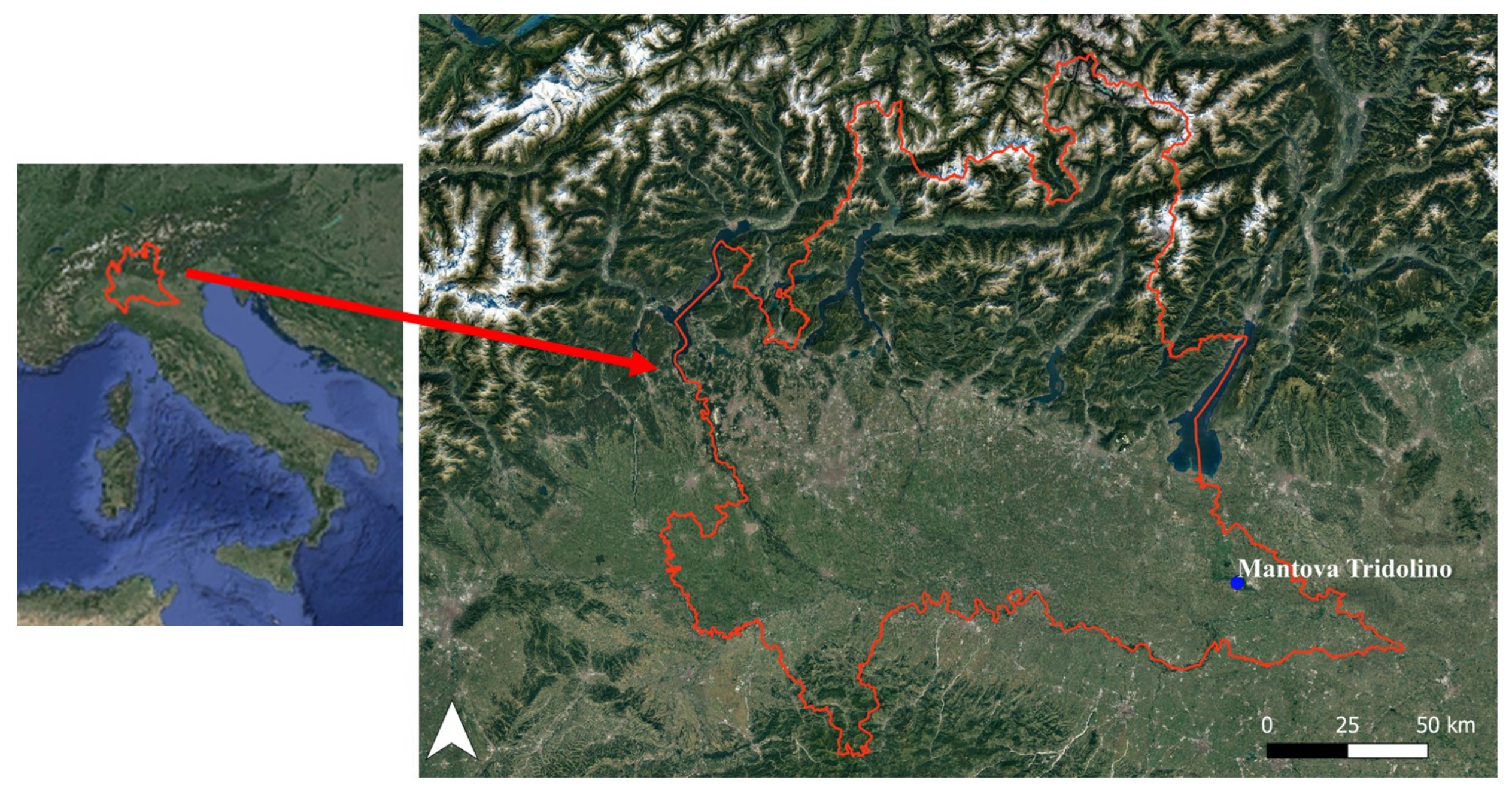
(2) Tridolino station: The Mantova Tridolino pluviometric station is in the Lombardy region, south of Lake Garda, Italy (Figure 2). Strategically located in the heart of the Po Valley, one of the most water-rich regions in Europe, characterized by a complex network of rivers, canals, and springs, this station is an integral part of the regional meteorological and hydrological observation system. Thus, it is an important node in the hydrological monitoring network of the area. It contributes significantly to the understanding of rainfall patterns and water flows in the surrounding area. The data analyzed from this station covered the period from 1993 to 2023.
Table 2 presents the statistical characteristics of the data collected from both stations. To be more specific, it provides the minimum, maximum, average, skewness, and standard deviation of precipitation and SPI values for 6, 9, 12, and 24 months for Shiraz station (1927–2017) and Tridolino station (1993–2023). As shown, the average rainfall measured at Shiraz station (26.81 mm) has been lower than the mean rainfall at Tridolino station (40.07 mm), whereas the maximum rainfall observed at Shiraz station (330 mm) was approximately twice as high as the maximum rainfall at Tridolino station (159.36). Furthermore, Table 2 reveals that both stations have reported a wide range of SPI values across different time scales.

2.2. Standardized Precipitation Index

SPI is one of the most popular drought indices [29,30]. In this index, the rainfall data may be fitted by a gamma distribution, and consequently, SPI is calculated using the gamma distribution, as shown in Equation (1):
f x ; α , β = 1 β α τ ( α ) x α 1 e x / β   f o r   x ,   α ,   β   >   0
where β, α, x, and τ(α) represent the scale, shape variables, rainfall amount, and gamma function, respectively. The most precise values of α and β can be obtained by Equations (2) and (3), respectively [14]:
α = 1 4 A 1 + 1 + 4 A 3
β = x ¯ α
where A = l n x ¯ l n ( x ) n , and x ¯ and n are the mean rainfall and quantity of data, respectively.
In this study, the rainfall data of each station was checked to see whether it followed the gamma distribution. The results of the statistical tests indicated that the rainfall data for the two stations were consistent with the gamma distribution. The Kolmogorov-Smirnov test did not reject the null hypothesis in either case, with p-values of 0.5436 for the Mantova Tridolino station and 0.099592 for Shiraz station (after removing data with zero precipitation), respectively. Therefore, the observed rainfall data followed a gamma distribution, confirming the applicability of the SPI calculation.
When the SPI is between −0.99 and 0.99, the drought status is normal. In addition, positive SPI values higher than 1 indicate wetter-than-average conditions: (i) moderately wet (1.00 < SPI < 1.49), (ii) very wet (1.50 < SPI < 1.99), and (iii) extremely wet (SPI  >  2.00). On the other hand, negative SPI values lower than 1 denote drier-than-average conditions: (i) moderately dry (−1.00 < SPI < −1.49), (ii) severely dry (−1.50 < SPI < −1.99), and (iii) extremely dry (SPI < −2.00).

2.3. Machine Learning Models

This study utilized four ML models for predicting the SPI across diverse timeframes. The Python programming language was employed to implement ML models, specifically using the Scikit-learn library for coding MLR and KNN models, the XGboost library for implementing eXtreme Gradient Boosting (XGBoost) models, and the Keras library with TensorFlow as the backend for applying ANNs. Preceding model implementation, the dataset was modified to enhance the models’ performances, incorporating the utilization of the MinMaxScaler technique from the Scikit-learn library. The rescaling involved adjusting each variable within a range of 0 to 1. Subsequently, the data were randomly divided into two groups: (i) 80% for training dataset and (ii) the remainder as a test dataset. Furthermore, the dataset for each station was handled separately, and the ML models were trained on the Shiraz and Tridolino data to assess their performances in predicting the SPI under each distinct climate condition. To optimize model performances, hyperparameter tuning was performed for each ML model, using a grid search method [31]. Table 3 provides the key hyperparameters tuned for each ML model [32,33,34]. The subsequent section outlines each ML model individually.

2.3.1. Artificial Neural Networks

ANNs stand out among various types of neural networks described in previous studies on drought analysis [35]. They represent a widely utilized ML model that bears a resemblance to the human brain, consisting of interconnected units known as neurons or nodes. In the architecture of any neural network, the output of a neuron serves as the input for the subsequent one. The weighted values received by each neuron are added together, while an activation function is generally used to limit the amplitude of the neuron output. In this study, the tanh activation function was used for hidden layers, whereas a linear function was employed for the output layer.
In this study, the number of input neurons in each model varied from 1 to 6 based on lead times, and a single hidden layer was considered. Furthermore, consistent with a recommendation from a prior study [14], the number of hidden neurons was set to 2m + 1, where m denotes the number of input neurons. Finally, the ANN models were trained using 500 epochs, and an early stopping criterion was implemented. To be more specific, if the error failed to decrease after 100 epochs, the algorithm halted the training process, returning the weights and biases corresponding to the minimum error.

2.3.2. eXtreme Gradient Boosting Regressor

XGBR is a tree-based boosting ML technique recognized for its performance, speed, scalability, and unique features in addressing both regression and classification problems [14]. As a variation of the gradient boosting model, its simplicity, parallelism, and outstanding predictive accuracy have led to victories in various ML competitions [36]. Essentially, XGBoost integrates multiple weak learning models (i.e., decision trees) and refines their residuals iteratively, making it highly effective for sparse data. It exploits a sparsity-aware split-finding approach, processes large datasets efficiently through its block technology, and employs CPU multithreading for parallelism, setting it apart with distinctive capabilities in handling large-scale data [37]. In contrast to conventional ML models like RF, XGBR establishes a sequence of consecutive decision trees by leveraging prediction errors (residuals) from the preceding trees. It entails a dependency among the trees, with each new tree constructed based on the most recent residuals of the previous one. The final output for each sample is represented by the cumulative weighted output values of the trees [38]. Additionally, the unique objective function of XGBoost incorporates both training error and regularization components, helping to minimize overfitting and improve generalization performance. These advancements contribute to its superior performance, particularly in applications like hydrological modeling, water quality prediction, and groundwater management [37].

2.3.3. K Nearest Neighbors

Data-driven techniques are useful for deriving significant insights, such as hidden patterns, correlations, and trends, from large datasets by using advanced mathematical functions and algorithms. Among ML models, KNN stands out as a popular nonparametric approach for (i) regression models and (ii) pattern classification [39]. It is often referred to as a “lazy learner” because it does not require a training phase. Instead, it stores the entire training dataset and performs calculations only at runtime, making it computationally efficient for smaller datasets. However, it may become slower for larger datasets due to its reliance on real-time calculations of distance [40]. It predicts test data points based on the classifications of their K nearest neighbors within the training data, demonstrating robustness in handling various combinations, mitigating overfitting risks, effectively managing large datasets, and exhibiting resilience to noisy data [41]. Furthermore, the distances between test and training data points are calculated using distance functions, such as the Minkowski distance function described by Equation (4):
d X t r , X t e = i = 1 n x t r i x t e i p 1 p
where X t r and X t e represent the training data with specific parameters ( x t r 1 , x t r 2 , , x t r n ) and the test data with specific parameters ( x t e 1 ,   x t e 2 , , x t e n ), respectively, and p is the power of the Minkowski distance function. If p = 1, the distance function is referred to as Manhattan, while if p = 2, it is called Euclidean.
Subsequently, the distances in KNN are sorted and the nearest neighbor is identified based on the minimum distance, signifying the maximum similarity. The prediction process involves finding the K nearest data points, calculating the weighted average target values, and determining the output for a given data point. The choice of K in KNN significantly influences model accuracy, with a low K resulting in inaccurate predictions and a high K potentially leading to overfitting [14].

2.3.4. Multiple Linear Regression

The foundation of MLR rests on the presumption of a linear association between the dependent variable (output data, denoted as y ) and independent variables (input data, denoted as x i ) [14]. In this context, Equation (5) embodies the structure of an MLR model:
y = β 0 + i = 1 n 1 β i x i
where β 0 is a constant, signifying the y-axis intersection point of the regression line. The β i values symbolize the slopes of lines linking the regression line to individual data points. Finally, the parameter n 1 denotes the number of independent variables.

2.4. Feature Importance Analysis

After tuning and implementing XGBR, feature importance analysis, akin to sensitivity analysis, was performed using a built-in function within XGBoost to rank the influence of each input feature on the model’s predictions. Typically, this type of assessment employs metrics such as a weight or a gain to evaluate the feature importance [31]. To be more specific, the weight reflects the frequency of each feature’s usage in splitting the data across all trees, while the gain computes the average improvement in accuracy attained when each feature is utilized for data splitting. In this study, the gain was utilized. Finally, features with a higher importance, i.e., a stronger influence, can inform subsequent analyses or feature selection endeavors.

2.5. Performance Criteria

To assess various ML models, four distinct criteria were employed: (i) root mean square error (RMSE), (ii) mean absolute error (MAE), (iii) Nash-Sutcliffe efficiency (NSE), and (iv) the determination coefficient (R2). The equations of these metrics are presented as follows [14]:
R M S E = i = 1 n O i P i 2 n
M A E = 1 n i = 1 n O i P i
N S E = 1 i = 1 n O i P i 2 i = 1 n O i i = 1 n O i n 2
R 2 = i = 1 n O i i = 1 n O i n P i i = 1 n P i n i = 1 n O i i = 1 n O i n 2 i = 1 n P i i = 1 n P i n 2 2
where O i and P i denote the ith observed and predicted SPIs, respectively.
According to the definition of each metric, it is evident that an enhancement in the accuracy of SPI estimations is associated with higher values of R2 and NSE, along with lower values of RMSE and MAE.

2.6. Confidence Percentages Analysis

According to the SPI definition in Section 2.2, each data point represented a condition ranging from extremely dry to extremely wet. Based on this classification, the actual SPI values and those predicted by each ML model were categorized in different drought classes. A value of 1 was assigned when both predicted and observed SPI values fell into the same category. Otherwise, a value of 0 was given. The average of these values as a percentage yielded a confidence percentage (CP) related to the drought index. CP results can reveal for how many points (in percentage) an ML model estimates the correct class of SPI [42].

3. Results and Discussion

3.1. Results of Comparing Different Models in Terms of Metrics

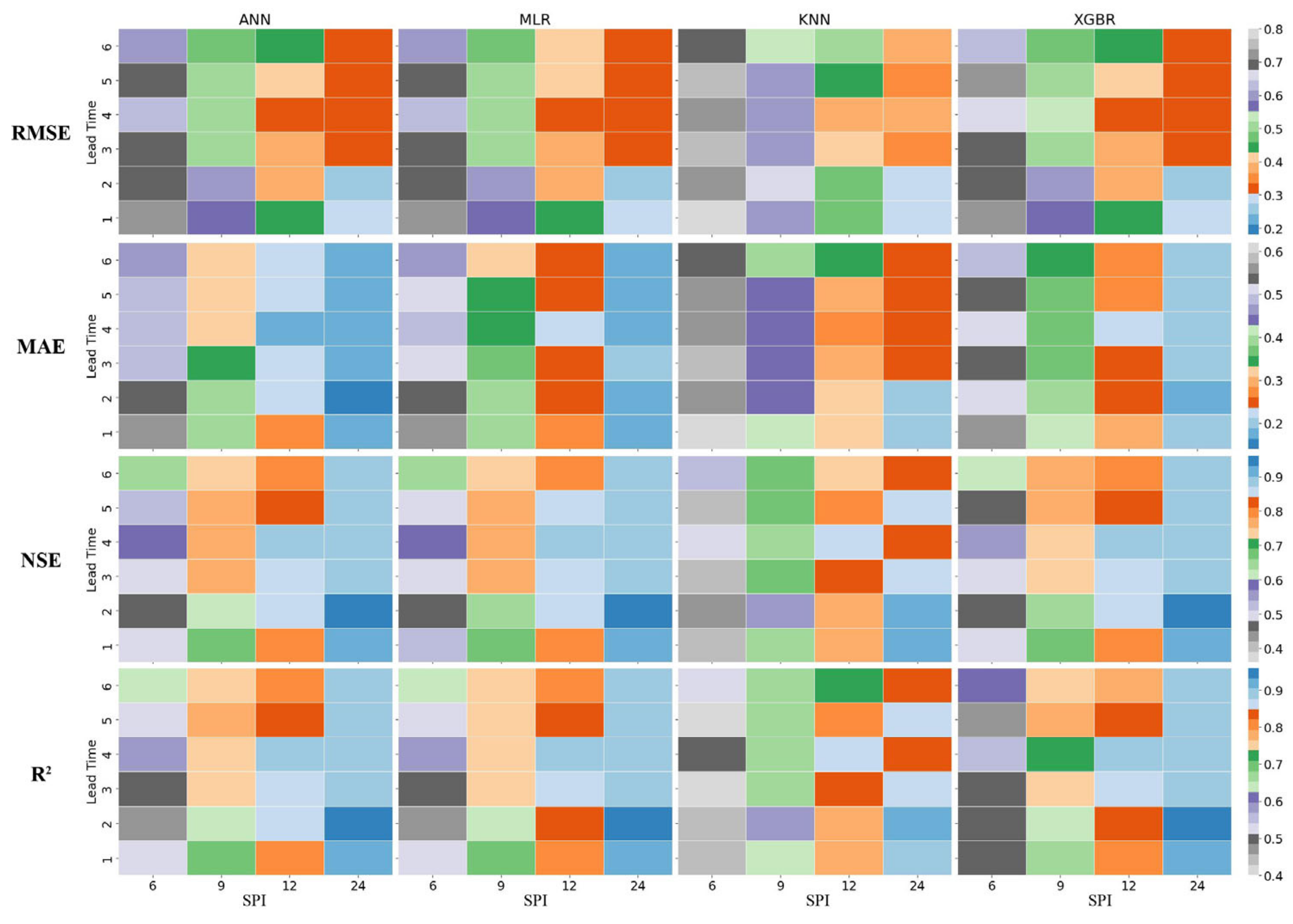
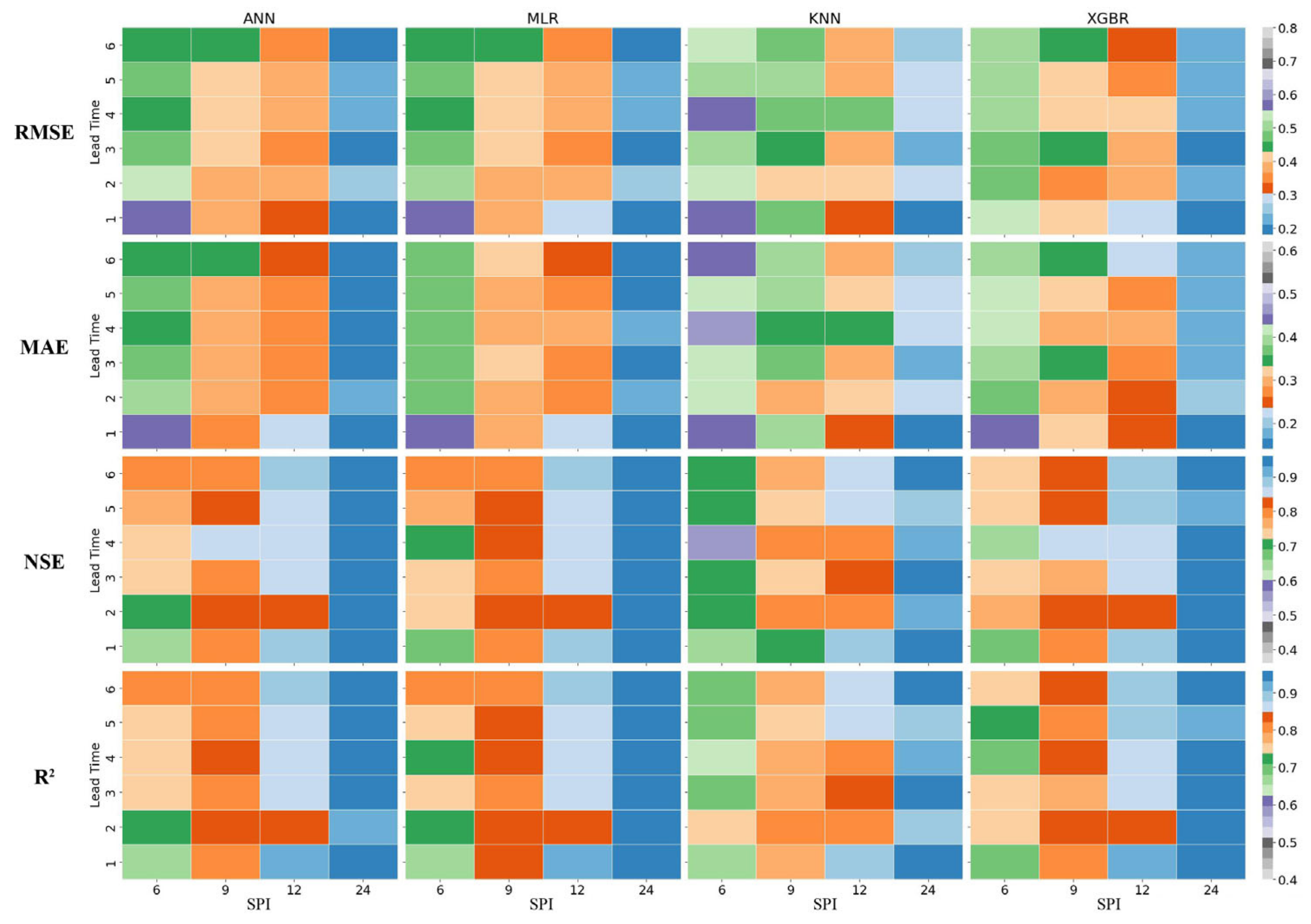
This study employed four ML models to forecast the 6-, 9-, 12-, and 24-month SPI values across two stations from two different countries, while accounting for six different lag times. Consequently, a total of 192 cases (four ML models × four SPIs × two case studies × six lag times) were developed and compared. To facilitate a comprehensive evaluation, the ML models for each station are presented individually as distinct case studies. The metric outcomes for Shiraz and Tridolino stations are depicted in Figure 3 and Figure 4, respectively. Within each figure, every row shows four heatmaps illustrating the values of four performance evaluation indices (i.e., RMSE, MAE, NSE, and R2). Also, each column in Figure 3 and Figure 4 represents one of the ML models (i.e., ANN, MLR, KNN, or XGBR). The vertical axis of each heatmap indicates various lag times, spanning from 1 to 6, while the horizontal axis delineates the 6-, 9-, 12-, and 24-month SPI values. The heatmaps utilize a consistent color scale to illustrate the efficacy of estimation models, with superior performance highlighted in blue and inferior in grey. Additionally, the metrics acquired for Shiraz station and Tridolino station for different scenarios are presented in Table S1 and Table S2, respectively, as Supplementary Materials.

3.1.1. SPI Results for Shiraz Station

Figure 3 illustrates the results of the metrics achieved by the ML models applied to the SPI data obtained from Shiraz station. A total of 96 models were generated using the four ML models (i.e., ANN, MLR, KNN, and XGBR) for predicting 6-, 9-, 12-, and 24-month SPIs. The figure indicates an improvement in the model accuracy with increasing SPI duration. Across all scenarios, the KNN models consistently exhibited superior performance on the training data, demonstrating values approaching 0 for RMSE and MAE, and values close to 1 for NSE and R2. However, on the test data, although the KNN models performed adequately, they generally ranked the lowest compared with the other ML models. To facilitate a comprehensive comparison, the results are presented based on different SPI durations.
For the 6-month SPI, the ANN model with a lag time of 6 showed the best performance in terms of MAE (0.462), RMSE (0.609), NSE (0.636), and R2 (0.647), indicating that a lag time of 6 yielded an optimal performance for the 6-month SPI for Shiraz station. Conversely, KNN with a lag time of 1 exhibited the poorest performance with RMSE (0.782) and MAE (0.601), while the KNN models with lag times of 3 and 5 reached the lowest NSE (0.399) and R2 (0.424), respectively.
For the 9-month SPI, the ANN model with a lag time of 6 achieved the best MAE (0.319), while the XGBR model with the same lag time exhibited the lowest RMSE (0.473). However, based on NSE and R2, the ANN model with a lag time of 5 demonstrated superior performance (NSE = 0.766 and R2 = 0.772), suggesting that lag times of 5 or 6 yielded better results for the 9-month SPI. Conversely, KNN with a lag time of 5 obtained the highest MAE (0.445), and KNN with a lag time of 2 showed the poorest performance in terms of RMSE (0.663), NSE (0.557), and R2 (0.570).
For the 12-month SPI, the ANN model with a lag time of 4 exhibited the best MAE (0.187) and R2 (0.900), while the MLR model with the same lag time demonstrated superior performance in terms of RMSE (0.320) and NSE (0.896). Hence, a lag time of 4 was considered optimal for the 12-month SPI. Conversely, KNN with a lag time of 6 showed the poorest performance in terms of MAE (0.340), RMSE (0.495), NSE (0.727), and R2 (0.729).
For the 24-month SPI, the ANN model with a lag time of 2 displayed the best MAE (0.154) and R2 (0.940), while the MLR model with the same lag time demonstrated superior performance in terms of RMSE (0.247) and NSE (0.940). Thus, a lag time of 2 was optimal for the 24-month SPI. Conversely, KNN with a lag time of 4 showed the highest RMSE (0.370) and MAE (0.250), while KNN with a lag time of 6 exhibited the lowest NSE (0.835) and R2 (0.841).

3.1.2. SPI Results for Tridolino Station

Figure 4 compares the ML models applied to the SPI data from Tridolino station. Like the results of previous stations, the results obtained for Tridolino station indicated an enhancement of the model accuracy with the increase of the SPI duration. Moreover, KNN outperformed other ML models regarding the train data while underperforming in comparison to other ML models for the test data across all scenarios. In the following, the comparison of the metric results shown in Figure 4 are presented based on different SPI durations.
Regarding the 6-month SPI, the ANN model with a lag time of 4 achieved the most favorable RMSE (0.437) and the lowest MAE (0.349), while the MLR model with a lag time of 6 demonstrated the highest NSE and R2 (0.793 and 0.794, respectively). Consequently, lag times of 4 or 6 may have been optimal for the 6-month SPI. Furthermore, the KNN model with a lag time of 1 achieved the weakest performance in terms of RMSE (0.572). Also, KNN with a lag time of 4 displayed the poorest performance in terms of MAE (0.457), NSE (0.562), and R2 (0.630).
For the 9-month SPI, the ANN model with a lag time of 1 achieved the lowest MAE (0.272), while the MLR model with a lag time of 4 attained the highest R2 (0.843). Additionally, the XGBR model with lag times of 2 and 4 had the best RMSE (0.365) and NSE (0.841), respectively. Therefore, no definitive conclusion can be drawn regarding the optimal lag time for the 9-month SPI. Furthermore, KNN with a lag time of 1 exhibited the lowest NSE (0.702), while KNN with a lag time of 5 demonstrated the poorest performance in terms of RMSE (0.490), MAE (0.402), and R2 (0.748).
Regarding the 12-month SPI, the XGBR model with a lag time of 6 displayed the most favorable MAE (0.227), whereas the MLR model with a lag time of 1 achieved superior performances in terms of RMSE (0.300), NSE (0.899), and R2 (0.909). Consequently, a lag time of 1 might be considered optimal for the 12-month SPI. Moreover, KNN with a lag time of 4 demonstrated the weakest performance in terms of RMSE (0.465) and MAE (0.354), while KNN with a lag time of 2 showed the lowest NSE (0.789) and the lowest R2 (0.797).
Regarding the 24-month SPI, the ANN model with a lag time of 4 exhibited the highest NSE (0.954), while the MLR models with lag times of 1, 3, and 6 demonstrated superior performances in terms of MAE (0.148), RMSE (0.197), and R2 (0.956), respectively. Thus, no definitive conclusion can be made regarding the optimal lag time for the 24-month SPI. Conversely, KNN with a lag time of 2 displayed the weakest performance across RMSE (0.233) and MAE (0.291), while KNN with a lag time of 5 demonstrated the lowest for NSE (0.895) and R2 (0.897).

3.2. Results of the Feature Importance Analysis

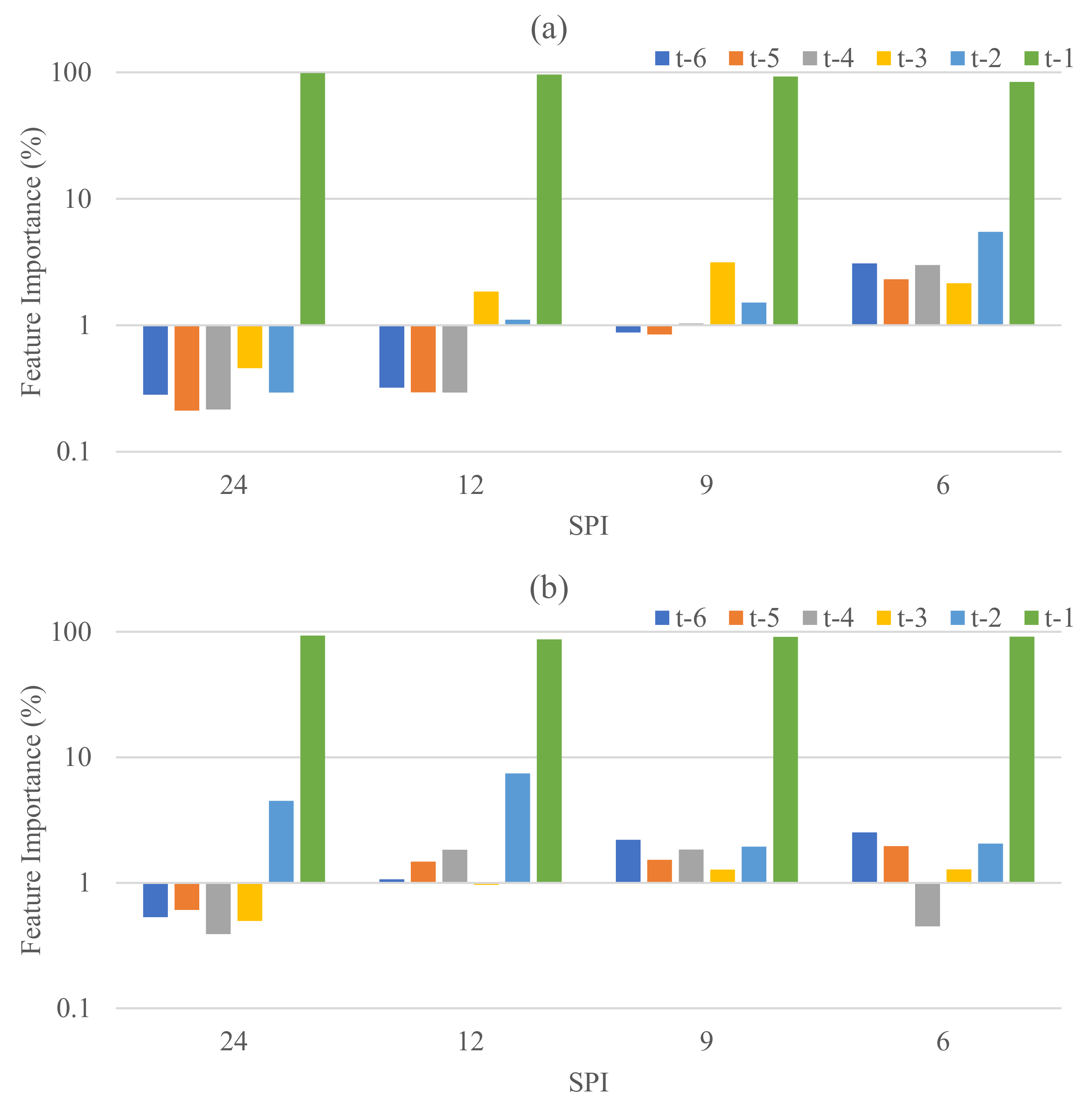
The XGBoost feature importance analysis was carried out across all stations to predict the 6-, 9-, 12-, and 24-month SPIs with a lag time of 6 months, specifically defined as t−1 (one period prior) to t−6 (six periods prior) relative to the current SPI. As illustrated in Figure 5, the feature importance analysis revealed that SPI values from the previous day emerged as the most crucial feature, with importance scores exceeding 90%. Conversely, SPI values from preceding days exhibited lower importance scores, generally below 10% and frequently below 2%, depending on different scenarios, suggesting the potential of considering the SPI values from the previous day in predicting future SPI values. This observation aligned with expectations, akin to the Pearson correlation test, indicating the high impact of the SPI values from t−1. Also, it is recommended that future investigations profoundly explore the relationship between historical SPI values, to enhance comprehension of their influence. Based on the results of the feature importance analysis, a feature with a low importance value may still contribute to the overall model performance. Therefore, while these findings highlight the importance of the SPI values from the previous day, they do not dismiss the inevitable impact of the SPI values from previous months (rather than t−1) on the outcome. Thus, conclusions should not be based solely on this analysis, and further exploration is warranted.

3.3. Results of Confidence Percentages for Machine Learning Models

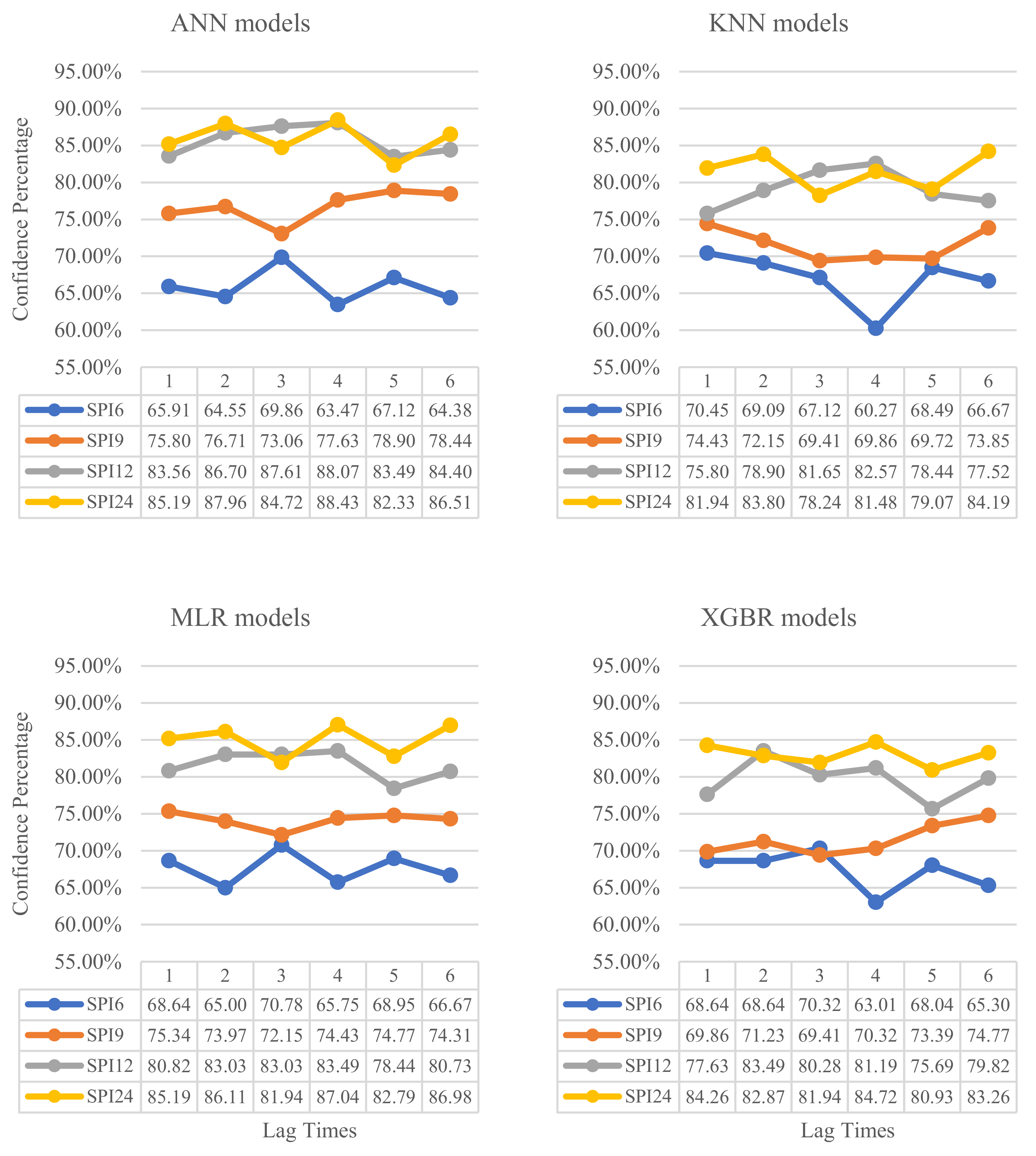
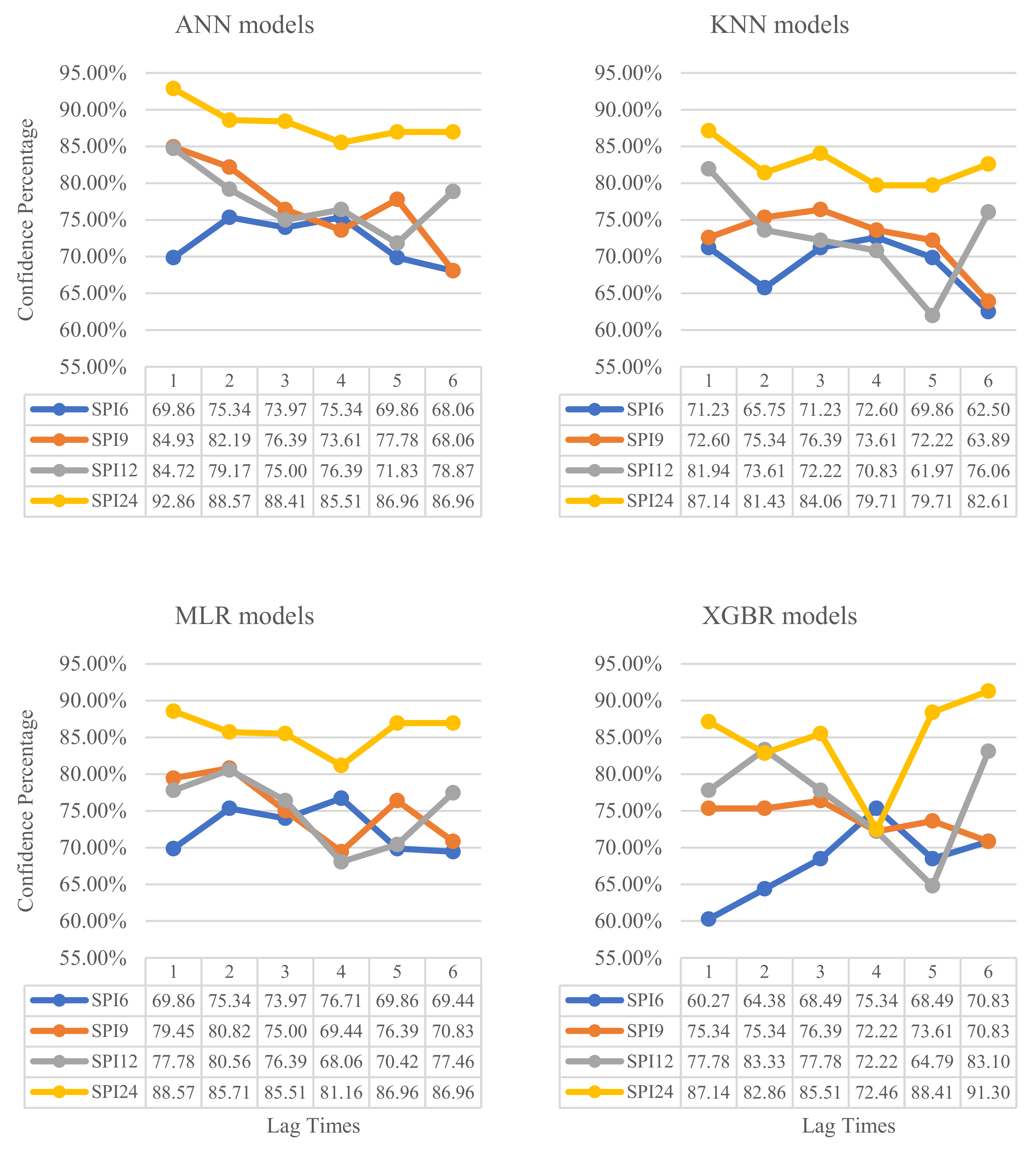
Figure 6 and Figure 7 illustrate the results of CPs for each scenario for Shiraz and Tridolino stations, respectively. Each figure contains plots corresponding to the four ML models used in this study. In each plot, the x-axis denotes the lag times, while the y-axis shows CP. Additionally, each line in Figure 6 and Figure 7 represents the CP results for a specific SPI duration. Overall, the CP results displayed a trend consistent with the findings of the metric results reported in Section 3.1.
According to Figure 6, for the 6-month SPI, when comparisons were made based on lag time, the lowest CP was 60.27% for the KNN model with a lag time of 4, while the highest CP was 70.78% for the MLR model with a lag time of 3. In general, lag times of 3 were associated with the highest CP. For the 9-month SPI, the lowest and highest CP values were 69.41% for the KNN model with a lag time of 3 and 78.9% for the ANN model with a lag time of 5, respectively. While the CP results did not demonstrate clear differences for the 6-month SPI, the model performance was more stable across different lag times. To be more specific, the ANN model outperformed others, followed by the MLR model. For the 12-month SPI, the lowest and highest CP values were 75.69% for the XGBR model with a lag time of 5 and 88.07% for the ANN model with a lag time of 4, respectively. The ML models showed a relatively stable performance across different lag times for the 12-month SPI, with lag times ranging from 2 to 4 appearing as suitable options. As indicated in Figure 6, it was also evident that the ANN model overall outperformed other models for the 12-month SPI. For the 24-month SPI, the lowest and highest CP values were 78.24% for the KNN model with a lag time of 3 and 88.43% for the ANN model with a lag time of 4, respectively. Unlike the results for the other SPIs, no clear conclusions could be drawn regarding the best-case scenario for the 24-month SPI, even though lag times of 3 and 5 were associated with weaker performances. Finally, the ANN and MLR models again produced the best CP values.
The CP results obtained for Tridolino station demonstrated a general trend similar to those observed at Shiraz station. As shown in Figure 7, for the 6-month SPI, the lowest CP was 60.27% for the XGBR model with a lag time of 1, while the highest CP was 76.71% for the MLR model with a lag time of 4. In general, a lag time of 4 exhibited the highest CP for Shiraz station. For the 9-month SPI, the lowest and highest CP values were 63.89% for the KNN model with a lag time of 6 and 84.93% for the ANN model with a lag time of 1, respectively. No strong conclusion could be made regarding the best-performing model for the 9-month SPI. Similarly, a definitive choice of the optimal lag time remains unclear. For the 12-month SPI, the lowest CP was 61.97% for the KNN model with a lag time of 5, and the highest CP was 84.72% for the ANN model with a lag time of 1. Likewise, no recommendation can be made about the best combination of ML models or lag times for SPI analysis. Unlike Shiraz station, the ML performances for the 9-month SPI were better than that for the 6-month SPI, while the CP results for the 12-month SPI did not show any improvement. However, the 24-month SPI showed a significant improvement compared with the shorter SPI durations. For the 24-month SPI, the lowest and highest CP values were 72.46% for the XGBR model with a lag time of 4 and 92.86% for the ANN model with a lag time of 1, respectively. No clear conclusions could be drawn regarding the best model or lag time for the 24-month SPI, even though a lag time of 4 was associated with a weaker performance, particularly for the XGBR model.
In summary, the CP results, similar to the statistical metrics, improved as the SPI duration increased. Nevertheless, the performances of the ML models for the 12-month SPI and 24-month SPI were relatively close, with some scenarios with lag times of 3 and 5 suggesting higher confidence in the 12-month SPI compared with the 24-month SPI.

3.4. Comparison between Two Different Stations

Adaptation measures are necessary not only to cope with the changes already underway but also to minimize negative impacts on vulnerable communities and ecosystems. For drought mitigation and preparedness, drought analysis based on SPI helps in water resource management, agriculture, and decision making. To be more specific, SPI focuses solely on precipitation and does not consider other factors such as temperature or evaporation, which can also influence drought conditions. Since this study conducted an SPI-based drought analysis, other factors that may have an influence on this natural hazard were neglected, which represents a limitation of the present study. Therefore, it is suggested that further studies should use SPI in conjunction with other indices and information sources to provide a comprehensive understanding of drought patterns and impacts.
Across the various modeling scenarios considered in this study, the optimal ML model varied based on influencing factors such as station, lag time, or return period when calculating the drought index. Furthermore, additional aspects, such as computational efficiency, interpretability, ease of implementation, and requirements inherent to the problem under consideration, should be considered for selecting the most suitable ML model for estimating SPI. For example, among the ML models utilized in this study, ANN and XGBR generally performed adequately with higher accuracy compared with the others, specifically for capturing the complex and nonlinear relationships of data from different stations and with multiple lag times. Moreover, ANN requires a relatively high level of computational resources, while XGBR is balanced in both accuracy and efficiency. KNN, as simple and straightforward as it is, may pose a problem when dealing with large datasets with high dimensionality and cause overfitting. On the other hand, MLR, being a basic linear model, has more interpretability but less flexibility in capturing nonlinear patterns, and consequently, it performs less adequately in more complex cases. Therefore, the choice of ML models depends on the trade-offs between complexity, interpretability, and computational efficiency.
Based on the results shown in Figure 3 and Figure 4, the performances of ML models for long-term SPI timescales, such as the 24-month SPI, surpassed that for shorter-term SPIs, like the 6-month SPI, similar to previous studies [4,5,6,8,12,13,17,22,23]. Furthermore, the overall performance of the ML models exhibited minimal variation, mirroring outcomes observed in previous research [14]. Furthermore, ANN obtained different optimal lag times for each SPI for Shiraz station (lag times of 6, 6, 4, and 2 for SPIs of 6, 9, 12, and 24 months, respectively) in terms of the four performance evaluation criteria. Nevertheless, no specific optimum lag time could be reported for SPI values for Tridolino station when considering the four indices (i.e., RMSE, MAE, NSE, and R2). Therefore, there was a distinctive difference between the results obtained for Shiraz station (Iran) and those achieved for Tridolino station (Italy).
According to the CP results, the CP values for both stations improved as the SPI duration increased. Nonetheless, for Shiraz station, the CP values for the 12-month SPI and 24-month SPI were quite close, while for Tridolino station, the 9-month SPI and 12-month SPI showed similar results, with the 24-month SPI yielding primarily higher CP values. Overall, all the ML models demonstrated high percentages of confidence in their estimations, with none of the CP values falling below 60% and some CP values being above 90% in certain scenarios.
The results obtained in the current study indicated the satisfactory performances of the ML models for both stations. Given the diverse climatic conditions and geographical separation of these stations, the ML models can be utilized effectively for SPI-based drought analysis in these regions. Similarly, Adikari et al. [21] explored various stations in Australia and Cambodia; however, their study did not investigate different lag times and timeframes of SPI. Furthermore, their models, namely a Convolutional Neural Network, LSTM, and wavelet decomposition functions combined with the Adaptive Neuro-Fuzzy Inference System, shared a common conceptual basis to some extent, whereas the current study offers a broader coverage of the mentioned limitations.
In summary, ANN outperformed the other ML models used in this study for Shiraz station, whereas no ML modes outperformed the others in terms of the four metrics for estimating SPI values for Tridolino station. Finally, KNN resulted in SPI estimations with the lowest precision for many cases considered for both stations in this study, similar to the results of a previous study [14]. This study, akin to various studies available in the literature [6,9,10,12,14,17,22,24,25], highlights the need to consider different combinations of lag times as input, as no firm conclusion on the optimal number of lag times can be made. The focus of this study was on comparing performances of ML models rather than an in-depth assessment of agricultural or hydrological drought conditions in the study areas. Future studies can utilize the SPI values predicted by our models for further drought assessments. Indeed, using only two stations limits the generalizability of an assessment of drought conditions. However, this study provides valuable insights into the performance of different ML models across two climatically distinct regions, which can serve as a basis for future research using broader datasets.

4. Conclusions

This study provides valuable insights into the effectiveness of ML-based drought prediction methodologies and highlights the importance of tailoring ML models to specific geographical contexts for enhanced applicability and accuracy. It provides a comprehensive analysis of drought conditions in two distinct stations with two different climates, Shiraz in Iran and Tridolino in Italy, using ML models to forecast SPI values. By examining different scenarios and considering different lag times, this study not only contributes to our understanding of predicting drought indicators but also highlights the importance of comparative assessments of ML approaches across diverse geographical locations.
The results showed that the performance of ML models varied based on the station, lag time, and SPI duration. Specifically, the ANN model exhibited robust estimations for SPI values at Shiraz station, while no single ML model consistently outperformed the others for Tridolino station. This variability underscores the importance of not only tailoring ML approaches to specific contexts but also considering multiple factors when selecting the most suitable model. Furthermore, CP values were computed for each ML model to assess the capability and reliability of the predictions made by the ML models. Analysis of CP values revealed that higher SPI durations generally led to better estimations for both stations. Overall, all the ML models demonstrated a high level of confidence, with CP values no lower than 60% and up to 90% for some cases. Additionally, similar to the metric results, the ANN models generally outperformed the other ML models in terms of CP performances for Shiraz station, while no single ML model consistently outperformed the others for Tridolino station.
Moreover, this study highlights the need for further research to explore the synergies between SPI and other drought indices or environmental variables to enhance the accuracy and comprehensiveness of drought prediction models. Future studies can explore incorporating other drought indices, such as the Palmer Drought Severity Index or the Standardized Precipitation Evapotranspiration Index, to provide a more nuanced understanding of drought dynamics and impacts.
Additionally, while this study focused on SPI-based drought analysis, future studies could also investigate the integration of remote sensing data and climate model outputs to improve the spatial and temporal resolutions of drought predictions.
Overall, the satisfactory performance of the ML models across both the Iranian and Italian stations suggests the potential applicability of these approaches in diverse climatic conditions. However, continued research and refinement of ML techniques are necessary to improve the accuracy and reliability of drought prediction models, ultimately supporting effective water resource management and climate change adaptation efforts worldwide.

Supplementary Materials

The following supporting information can be downloaded at: https://www.mdpi.com/article/10.3390/hydrology11100163/s1, Table S1: Metric results for Shiraz station; Table S2: Metric results for Tridolino station.

Author Contributions

All authors contributed to the study conception and design. Material preparation and data collection were performed by M.N., F.G., G.E.T. and S.H.A. The analysis was conducted by R.P. and M.N. The first draft of the manuscript was written by R.P., M.N., F.G. and G.E.T. and all authors commented on previous versions of the manuscript. All authors have read and agreed to the published version of the manuscript.

Funding

The authors declare that no funds, grants, or other support were received during the preparation of this manuscript.

Data Availability Statement

The data used in this study can be supplied by the corresponding author upon request.

Conflicts of Interest

The authors have no relevant financial or non-financial interests to disclose.

References

  1. Cheng, M.; McCarl, B.; Fei, C. Climate change and livestock production: A literature review. Atmosphere 2022, 13, 140. [Google Scholar] [CrossRef]
  2. Bouaziz, M.; Medhioub, E.; Csaplovisc, E. A machine learning model for drought tracking and forecasting using remote precipitation data and a standardized precipitation index from arid regions. J. Arid Environ. 2021, 189, 104478. [Google Scholar] [CrossRef]
  3. Shokoohi, A.; Morovati, R. Basinwide comparison of RDI and SPI within an IWRM framework. Water Resour. Manag. 2015, 29, 2011–2026. [Google Scholar] [CrossRef]
  4. Hosseini-Moghari, S.M.; Araghinejad, S. Monthly and seasonal drought forecasting using statistical neural networks. Environ. Earth Sci. 2015, 74, 397–412. [Google Scholar] [CrossRef]
  5. Docheshmeh Gorgij, A.; Alizamir, M.; Kisi, O.; Elshafie, A. Drought modelling by standard precipitation index (SPI) in a semi-arid climate using deep learning method: Long short-term memory. Neural Comput. Appl. 2022, 34, 2425–2442. [Google Scholar] [CrossRef]
  6. Lotfirad, M.; Esmaeili-Gisavandani, H.; Adib, A. Drought monitoring and prediction using SPI, SPEI, and random forest model in various climates of Iran. J. Water Clim. Change 2022, 13, 383–406. [Google Scholar] [CrossRef]
  7. Piri, J.; Abdolahipour, M.; Keshtegar, B. Advanced machine learning model for prediction of drought indices using hybrid SVR-RSM. Water Resour. Manag. 2023, 37, 683–712. [Google Scholar] [CrossRef]
  8. Shakeri, R.; Amini, H.; Fakheri, F.; Ketabchi, H. Assessment of drought conditions and prediction by machine learning algorithms using Standardized Precipitation Index and Standardized Water-Level Index (case study: Yazd province, Iran). Environ. Sci. Pollut. Res. 2023, 30, 101744–101760. [Google Scholar] [CrossRef]
  9. Elbeltagi, A.; Kumar, M.; Kushwaha, N.; Pande, C.B.; Ditthakit, P.; Vishwakarma, D.K.; Subeesh, A. Drought indicator analysis and forecasting using data driven models: Case study in Jaisalmer, India. Stoch. Environ. Res. Risk Assess. 2023, 37, 113–131. [Google Scholar] [CrossRef]
  10. Elbeltagi, A.; Pande, C.B.; Kumar, M.; Tolche, A.D.; Singh, S.K.; Kumar, A.; Vishwakarma, D.K. Prediction of meteorological drought and standardized precipitation index based on the random forest (RF), random tree (RT), and Gaussian process regression (GPR) models. Environ. Sci. Pollut. Res. 2023, 30, 43183–43202. [Google Scholar] [CrossRef]
  11. Coşkun, Ö.; Citakoglu, H. Prediction of the standardized precipitation index based on the long short-term memory and empirical mode decomposition-extreme learning machine models: The Case of Sakarya, Türkiye. Phys. Chem. Earth Parts A/B/C 2023, 131, 103418. [Google Scholar] [CrossRef]
  12. Adnan, R.M.; Dai, H.-L.; Kuriqi, A.; Kisi, O.; Zounemat-Kermani, M. Improving drought modeling based on new heuristic machine learning methods. Ain Shams Eng. J. 2023, 14, 102168. [Google Scholar] [CrossRef]
  13. Saha, S.; Kundu, B.; Paul, G.C.; Pradhan, B. Proposing an ensemble machine learning based drought vulnerability index using M5P, dagging, random sub-space and rotation forest models. Stoch. Environ. Res. Risk Assess. 2023, 37, 2513–2540. [Google Scholar] [CrossRef]
  14. Niazkar, M.; Piraei, R.; Eryılmaz Türkkan, G.; Hırca, T.; Gangi, F.; Afzali, S.H. Drought analysis using innovative trend analysis and machine learning models for Eastern Black Sea Basin. Theor. Appl. Climatol. 2024, 155, 1605–1624. [Google Scholar] [CrossRef]
  15. Belayneh, A.; Adamowski, J. Standard precipitation index drought forecasting using neural networks, wavelet neural networks, and support vector regression. Appl. Comput. Intell. Soft Comput. 2012, 2012, 794061. [Google Scholar] [CrossRef]
  16. Belayneh, A.; Adamowski, J.; Khalil, B.; Ozga-Zielinski, B. Long-term SPI drought forecasting in the Awash River Basin in Ethiopia using wavelet neural network and wavelet support vector regression models. J. Hydrol. 2014, 508, 418–429. [Google Scholar] [CrossRef]
  17. Belayneh, A.; Adamowski, J.; Khalil, B.; Quilty, J. Coupling machine learning methods with wavelet transforms and the bootstrap and boosting ensemble approaches for drought prediction. Atmos. Res. 2016, 172, 37–47. [Google Scholar] [CrossRef]
  18. Maca, P.; Pech, P. Forecasting SPEI and SPI drought indices using the integrated artificial neural networks. Comput. Intell. Neurosci. 2016, 2016, 3868519. [Google Scholar] [CrossRef]
  19. El Ibrahimi, A.; Baali, A. Application of Several Artificial Intelligence Models for Forecasting Meteorological Drought Using the Standardized Precipitation Index in the Saïss Plain (Northern Morocco). Int. J. Intell. Eng. Syst. 2018, 11, 267–275. [Google Scholar] [CrossRef]
  20. Khan, M.M.H.; Muhammad, N.S.; El-Shafie, A. Wavelet based hybrid ANN-ARIMA models for meteorological drought forecasting. J. Hydrol. 2020, 590, 125380. [Google Scholar] [CrossRef]
  21. Adikari, K.E.; Shrestha, S.; Ratnayake, D.T.; Budhathoki, A.; Mohanasundaram, S.; Dailey, M.N. Evaluation of artificial intelligence models for flood and drought forecasting in arid and tropical regions. Environ. Model. Softw. 2021, 144, 105136. [Google Scholar] [CrossRef]
  22. Malik, A.; Kumar, A.; Rai, P.; Kuriqi, A. Prediction of multi-scalar standardized precipitation index by using artificial intelligence and regression models. Climate 2021, 9, 28. [Google Scholar] [CrossRef]
  23. Taylan, E.D.; Terzi, Ö.; Baykal, T. Hybrid wavelet–artificial intelligence models in meteorological drought estimation. J. Earth Syst. Sci. 2021, 130, 38. [Google Scholar] [CrossRef]
  24. Pande, C.B.; Costache, R.; Sammen, S.S.; Noor, R.; Elbeltagi, A. Combination of data-driven models and best subset regression for predicting the standardized precipitation index (SPI) at the Upper Godavari Basin in India. Theor. Appl. Climatol. 2023, 152, 535–558. [Google Scholar] [CrossRef]
  25. Ham, Y.-S.; Sonu, K.-B.; Paek, U.-S.; Om, K.-C.; Jong, S.-I.; Jo, K.-R. Comparison of LSTM network, neural network and support vector regression coupled with wavelet decomposition for drought forecasting in the western area of the DPRK. Nat. Hazards 2023, 116, 2619–2643. [Google Scholar] [CrossRef]
  26. Hukkeri, G.S.; Naganna, S.R.; Pruthviraja, D.; Bhat, N.; Goudar, R. Drought forecasting: Application of ensemble and advanced machine learning approaches. IEEE Access 2023, 11, 141375–141393. [Google Scholar] [CrossRef]
  27. Lalika, C.; Mujahid, A.U.H.; James, M.; Lalika, M.C. Machine learning algorithms for the prediction of drought conditions in the Wami River sub-catchment, Tanzania. J. Hydrol. Reg. Stud. 2024, 53, 101794. [Google Scholar] [CrossRef]
  28. Mohammed, S.; Arshad, S.; Alsilibe, F.; Moazzam, M.F.U.; Bashir, B.; Prodhan, F.A.; Alsalman, A.; Vad, A.; Ratonyi, T.; Harsányi, E. Utilizing machine learning and CMIP6 projections for short-term agricultural drought monitoring in central Europe (1900–2100). J. Hydrol. 2024, 633, 130968. [Google Scholar] [CrossRef]
  29. European Commission. Standardized Precipitation Index (SPI), Copernicus European Drought Observatory (EDO), EDO Indicator Factsheet—Standardized Precipitation Index (SPI); European Commission: Brussels, Belgium, 2022. [Google Scholar]
  30. Guttman, N.B. Accepting the standardized precipitation index: A calculation algorithm 1. JAWRA J. Am. Water Resour. Assoc. 1999, 35, 311–322. [Google Scholar] [CrossRef]
  31. Piraei, R.; Afzali, S.H.; Niazkar, M. Assessment of XGBoost to Estimate Total Sediment Loads in Rivers. Water Resour. Manag. 2023, 37, 5289–5306. [Google Scholar] [CrossRef]
  32. Chen, T.; Guestrin, C. Xgboost: A scalable tree boosting system. In Proceedings of the 22nd ACM Sigkdd International Conference on Knowledge Discovery and Data Mining, San Francisco, CA, USA, 13–17 August 2016. [Google Scholar]
  33. Chollet, F. Keras: The Python Deep Learning Library; Astrophysics Source Code Library: Houghton, MI, USA, 2018; p. ascl: 1806.022. [Google Scholar]
  34. Pedregosa, F.; Varoquaux, G.; Gramfort, A.; Michel, V.; Thirion, B.; Grisel, O.; Blondel, M.; Prettenhofer, P.; Weiss, R.; Dubourg, V.; et al. Scikit-learn: Machine learning in Python. J. Mach. Learn. Res. 2011, 12, 2825–2830. [Google Scholar]
  35. Dikshit, A.; Pradhan, B.; Santosh, M. Artificial neural networks in drought prediction in the 21st century—A scientometric analysis. Appl. Soft Comput. 2022, 114, 108080. [Google Scholar] [CrossRef]
  36. Zhang, R.; Chen, Z.-Y.; Xu, L.-J.; Ou, C.-Q. Meteorological drought forecasting based on a statistical model with machine learning techniques in Shaanxi province, China. Sci. Total Environ. 2019, 665, 338–346. [Google Scholar] [CrossRef] [PubMed]
  37. Niazkar, M.; Menapace, A.; Brentan, B.; Piraei, R.; Jimenez, D.; Dhawan, P.; Righetti, M. Applications of XGBoost in water resources engineering: A systematic literature review (Dec 2018–May 2023). Environ. Model. Softw. 2024, 174, 105971. [Google Scholar] [CrossRef]
  38. Ali, S.; Khorrami, B.; Jehanzaib, M.; Tariq, A.; Ajmal, M.; Arshad, A.; Shafeeque, M.; Dilawar, A.; Basit, I.; Zhang, L.; et al. Spatial Downscaling of GRACE Data Based on XGBoost Model for Improved Understanding of Hydrological Droughts in the Indus Basin Irrigation System (IBIS). Remote Sens. 2023, 15, 873. [Google Scholar] [CrossRef]
  39. Altunkaynak, A.; Jalilzadnezamabad, A. Extended lead time accurate forecasting of palmer drought severity index using hybrid wavelet-fuzzy and machine learning techniques. J. Hydrol. 2021, 601, 126619. [Google Scholar] [CrossRef]
  40. Raja, A.; Gopikrishnan, T. Drought prediction and validation for desert region using machine learning methods. Int. J. Adv. Comput. Sci. Appl. 2022, 13. [Google Scholar] [CrossRef]
  41. Fadaei-Kermani, E.; Barani, G.; Ghaeini-Hessaroeyeh, M. Drought monitoring and prediction using K-nearest neighbor algorithm. J. AI Data Min. 2017, 5, 319–325. [Google Scholar]
  42. Niazkar, M.; Piraei, R.; Zakwan, M. Application of Machine Learning Models for Short-term Drought Analysis Based on Streamflow Drought Index. Water Resour. Manag. 2024, 1–18. [Google Scholar] [CrossRef]
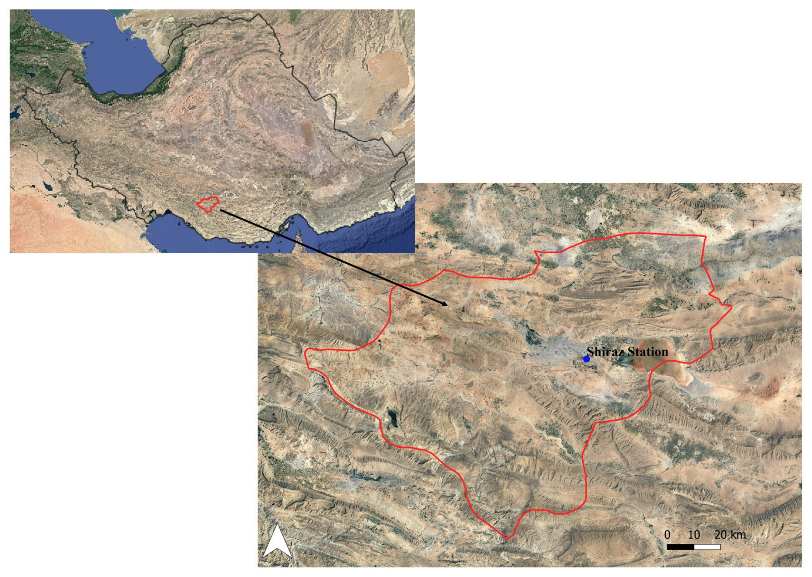
Figure 1. Location map of Shiraz weather station in Iran (blue dot), in the Shiraz watershed (red line).
Hydrology 11 00163 g001
Figure 2. Location map of Mantova Tridolino pluviometric station (blue dot), in the Lombardy region (red line).
Hydrology 11 00163 g002
Figure 3. Heatmap of the metric results for Shiraz station for all ML models utilized in this study.
Hydrology 11 00163 g003
Figure 4. Heatmap of the metric results for Tridolino station for all ML models utilized in this study.
Hydrology 11 00163 g004
Figure 5. Feature importance analysis results for (a) Shiraz station and (b) Tridolino station.
Hydrology 11 00163 g005
Figure 6. CP results obtained for Shiraz station for different machine learning models and time lags.
Hydrology 11 00163 g006
Figure 7. CP results obtained for Tridolino station for different machine learning models and time lags.
Hydrology 11 00163 g007
Table 1. Overview of ML models and lead times in previous studies and this study.
StudyYearStationsSPI MonthsML Models Used for ComparisonBest Resulting Model
Belayneh and Adamowski [15]201233, 12ANN, SVR, and WNWN
Belayneh et al. [16]20141212, 24ARIMA, ANN, SVR, WA-ANN, and WA-SVRWA-ANN
Hosseini-Moghari and Araghinejad [4]201513, 6, 9, 12, 24RMSMLP, DMSMLP, RMSRBF, DMSRBF, RMSGRNN, and DMSGRNNRMSRBF and RMSGRNN, for smaller time scales, DMSRBF and DMSGRNN for larger ones.
Belayneh et al. [17]201633, 12, 24BANN, BSVR, WA-ANN, WA-SVR, BS-ANN, BS-SVR, WBS-ANN, and WBS-SVRWBS-ANN and WBS-SVR
Maca and Pech [18]201621sANN and hANNhANN
El Ibrahimi and Baali [19]201823, 12ANFIS, ANN, and SVRANFIS
Khan et al. [20]202031WN, ARIMA, ANN, and W-2AW-2A
Adikari et al. [21]2021131CNN, LSTM, and WANFISWANFIS
Malik et al. [22]202171, 3, 6, 9, 12, 24ANN, CANFIS, and MLRCANFIS and MLR
Docheshmeh Gorgij et al. [5]202143, 6, 9, 12LSTM, MARS, ET, and VARLSTM
Taylan et al. [23]202133, 6, 9, 12ANFIS, SVM, ANN, WA-ANFIS, WA-ANN, and WA-SVRWA-ANFIS for 12-month SPI and WA-SVR for other SPIs
Lotfirad et al. [6]202261, 3, 6, 9, 12, 24, 48RFRF
Piri et al. [7]2022111ANN, SVR, SVR-PSO, and SVR-RSMSVR-RSM
Shakeri et al. [8]202313, 6, 12, 24MLR, KNN, GB, DT, XGBR, RF, and ANNANN
Pande et al. [24]202333, 6, 12AR, RSS, M5P, and BTM5P and BT
Elbeltagi et al. [9]202313, 6, 12RSS, RSS-M5P, RSS-RF, and RSS-RTRSS-M5P
Elbeltagi et al. [10]202326, 12RF, RT, and GPR-PUK kernelRF
Ham et al. [25]202366, 12WLSTMN, WA-ANN, and WA-SVRWLSTMN
Coşkun and Citakoglu [11]202311, 3, 6LSTM, EMD, and ELMLSTM
Adnan et al. [12]202333, 6, 9, 12OP-ELM, DENFIS, and MARSDENFIS
Saha et al. [13]202313, 6, 12, 24M5P, M5P-Dagging, M5P-RSS, and M5P-RTFM5P-RFT
Niazkar et al. [14] 202386, 9, 12, 24ANN, MLR, KNN, XGBRANN, MLR, and XGBR
Hukkeri et al. [26]2023126ANN, MARS, GB, CBRMARS and GB
Lalika et al. [27]202456, 9LSTM, MARS, SVR, ELM, M5PLSTM
Mohammed et al. [28] 202433BT, RF, DT, M5PRF
Abbreviations: ANFIS: Adaptive Neuro-Fuzzy Inference System; AR: Additive Regression; ARIMA: Autoregressive Integrated Moving Average; BANN: Bootstrap ANN; BS-ANN: Boosting Ensemble with ANN; BS-SVR: Boosting Ensemble with SVR; BSVR: Bootstrap SVR; BT: Bagging Tree; CANFIS: Co-Active Neuro-Fuzzy Inference System; CBR: CatBoost Regression; CNN: Convolutional Neural Network; DMSGRNN: Direct Multi-Step Generalized Regression Neural Network; DMSMLP: Direct Multi-Step Multi-Layer Perceptron; DMSRBF: Direct Multi-Step Radial Basis Function; DT: decision tree; GB: gradient boosting; GPR-PUK kernel: Gaussian process regression; hANN: integrated neural network; RMSGRNN: Recursive Multi-Step Generalized Regression Neural Network; RMSMLP: Recursive Multi-Step Multi-Layer Perceptron; RMSRBF: Recursive Multi-Step Radial Basis Function; RSS-M5P: Hybridization of RSS with M5P; RSS-RF: Hybridization of RSS with RF; RSS-RT: Hybridization of RSS with RT; sANN: feedforward multilayer perceptron; SVR-PSO: SVR with Particle Swarm Optimization; SVR-RSM: SVR with Response Surface Method; VR: Voting Regressor; W-2A: Hybrid ensemble of WN, ANN, and ARIMA; WA-ANN: ANN coupled with wavelet transform; WA-ANFIS: ANFIS coupled with wavelet transform; WANFIS: wavelet decomposition functions combined with ANFIS; WA-SVR: SVR coupled with wavelet transform; WBS-ANN: wavelet boosting with ANN; WBS-SVR: wavelet boosting with SVR; WLSTMN: wavelet long short-term memory network; WN: Wavelet Neural Network.
Table 2. Statistical properties of precipitation (P) and SPI values with different time scales for Shiraz and Tridolino stations.
Statistical PropertyShiraz StationTridolino Station
P (mm)SPIP (mm)SPI
691224691224
Minimum0−2.51−2.51−2.51−2.500−2.10−2.10−2.10−2.08
Average26.810.020.0010.0014 × 10−440.07−4 × 10⁻¹⁶−7 × 10⁻¹⁶−9 × 10⁻¹⁶−2 × 10⁻¹⁶
Maximum3302.512.512.512.50159.362.102.102.102.08
Skewness2.400.06−0.0010.001−5 × 10−41.003 × 10−161 × 10−161 × 10−153 × 10−16
Standard deviation43.760.970.990.990.9929.510.970.970.970.97
Table 3. Brief description of key hyperparameters tuned for each machine learning model.
ModelHyperparameterDescriptionRange
ANNactivationThe activation function introduces nonlinearity to models.‘tanh’, ‘relu’, ‘sigmoid’, and ‘linear’
optimizerOptimizer algorithm determines optimal weights for the model.‘sgd’, ‘rmsprop’, ‘adadelta’, and ‘adam’
lossThe loss function measures the model performance.‘mae’, ‘mse’, or other defined metrics in ‘keras’ library
KNNpPower parameter for the Minkowski metric.float
n_neighborsNumber of neighbors.positive integer
weightsWeight function is used in prediction.‘uniform’, ‘distance’, callable or none
algorithmAlgorithm is used to compute the nearest neighbors.‘auto’, ‘ball_tree’, ‘kd_tree’, and ‘brute’
XGBRn_estimatorsNumber of trees.positive integer
max_depthMaximum depth allowed for each tree.positive integer or none
learning_rateStep size shrinkage is used to prevent overfitting (eta).[0, 1]
reg_alphaL1 weight regularization term.[0, ∞]
reg_lambdaL2 weight regularization term.[0, ∞]
min_split_lossMinimum loss reduction required to make a further partition on a leaf node of the tree (gamma).[0, ∞]
min_child_weightMinimum summation of the instance weight needed in a child node.[0, ∞]
Disclaimer/Publisher’s Note: The statements, opinions and data contained in all publications are solely those of the individual author(s) and contributor(s) and not of MDPI and/or the editor(s). MDPI and/or the editor(s) disclaim responsibility for any injury to people or property resulting from any ideas, methods, instructions or products referred to in the content.