Article

Assessing the Impact of Rainfall Inputs on Short-Term Flood Simulation with Cell2Flood: A Case Study of the Waryong Reservoir Basin

1
Department of Agricultural Engineering, Gyeongsang National University, Jinju 52828, Republic of Korea
2
Department of Agricultural Engineering, Chungnam National University, Daejeon 34134, Republic of Korea
3
School of Social Safety and Systems Engineering, Institute of Agricultural Environmental Science, Hankyong National University, Anseong 17579, Republic of Korea
4
Department of Agricultural Engineering, Institute of Agricultural and Life Science, Gyeongsang National University, Jinju 52828, Republic of Korea
*
Author to whom correspondence should be addressed.
Hydrology 2024, 11(10), 162; https://doi.org/10.3390/hydrology11100162
Submission received: 12 September 2024 / Revised: 28 September 2024 / Accepted: 1 October 2024 / Published: 2 October 2024

Abstract

:
This study explored the impacts of various rainfall input types on short-term runoff simulations using the Cell2Flood model in the Waryong Reservoir Basin, South Korea. Six types of rainfall data were assessed: on-site gauge measurements, spatially interpolated data from 39 Automated Synoptic Observing System (ASOS) and 117 Automatic Weather System (AWS) stations using inverse distance weighting (IDW), and Hybrid Surface Rainfall (HSR) data from the Korea Meteorological Administration. The choice of rainfall input significantly affected model accuracy across the three rainfall events. The point-gauged ASOS (P-ASOS) data demonstrated the highest reliability in capturing the observed rainfall patterns, with Pearson’s r values of up to 0.84, whereas the radar-derived HSR data had the lowest correlations (Pearson’s r below 0.2), highlighting substantial discrepancies. For runoff simulation, the P-ASOS and ASOS-AWS combined interpolated dataset (R-AWS) achieved relatively accurate predictions, with P-ASOS and R-AWS exhibiting Normalized Peak Error (NPE) values of approximately 0.03 and Peak Time Error (PTE) within 20 min. In contrast, the HSR data produced large errors, with NPE up to 4.66 and PTE deviations exceeding 200 min, indicating poor temporal accuracy. Although input-specific calibration improved performance, significant errors persisted because of the inherent uncertainty of rainfall data. These findings underscore the importance of selecting and calibrating appropriate rainfall inputs to enhance the reliability of short-term flood modeling, particularly in ungauged and data-sparse basins.

1. Introduction

Climate change has intensified the frequency and severity of water-related disasters such as typhoons, flash floods, and heavy rainfall, causing substantial damage. In response, flood prediction and mitigation technologies have rapidly evolved, with rainfall–runoff models being the principal components of these efforts. Various rainfall–runoff models have been developed and utilized over the years. However, the choice of rainfall input data is the most crucial factor in determining the accuracy and reliability of the simulation outcomes regardless of the model. Accurate rainfall data are essential for predicting reservoir inflows, scheduling water releases, and maintaining sufficient storage capacity to mitigate flood risks while ensuring a stable water supply for irrigation. Inaccurate rainfall data can lead to premature or delayed water release, compromising dam safety and increasing downstream flood risk.
Typically, rainfall data are collected from ground-based meteorological stations. However, in rural and forested regions, the low density and spatial variability of rainfall observation stations render securing reliable rainfall data necessary for accurate flood forecasting and modeling challenging. Rainfall data used in flood modeling are generally divided into three categories: gauge measurements, spatially interpolated data, and radar-derived data. Gauge measurements, the most traditional and widely implemented method, provide high temporal resolution but are limited in spatial coverage, particularly in regions with complex topography. This limitation can result in an insufficient representation of rainfall variability. Spatially interpolated data offer improved spatial representation by integrating observations from multiple gauges; however, they inherently involve uncertainties owing to the interpolation process. Radar-derived rainfall data, which have recently been increasingly used, provide real-time coverage over extensive areas but are often criticized for their lower spatial resolution, particularly in small catchments, and discrepancies with in situ measurements remain problematic [1].
The Korea Meteorological Administration (KMA) manages a network of 105 Automated Synoptic Observing System (ASOS) and 554 Automated Weather System (AWS) stations in South Korea. ASOS stations are primarily designed for extensive meteorological observations and international data sharing. In contrast, AWS stations are strategically located in remote and hard-to-reach areas such as mountainous regions and islands to provide real-time monitoring of localized severe weather conditions. Both the ASOS and AWS capture meteorological data at various temporal resolutions, from minutes to years. The ASOS, with its extensive history of data collection dating back to 1904, provides a rich dataset for climate studies. In contrast, the AWS stations, which were first installed in 1997, have a shorter data history. This discrepancy in data accumulation periods presents challenges in maintaining statistical consistency in meteorological and hydrological research. Despite the extensive coverage these networks provide, obtaining reliable and dense rainfall data remains a significant challenge, particularly in sparsely populated and remote regions [2]. Efforts have been made to mitigate the lack of consistent and long-term hydrometeorological data in areas with sparse hydrological records and limited on-site observation systems, such as agricultural reservoir catchments [3]. However, practical constraints often result in sparse observation networks. This is particularly true for rural regions, where the potential for human and economic losses is considered lower, leading to these areas being deprioritized in the allocation of observational resources [4].
Although rainfall–runoff models are widely used in flood simulation, the impact of different rainfall inputs on simulation accuracy is poorly understood. This spatial variation in rainfall should be considered when modeling the quantity and quality of water resources [5]. The influence of rainfall data on the runoff model performance has been extensively investigated in previous studies. Tramblay et al. [6] compared gridded and point rainfall data to initialize soil moisture conditions and found that the choice of rainfall data significantly influenced the accuracy of the model. Similarly, Shakti et al. [7] demonstrated the superiority of radar rainfall data over point rainfall data for capturing spatial variability and improving model performance in an urbanized basin in Japan. Lee et al. [8] emphasized the crucial role of dual–polarized radar rainfall estimation algorithms in enhancing the accuracy of runoff prediction. Ahn et al. [9] employed a distributed rainfall–runoff model to evaluate the effectiveness of radar rainfall data and concluded that it provided more reliable results than point rainfall data. Ahn et al. [10] used the KIMSTORM model to compare radar and point rainfall data for flood forecasting and concluded that radar rainfall data were more favorable for flood prediction and improved the spatial accuracy of the model. Vieux et al. [11] investigated the influence of the initial soil moisture conditions and radar rainfall inputs on the predictive performance of a distributed hydrological model. They found that radar rainfall data reduced the uncertainty associated with the initial condition setting and enhanced model performance. Jang et al. [12] employed the SWAT model to perform runoff simulations by considering the spatial rainfall distribution and concluded that spatially distributed rainfall data enabled more accurate runoff predictions than that of point rainfall data. Kim et al. [13] analyzed the uncertainty of future streamflow predictions under SSP scenarios and hydrological model parameterizations. They comprehensively addressed the effects of various climate scenarios and rainfall input combinations on runoff prediction, highlighting the importance of uncertainty management. Piadeh et al. [14] emphasized the crucial role of high-resolution radar rainfall data in improving runoff prediction accuracy for real-time flood forecasting in urban drainage systems. Shin et al. [15] conducted a sensitivity analysis of the precipitation and reservoir storage for agricultural reservoirs under climate change conditions. They employed a relative comparison of the mean annual precipitation between adjacent rainfall observation stations to analyze spatial precipitation patterns and compared the maximum precipitation during the flood season to analyze precipitation movement. Ahmed et al. [16] demonstrated that although point rainfall data were initially more accurate than that of radar data for HEC-HMS simulations in Ontario, radar rainfall data could be calibrated to achieve comparable accuracy. These studies collectively demonstrated the significant impact of the rainfall data format and quality on runoff model outcomes.
Both temporal and spatial variabilities in rainfall contribute significantly to the differences in rainfall estimation and runoff prediction. The choice of rainfall data can lead to a substantial overestimation or underestimation of probable rainfall, potentially resulting in improper design of hydraulic structures and flood control measures. In distributed rainfall–runoff models, these spatial differences in rainfall patterns are particularly critical, as they can considerably influence model accuracy. Although efforts have been made to address the discrepancies caused by interpolation methods and spatial resolution in models using ground-based spatially interpolated rainfall data, new challenges have manifested with the use of radar rainfall data, which provide real-time coverage over large areas. Radar data, particularly in applications such as flash flood forecasting and water management in small basins, offer potential improvements by replacing conventional rain gauge data. However, despite these benefits, radar data have limitations, including low spatial resolution, uncertainties from spatial discontinuities, and significant errors in short-duration rainfall events [16,17,18]. Furthermore, when radar rainfall data are used to generate runoff in hydrologic models, biases often emerge, particularly when spatially averaged or grid-distributed formats [1]. Therefore, understanding and addressing these limitations is essential to enhance the reliability of flood prediction and water management strategies.
Comprehending the impact of temporal and spatial variability on rainfall measurements is essential for improving the accuracy of hydrological assessments, particularly in regions where hydrometeorological data are sparse or unavailable, such as ungauged catchments. These challenges underscore the critical need for careful selection of rainfall data to enhance the reliability of rainfall–runoff models. To address these issues, this study examined the effects of different types of rainfall data on the performance of runoff models. By evaluating six distinct types of rainfall data, ranging from gauge measurements to spatially interpolated and radar-derived data, this study aimed to understand how these data sources influence flood runoff simulations. To achieve this, the Cell2Flood model [19,20], a distributed rainfall–runoff model tailored for short-term runoff simulation, was employed to assess the effects of varying rainfall inputs on the model outcomes. The findings of this investigation are expected to provide valuable guidance for the selection and application of rainfall data in hydrological modeling, ultimately leading to more accurate flood predictions and more effective flood management strategies.

2. Materials and Methods

2.1. Study Site

This study focused on the Waryong Reservoir Basin in Gyeongsangnam-do, South Korea, to investigate the impact of rainfall data on rainfall–runoff models in ungauged basins (Figure 1). The Waryong reservoir, constructed in 1959, was designed to manage a flood discharge of 178 m3/s and a total storage capacity of 1,165,100 m3. The irrigated and basin areas were 216.0 and 726.0 ha, respectively (Rural Water Resources Information System, RAWRIS) [21]. The average elevation of the basin is 384.2 m, with an average slope of 19.3°. The shape factor is 0.59, and the maximum relief ratio is 0.2. Local residents residing within the basin, which is surrounded by mountains, noted a pronounced disparity in weather conditions between the interior and surrounding areas. Approximately 82% of the basin area is covered by forest, and the soil predominantly consists of gravelly loam or gravelly silt loam formed from weathered rock materials such as Mudeung, Gosan, Seogto, and Masan [22].
To acquire on-site hydrological data for Waryong reservoir inflow and rainfall, which are essential for the calibration and verification of a short-term flood simulation model, a wireless-automated radar flow-level gauge and an automated weather system (AWS) were installed at the downstream end of the basin area. These have been operational since October 2022, recording data at 10-min intervals.

2.2. Short-Term Hydrological Model: Cell2Flood

This study adopted the Cell Water Balance Model for Stream and Reservoir Flood (Cell2Flood) model, a short-term runoff simulation model designed to reproduce temporal changes in storage at arbitrary points using a grid-based water balance approach [19,20]. This was designed based on the Cell Water Balance (CELWAB) model developed by Chung et al. [23] for long-term runoff simulations in small basins.
As in other models, distributed hydrological models often encounter substantial errors owing to uncertainties in geospatial data, such as terrain, land use, soil, and rainfall distribution. Consequently, model calibration and parameterization can be intricate, demanding high-quality data and a thorough understanding of the surface and channel hydraulics. Despite these complexities, distributed hydrological models have been widely employed because of their capacity to represent physical interactions within the hydrological cycle and account for the inherent heterogeneity of hydrological features across a basin [24,25,26,27]. This makes them particularly useful for simulating rainfall–runoff, even in areas with limited hydrometric data [3].
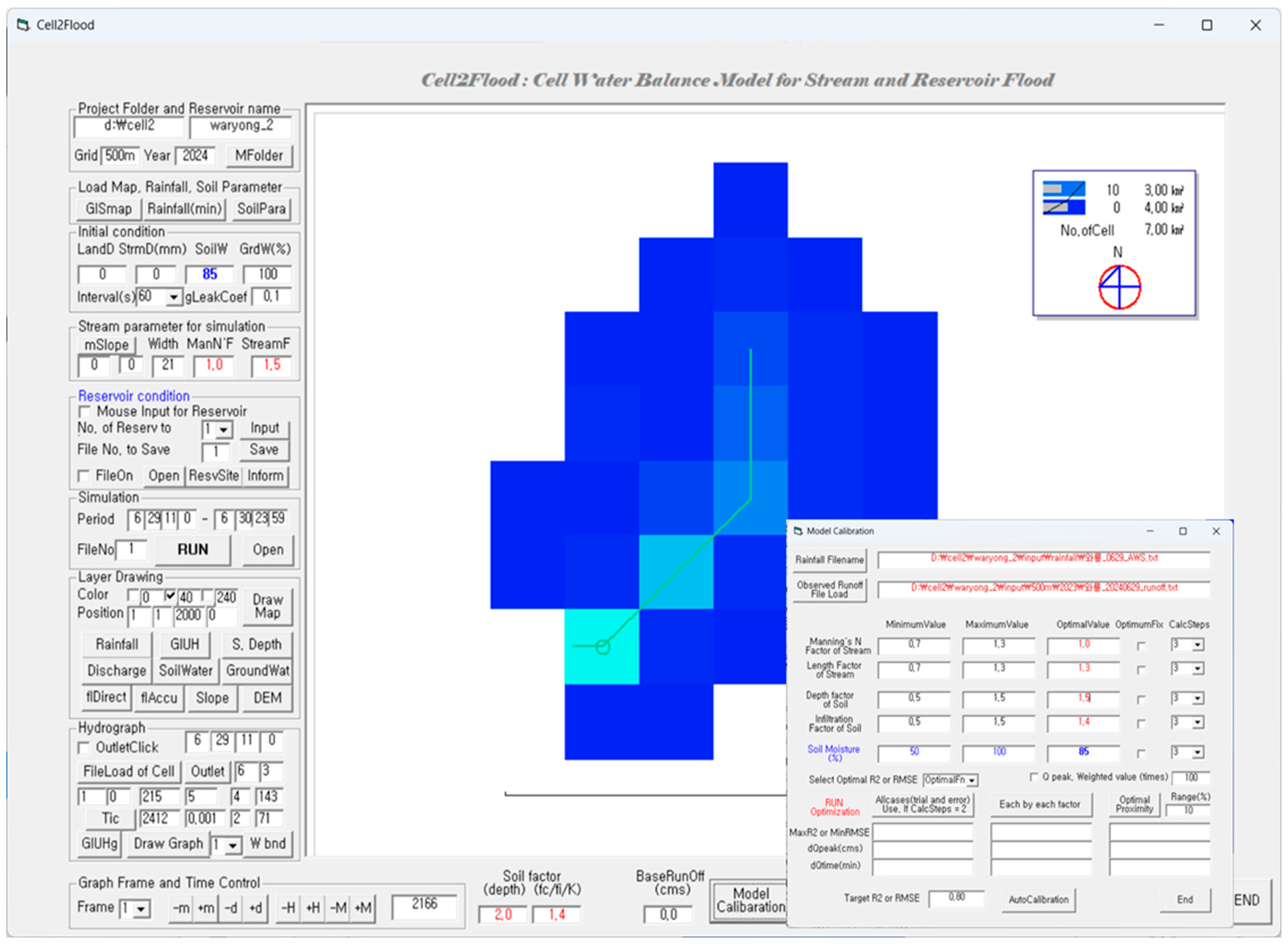
Cell2Flood simulates rainfall–runoff hydrologic flow on a three-layer conceptualization, surface flow, interflow, and groundwater, on a grid basis. Surface flow and interflow are modeled to occur in specific flow directions, whereas groundwater outflow can occur in all directions and is governed by a two-dimensional groundwater flow equation. The model functions independently of a Geographic Information System (GIS) engine, employing the ASCII format for all spatial input and output data. As shown in Figure 2, Cell2Flood provides a graphical user interface and incorporates an auto-calibration module developed using Visual Basic. Further developmental efforts are underway to create cloud-based web interfaces that enhance accessibility and functionality [20].
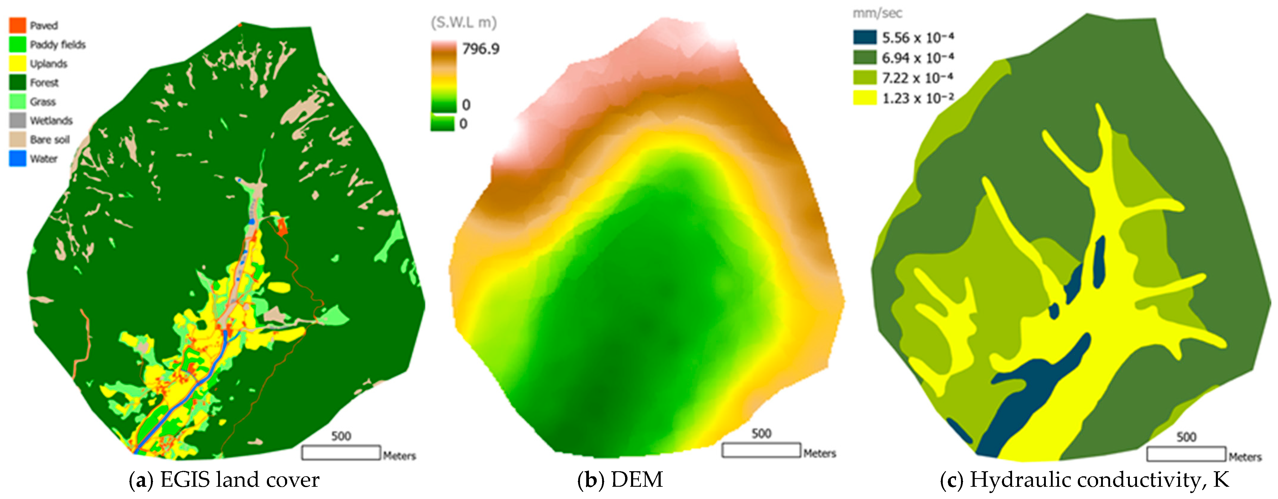
The model utilizes a suite of geospatial raster data, including a land cover map, detailed soil map, Digital Elevation Model (DEM), flow direction map, and flow accumulation map, including 10-min interval rainfall data stored in a text file. In this study, the land-cover map used was Level-2, which categorized land-cover features from the Environmental GIS (EGIS) of the South Korean Ministry of Environment [28]. Soil properties were derived from detailed soil maps (1:25,000 scale) of the National Institute of Agricultural Sciences (NAS) in South Korea, employing parameters such as effective soil depth, hydraulic conductivity, initial infiltration rate, and steady-state infiltration rate by soil texture to determine rainfall infiltration and soil moisture dynamics [29]. All data were resampled to a common 500 m spatial resolution and converted to an ASCII format (Figure 3). During data loading, the rainfall data in the text file were automatically parsed and transformed into an ASCII grid at 10-min intervals coinciding with the spatial extent of the other raster layers. The study area encompassed 30 valid data cells within an 8-row by 6-column grid, defined by the basin boundary and excluding any Null cells.

2.3. Preparation of Rainfall Inputs

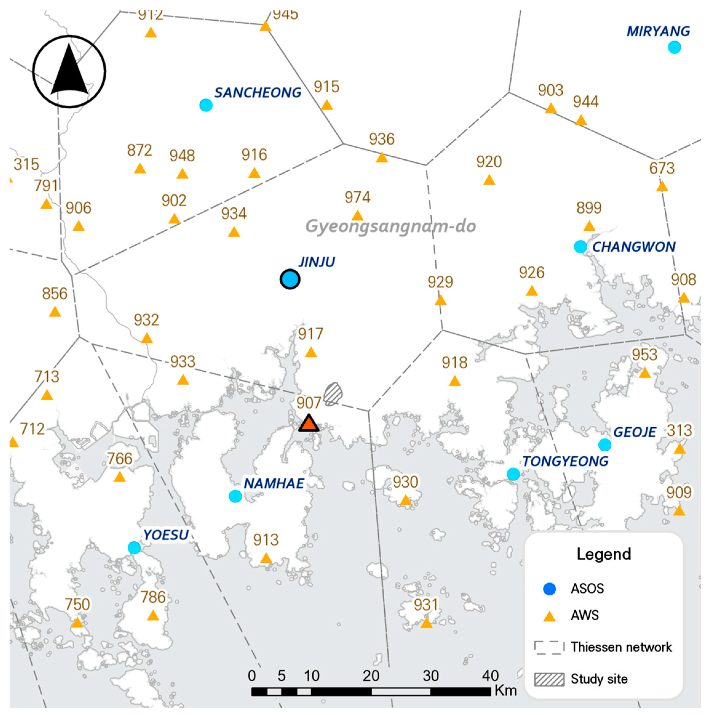
To assess the applicability of the rainfall input data to the Cell2Flood model in ungauged basins with limited hydrometric data, six distinct types of rainfall datasets, including on-site measurements, were generated for the model input. Initially, point-gauged rainfall data were collected from three sources, the sole on-site AWS within the target basin, the nearest AWS (Samcheonpo/907), and the governing ASOS station (Jinju/192), as determined using the Thiessen network method (Figure 4). Furthermore, three types of gridded rainfall data were generated: one interpolated from 39 ASOS stations surrounding the target area, another from 117 AWS stations, and the third based on Hybrid Surface Rainfall (HSR) radar data provided by the KMA. For spatial interpolation, inverse distance weighting (IDW), commonly adopted in hydrological studies [30], was applied at a spatial resolution of 500 m to align with the HSR data. Each dataset was maintained at a temporal resolution of 10 minutes. The HSR dataset was calibrated using KMA to account for the topographic complexity of the Korean Peninsula. The dataset was generated by synthesizing radar observations from 14 large dual-polarization radar stations, including a radar testbed dedicated to technological development, and was provided at temporal intervals as short as 5 min.
Rainfall events for testing were selected considering the availability of rainfall and runoff measurement data from the on-site AWS, as well as the presence of rainfall observations at ASOS (192) and AWS (907). The chosen events were 27 June 2023 (Event I), 9 August 2023 (Event II), and 29 June 2024 (Event III). Considering the variation in the start and end times of rainfall events across the observation stations, the time range for each event was standardized, as detailed in Table 1, to facilitate a consistent comparison of rainfall input data and ensure uniform temporal conditions for runoff simulation.

2.4. Evaluation Metrics for Correlation and Performance

To evaluate the differences and impacts of various rainfall products on the simulated runoff values, the following performance metrics were employed: Root Mean Square Error (RMSE), Nash–Sutcliffe Efficiency (NSE), Mean Absolute Error (MAE), Percent Bias (P-bias), Pearson correlation coefficient (Pearson’s r), and R-square [31].
The RMSE quantifies the difference between the observed values and their corresponding counterparts, with lower RMSE values signifying a closer correspondence between the datasets. A smaller value indicates a stronger alignment between the compared data.
R M S E = y y ^ 2 n
where y   i s   t h e   o b s e r v e d   v a l u e   a n d   y ^   i s   t h e   c o u n t e r p a r t   o r   s i m u l a t e d   v a l u e .
NSE is a widely used indicator for evaluating the goodness-of-fit between a pair of datasets. The NSE ranges from negative infinity to 1.0, with values closer to 1.0, indicating an optimal fit. Typically, an NSE value greater than 0.5 indicates satisfactory model performance [5].
  N S E = 1 i = 1 n y i y ^ i 2 i = 1 n y i y ¯ 2
where y ¯   is   t h e   a v e r a g e   o f   a l l   y   v a l u e s .
MAE is the average absolute difference between two datasets. Unlike other metrics, MAE does not involve squaring errors, thereby giving equal importance to all deviations. A smaller MAE indicates a closer alignment with the observation value.
M A E = 1 n y y ^
The P-bias measures the percentage difference between the observed data and other datasets, indicating the direction and magnitude of the bias in the comparison [32]. A positive P-bias value suggests that the estimation tends to undervalue the observed data, whereas a negative P-bias value indicates an overestimation.
P b i a s = i = 1 n y i y ^ i i = 1 n y i × 100 %
The coefficient of determination, R-square, describes the proportion of variance in one dataset that is explained by another dataset. An R-square value closer to one indicates a better fit, whereas a value closer to zero suggests that the dataset explains little of the variance in the reference dataset.
Pearson’s r is used to measure the linear relationship between two continuous variables. The value ranges from −1 to 1, with values closer to 1 or −1 indicating a stronger positive or negative correlation, respectively. A value of zero suggests no linear relationship between variables.
P e a r s o n s r = i = 1 n y i y ¯ y ^ i y ^ ¯ i = 1 n y i y ¯ 2 i = 1 n y i ^ y ^ ¯ 2
where y ^ ¯   is   t h e   a v e r a g e   o f   a l l   y ^ values.
Normalized Peak Error (NPE) and Peak Timing Error (PTE) indices were employed, focusing on short-term flood simulations. The NPE represents the relative difference between the simulated and observed peak flows and is expressed as a ratio to the observed peak. This underscores the accuracy of the model in replicating peak events, with lower values indicating a closer alignment between the predicted and observed peaks, thereby demonstrating better model performance in predicting peak flow.
N P E = max y ^ max y max y
where max( y ) is the observed peak flow and max( y ^ ) is the simulated peak flow.
PTE measures the difference between the observed and simulated peak times. A PTE value closer to zero indicates that the model accurately predicts the actual peak time [33].
P T E = t max y t max y ^
where t max y is the observed time-to-peak and t max y ^ is the simulated time-to-peak.

3. Results and Discussion

3.1. Comparison of Rainfall Inputs

3.1.1. Accumulated Rainfall

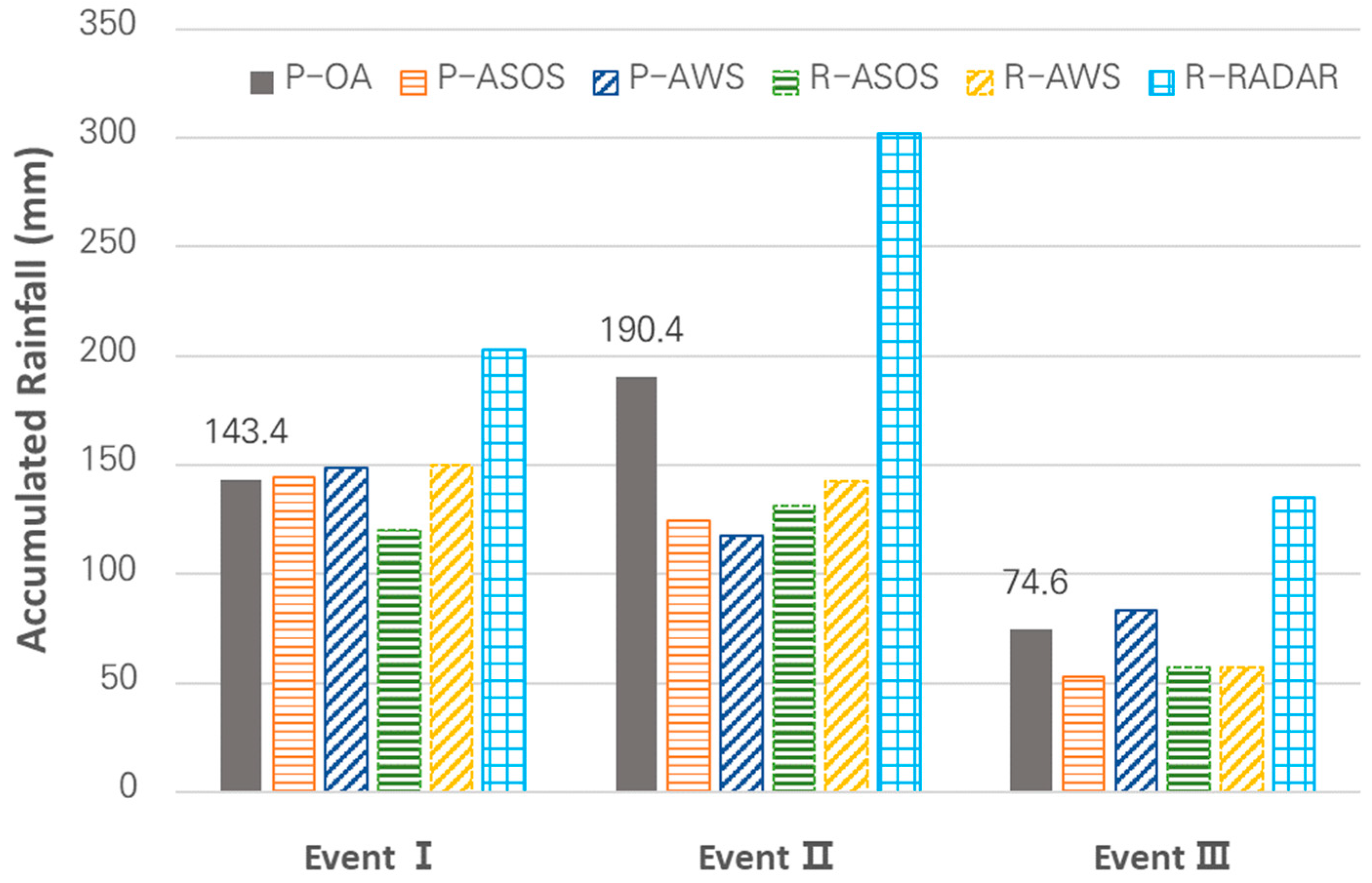
A comparative analysis of the accumulated rainfall across the six selected datasets was conducted to evaluate the uncertainty inherent in the rainfall inputs for hydrological modeling (Figure 5). At the basin observation point (P-OA), Event II, influenced by Typhoon Khanun, recorded the highest total rainfall at 190.4 mm, whereas Event III registered the lowest at 74.6 mm. Notably, across all three events, the point-gauged rainfall data (P-AWS) from the nearby Samcheonpo AWS and the basin-averaged rainfall (R-AWS) derived from the gridded dataset interpolating both the ASOS and AWS stations exhibited the closest alignment with the onsite AWS observations (P-OA). In Event II, wherein P-OA observed the highest rainfall, all datasets except the HSR radar-derived data (R-RADAR) underestimated the observed totals, with the most pronounced discrepancy occurring between P-OA and the other datasets. In contrast, R-RADAR consistently overestimated the accumulated rainfall across all events, particularly in Event III, where it reported 128.8 mm—approximately 1.7 times the value observed at P-OA (74.0 mm). Although the point-gauged P-AWS data and gridded R-AWS dataset appeared to be the most reliable inputs for modeling based on accumulated rainfall alone, the substantial variability observed between events underscored the need for a thorough examination of the spatiotemporal dynamics of rainfall across the study area.

3.1.2. Temporal Distribution of Rainfall

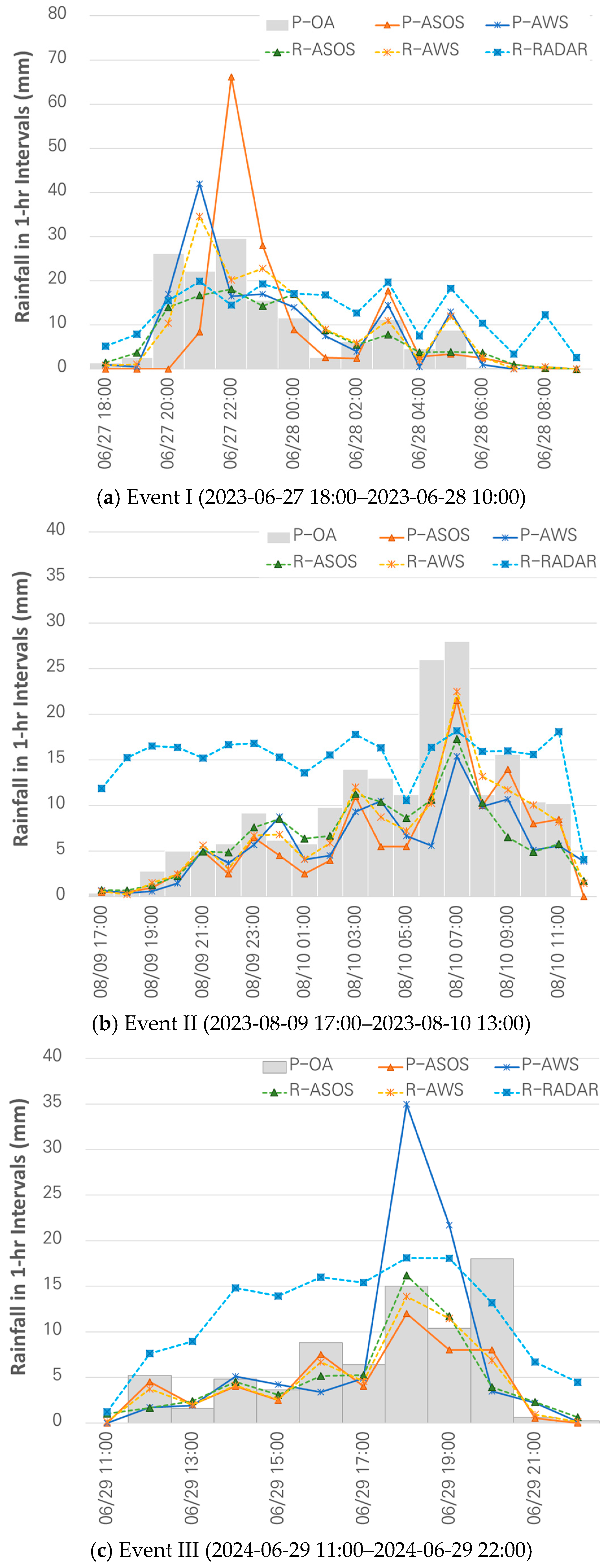
The hourly rainfall variation analysis for each event revealed different temporal distributions across rainfall inputs. In Event I, the point-gauged data from the P-AWS and the basin-averaged rainfall from the gridded R-ASOS dataset, which interpolated only the ASOS stations, showed the closest match with the on-site AWS observations (P-OA) (Figure 6a). P-OA and P-ASOS recorded peak rainfall simultaneously, whereas all other datasets recorded the peak 1 h earlier, between 22:00 and 23:00 on 27 June 2023. For Event II, as shown in Figure 6b, all rainfall datasets except the radar-based rainfall (R-RADAR), which exhibited minimal temporal variation, recorded a peak simultaneously between 07:00 and 08:00 on 10 August 2023, consistent with that of the P-OA. However, the maximum hourly rainfall across all rainfall inputs was lower than that of the P-OA. In Event III, all rainfall inputs, except P-OA, recorded a peak between 18:00 and 19:00 on 29 June 2024, 2 h earlier than P-OA (Figure 6c). Notably, despite its proximity to the study basin, P-AWS recorded a maximum hourly rainfall approximately 1.9 times higher than that of P-OA, suggesting substantial spatial inhomogeneity within the basin.
Across all events, the R-RADAR temporal discrepancies were less pronounced than those of the other datasets and exhibited relatively consistent patterns. Although this study utilized corrected and quality-controlled data from the KMA, the observed uncertainties appeared to be influenced by the topographic characteristics of the target basin and inherent errors in radar-based rainfall measurements. Although radar technology offers the advantage of real-time spatial coverage, it is less accurate than ground-based observations because it measures the relative rainfall intensity through radar reflectivity rather than directly measuring rainfall amounts. Radar-based rainfall measurement technology is inherently subject to several fundamental error factors, including calibration errors, variations in raindrop size, and anomalous propagation effects such as ground clutter and super-refraction, beam blockage, radar beam propagation angles, and beam ducting [1,9,16,34]. This suggests that although radar-derived data could be valuable for their spatial coverage, they require careful calibration and adjustment for local conditions to improve accuracy.

3.1.3. Rainfall Intensity

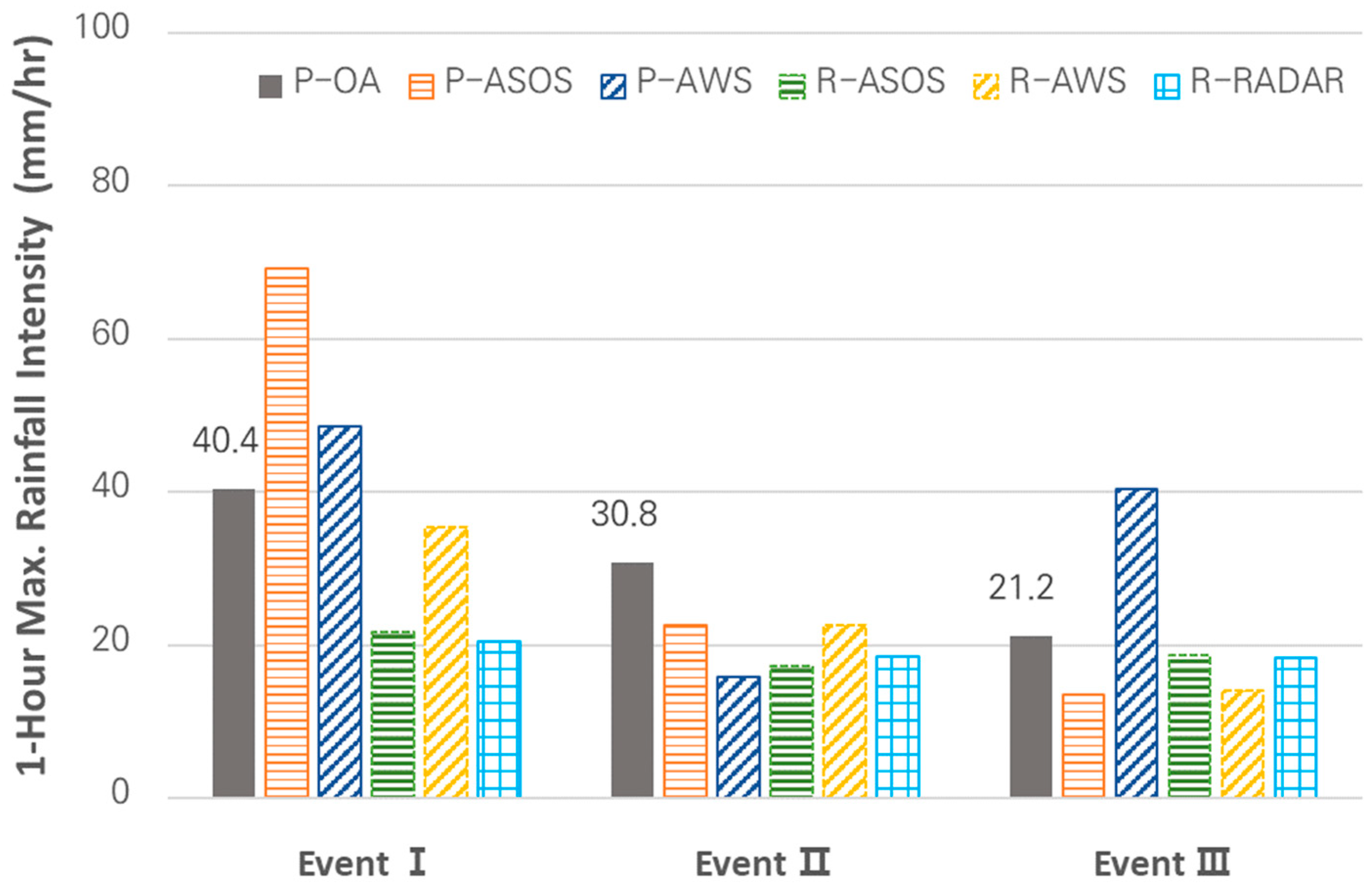
For the 1 h rainfall intensity, the maximum intensities at P-OA were 40.4 mm/h for Event I, 30.8 mm/h for Event II, and 21.2 mm/h for Event III (Figure 7). According to the KMA Special Weather Report, Event I was classified as an extreme rainfall event, with the Jinju ASOS recording more than 50 mm of rainfall within 1 h and more than 90 mm of accumulated rainfall over 3 h, which led to the issuance of a Heavy Rain Warning. In Event I, P-ASOS recorded the highest 1 h rainfall intensity among the rainfall inputs, whereas the gridded datasets, including R-RADAR, recorded lower maximum intensities than P-OA. A similar pattern was observed in Event II, where all rainfall inputs recorded lower accumulated rainfall and 1 h maximum rainfall intensity than in P-OA. Despite the influence of Typhoon Khanun, the lower intensities could be attributed to its weakening into a Tropical Storm (TS) as it passed over the southern region of the Korean Peninsula. For Event III, the 1 h maximum rainfall intensity was lower across all rainfall inputs compared to the other events, except for P-AWS. Notably, P-AWS, which recorded the lowest accumulated rainfall, exhibited a markedly higher maximum rainfall intensity than P-OA and the other rainfall inputs. The issuance of only a Strong Wind Advisory rather than a Heavy Rain Advisory or Warning in the KMA Special Weather Report for this region explained the lower accumulated rainfall and maximum rainfall intensity observed in Event III. Meanwhile, R-RADAR, which consistently recorded the highest accumulated rainfall across all events, exhibited relatively lower 1 h maximum rainfall intensities than the other inputs, with minimal variation between events. This suggests that the radar data captured fewer temporal fluctuations in rainfall intensity, likely due to their tendency to average intensity over larger areas and time intervals (Figure 6). This reveals their limitations in accurately capturing peak intensity events.

3.1.4. Spatial Distribution of Rainfall

In addition to the quantitative and temporal variability of rainfall, its spatial distribution significantly influences runoff. Consequently, the spatial variation in rainfall inputs at the time of the maximum 10-min rainfall at P-OA during each event was compared (Figure 8). The spatial distributions of R-ASOS, generated by IDW interpolation using only ASOS stations, and R-AWS, which incorporated AWS stations to enhance the density of observation points, were generally consistent across all events with respect to relative rainfall magnitude. However, an evident directional bias emerged, with higher rainfall interpolated to the north for Event I, southeast for Event II, and north for Event III. This directional bias was attributed to the uneven distribution of observation points and localized variations in rainfall. Despite the general consistency in spatial patterns, substantial quantitative differences were noted between R-ASOS and R-AWS, likely driven by variations in observation density and rainfall measurements among the gauges. Typically, when the density of rainfall observation points is low, it is challenging to adequately represent the overall rainfall over a basin, which leads to potential biases in the input data. Considering the small basin area, this study underscores the significant influence of the density of ground-based observation points on the accuracy of spatial interpolation.
In contrast, R-RADAR showed a distinctly different spatial distribution compared with R-ASOS and R-AWS. As previously noted, the quantitative and temporal discrepancies between the R-RADAR and ground measurements are shown in Figure 8. Radar-based rainfall estimates provide real-time coverage of large areas and are useful for runoff analyses that account for rainfall spatial heterogeneity. However, these estimates have been consistently criticized for overestimating or underestimating rainfall compared with ground observations, depending on the correction method and specific regional characteristics [5,9,35,36,37]. This demonstrates the necessity for careful calibration and integration with ground observations to improve the accuracy of radar-derived rainfall data.

3.1.5. Statistical Difference among Rainfall Inputs

The discrepancies between the observed rainfall at P-OA and the various rainfall input datasets are presented in Table 2. For Event I, the area-averaged rainfall from R-ASOS was determined to be most closely aligned with P-OA, whereas the point-gauged dataset P-ASOS showed lower errors and higher correlation compared with the other inputs in several error metrics (Pearson’s r = 0.68, RMSE = 2.05 mm). In Event II, the area-averaged rainfall from R-AWS demonstrated smaller differences compared with that from R-ASOS across multiple metrics, indicating that incorporating additional AWS stations improved the correlation. In addition, the R-AWS showed the closest match to the observed rainfall in all metrics (RMSE = 0.96 mm, Pearson’s r = 0.76, PTE = 0.0 min) without NPE, with a 31% lower estimation of peak rainfall. For Event III, P-ASOS exhibited the highest level of similarity to the observed data. Across all events, P-ASOS and R-ASOS consistently exhibited strong positive values for P-bias, indicating that they were underestimated compared with P-OA.
In contrast, the area-averaged rainfall from R-RADAR showed the greatest deviations from the P-OA across all events. The R-squared values were consistently below 0.2, indicating weak correlations, whereas the P-bias values exceeded −41.6%, indicating a substantial overestimation of rainfall compared to the observed data. Figure 5, Figure 6, Figure 7 and Figure 8 show that R-RADAR consistently showed significant deviations from the on-site observations across all events, confirming its limited reliability without further calibration. According to the studies by Lyu et al. [38] and Lee et al. [8], the HSR data used in this study, although corrected with the latest technology, exhibited correlation coefficients with observed values ranging from 0.52 to 0.78 and mean relative errors (MREs) exceeding 30 mm/h. Although the HSR simulated ground rainfall was within a 15% margin of error, its accuracy varied significantly depending on rainfall intensity and pattern.
Table 2 lists the discrepancies among the different rainfall inputs. Point-gauged datasets (P-ASOS and P-AWS) and spatially interpolated datasets (R-ASOS and R-AWS) can generally be considered to provide more consistent and reliable estimates than radar-derived data (R-RADAR). However, the differences observed across various events suggest that the accuracy of these datasets could be highly dependent on the specific conditions of each rainfall event, such as the intensity, duration, and spatial distribution.

3.2. Runoff Simulation with On-Site Calibrated Parameters

3.2.1. On-Site Parameter Calibration of Cell2Flood

A physically based rainfall–runoff model such as Cell2Flood requires parameter optimization that accurately reflects the characteristics of a specific basin. However, because of the inherent uncertainties within such hydrological models, parameter calibration using historical observations can vary depending on the flow dynamics of an event [13]. In this study, as shown in Table 3, the parameters were first calibrated based on P-OA to satisfy both Events I and II and then verified with Event III to ensure that the model adequately replicated the observed conditions; the results of each performance were discussed in the following Section 3.2.2, Section 3.2.3 and Section 3.2.4. A high nratio (25.0) indicated a significant adjustment to streamflow, which was necessary because of the rapid response of the basin to intense rainfall events. Similarly, the relatively low Dratio (0.4) suggested a limited effective soil depth, which could affect the infiltration rates and the timing of peak flow. During the calibration process, NPE and PTE were considered, including peak discharge and time-to-peak, critical hydrological indicators for short-term flood events, which were the primary focus of this study.
The event-dependent initial conditions, including the initial soil moisture (%) and initial groundwater level relative to surface elevation (%), were calibrated individually for each event using a trial-and-error method, as summarized in Table 4. These calibrated conditions were then uniformly applied to all simulations with varying rainfall inputs to ensure consistent baseline conditions across scenarios.

3.2.2. Temporal Variations in Runoff by Rainfall Inputs

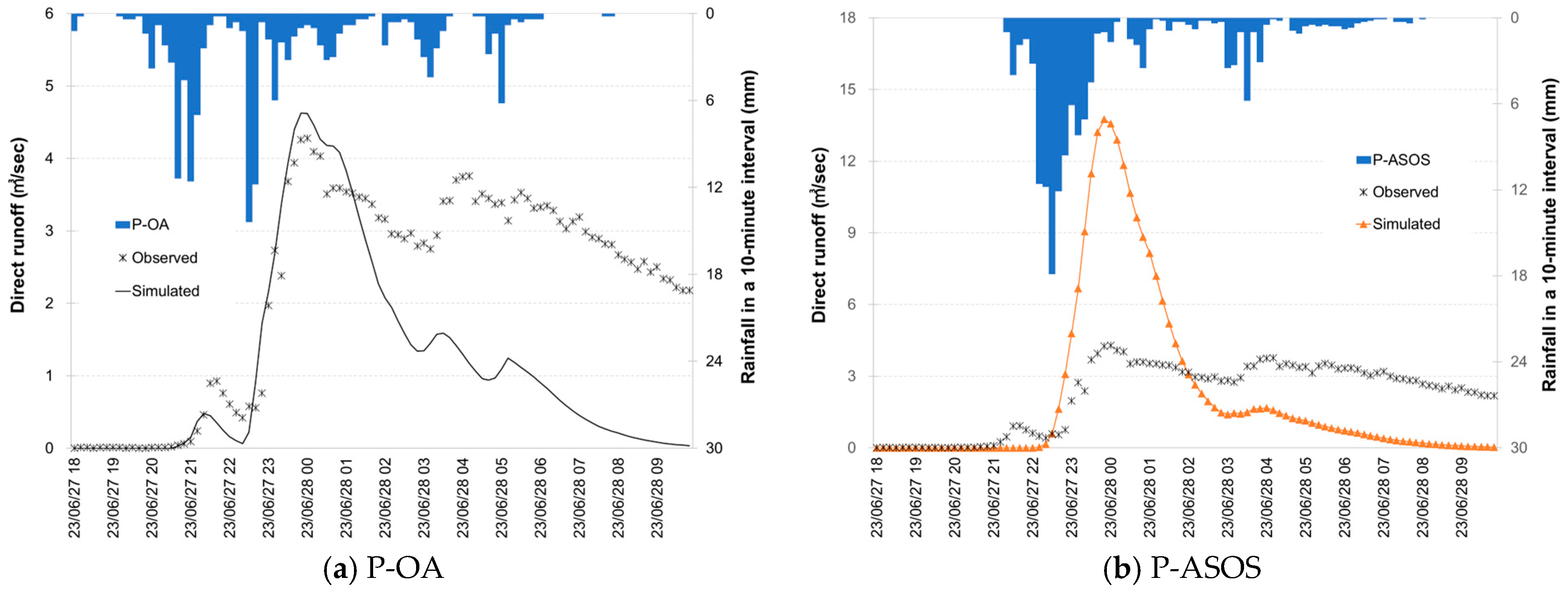
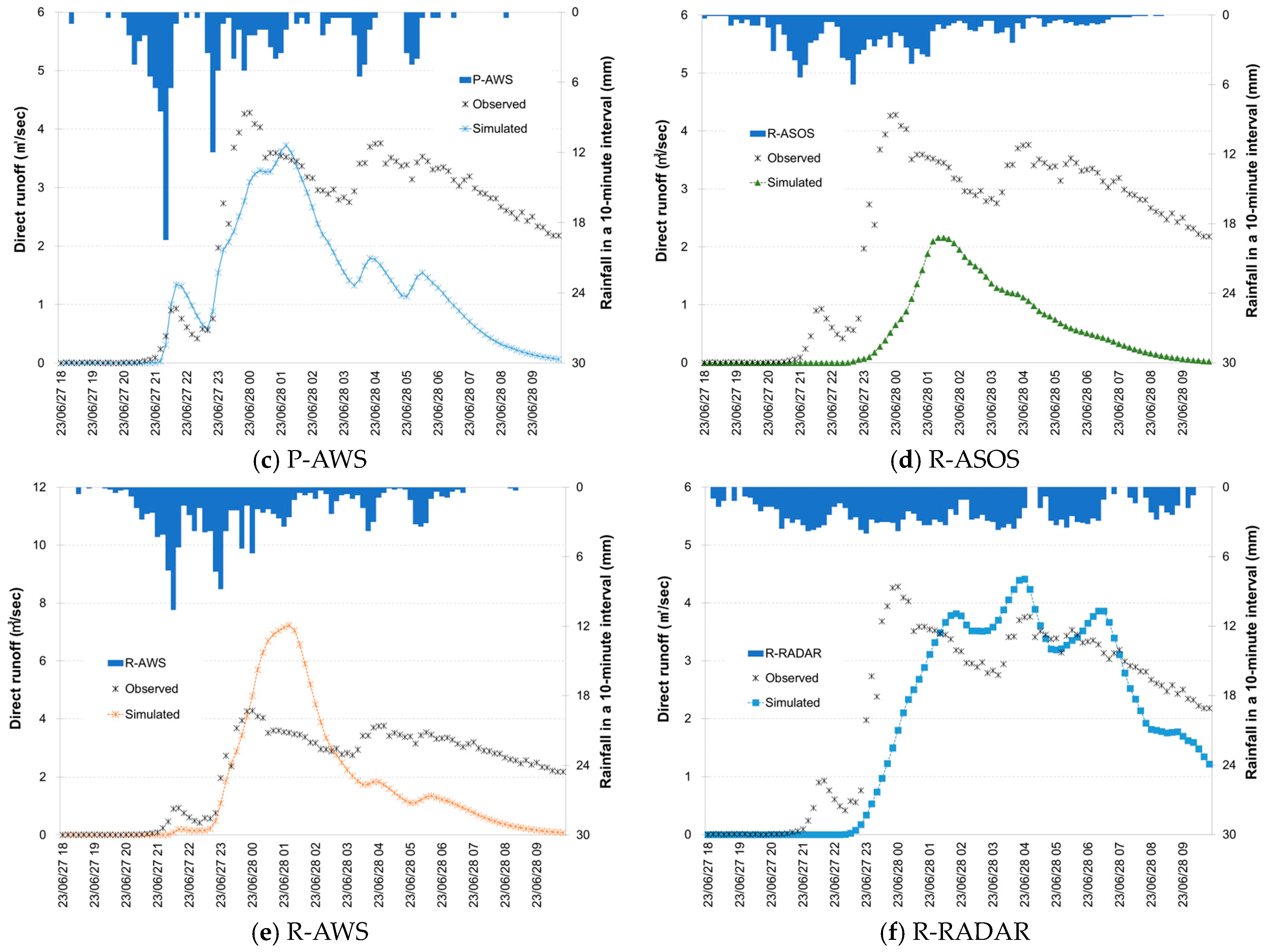
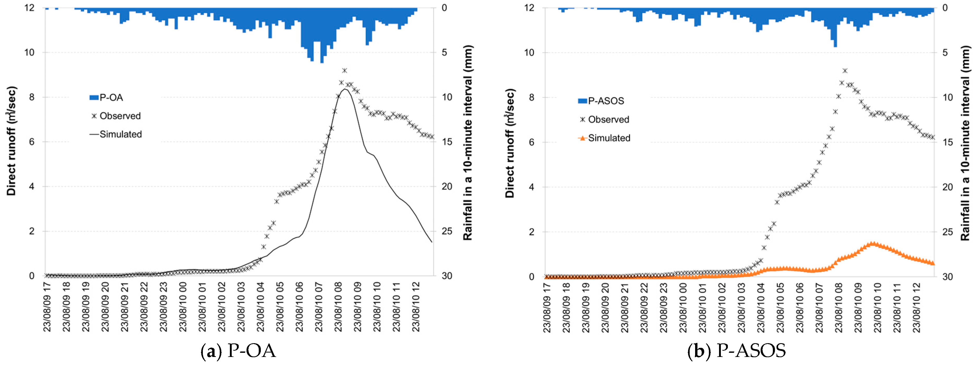
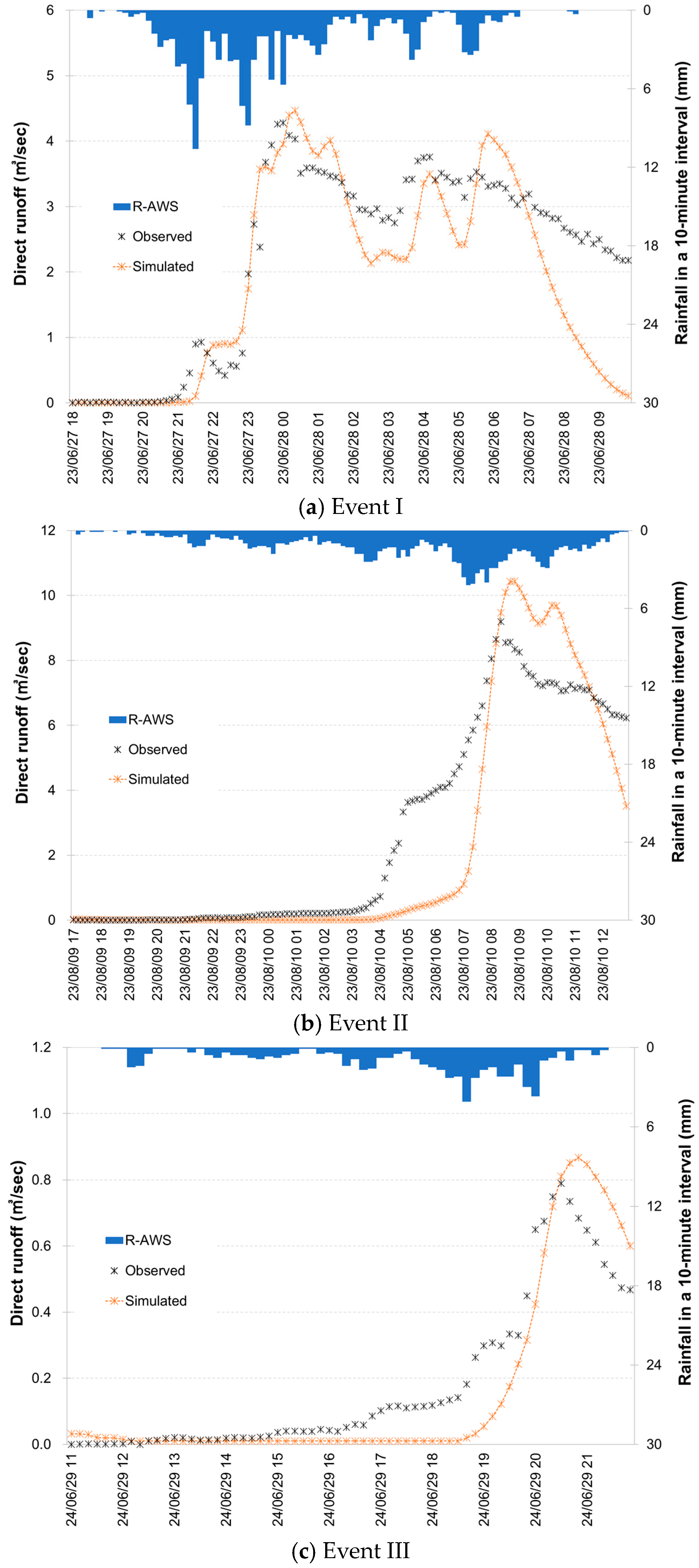
By applying the parameters from Table 3 and Table 4, the runoff variations for each event were simulated using Cell2Flood under identical conditions across all rainfall inputs (Figure 6, Figure 7 and Figure 8). Variations in rainfall intensity, timing, and spatial distribution among the inputs caused significant deviations in the simulated runoff compared with the observed measurements. In Figure 9, for Event I, except for R-RADAR, the temporal patterns of the rainfall inputs largely resembled those of P-OA. However, the interpolated datasets R-ASOS and R-AWS showed reduced temporal fluctuations in rainfall intensity. Although the rainfall amounts and intensities for R-AWS were higher than those for R-ASOS, as shown in Figure 5, Figure 6 and Figure 7, the runoff simulated with R-AWS tended to be overestimated relative to the observed values, whereas the runoff simulated with R-ASOS was consistently underestimated.
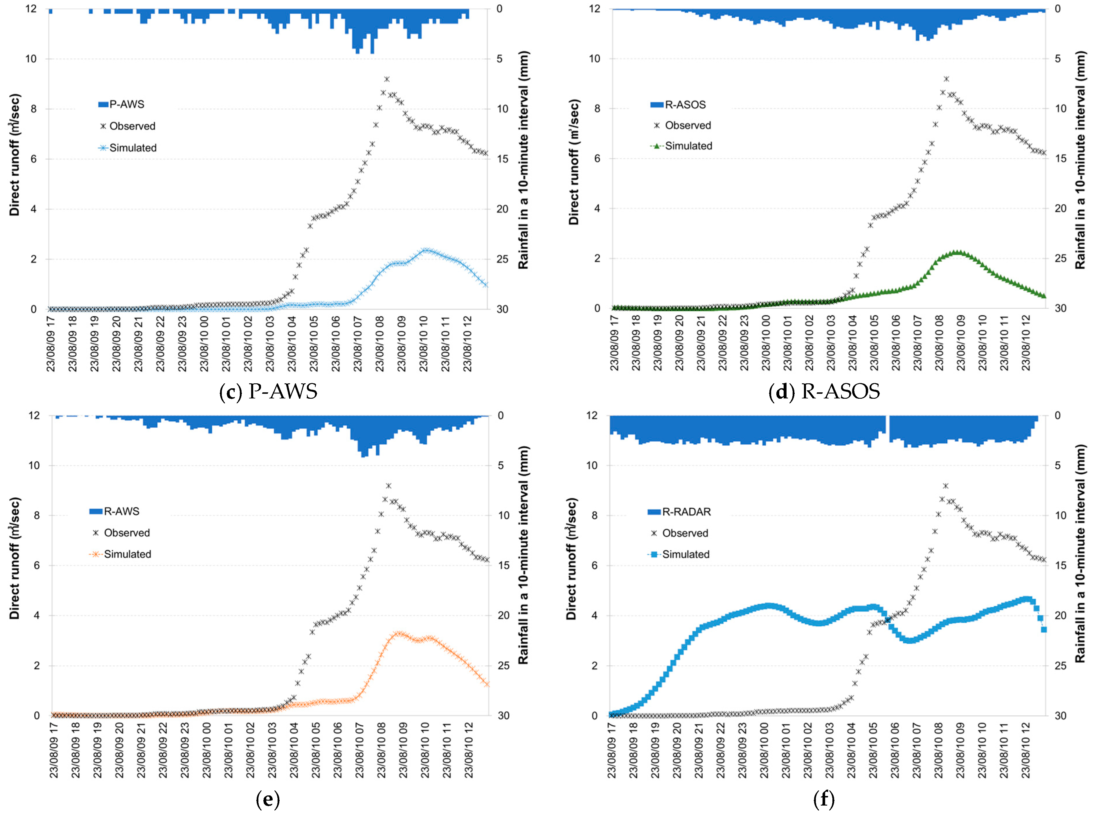
In Event II (Figure 10), all rainfall datasets, except R-RADAR, showed temporal patterns that corresponded well with the observed data but produced significantly lower simulated runoff than the actual measurements. This underestimation was likely due to the lower cumulative rainfall and reduced peak intensity compared with those of P-OA. Similar reasoning explained the underpredicted runoff observed in Figure 9d in the R-ASOS dataset, which showed diminished rainfall characteristics. For R-RADAR during Event II, the rainfall variation exhibited an anomalously steady intensity from the onset, unlike other datasets, including P-OA, which featured an initial period of low rainfall followed by a later increase (Figure 10f). The runoff simulated with R-RADAR increased earlier than the observed runoff and deviated substantially, reflecting a distinct temporal response pattern that did not align with on-site measurements.
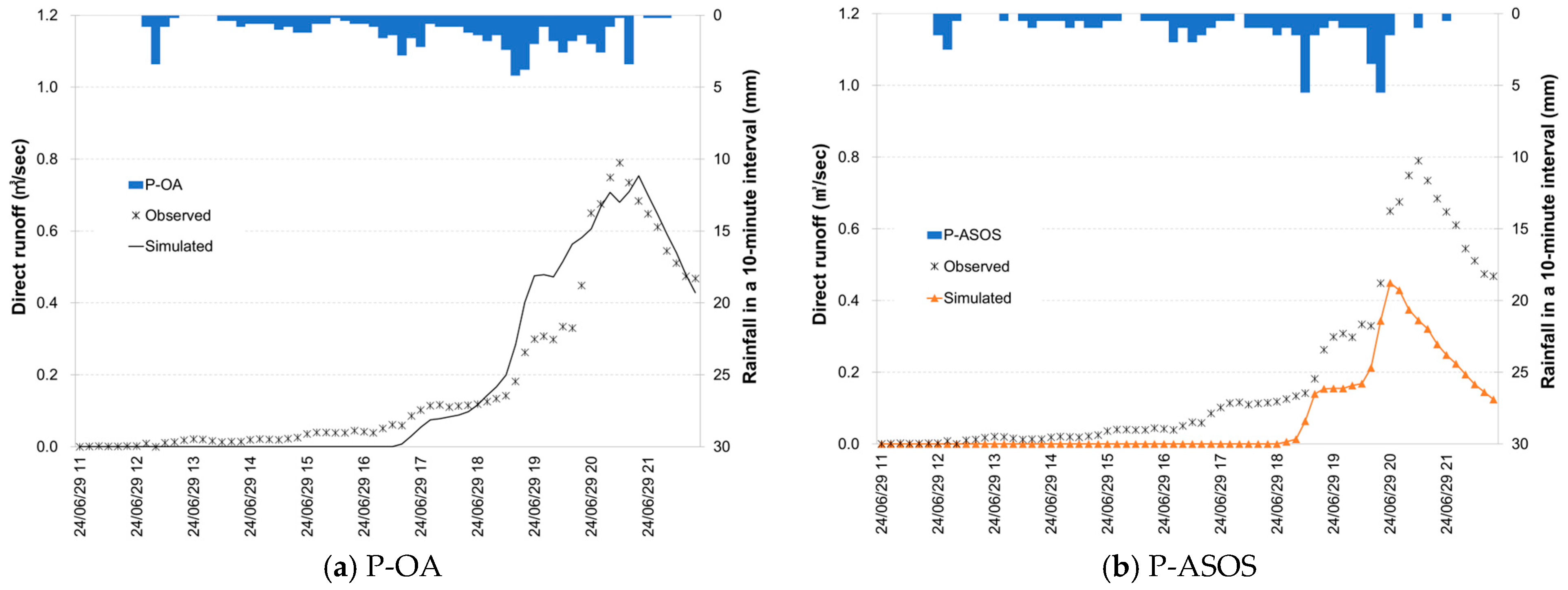
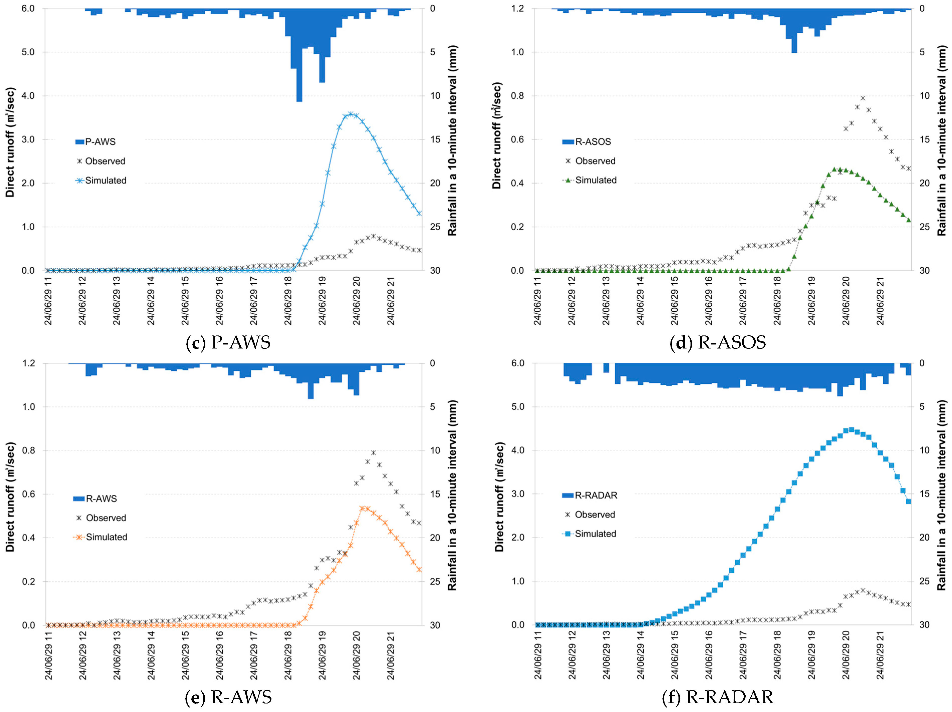
For Event III, which recorded the lowest rainfall and runoff among all events, the datasets with higher accumulated rainfall than P-OA, such as P-AWS and R-RADAR, overpredicted the runoff (Figure 11). Conversely, despite capturing a temporal pattern closely aligned with the observed data, P-ASOS, R-ASOS, and R-AWS consistently underpredicted the runoff because of their lower accumulated rainfall and intensity relative to P-OA. R-RADAR consistently showed significant temporal deviations and patterns of over- or underestimation across different events, mirroring the limitations discussed in previous sections.

3.2.3. Peak Flow by Rainfall Inputs

The runoff simulation results showed considerable variations in peak discharge and timing, which were closely linked to differences in rainfall inputs, as summarized in Table 5. The P-AWS exhibited considerable discrepancies in the simulated peak discharges across all events, with significant variations in the time-to-peak ranging from 40 to 112 min. These errors, reflected by a relatively high RMSE value of 3.33 mm and a low R-square under 0.25, as presented in Table 2, suggest that the P-AWS struggled to accurately capture the spatial variability of rainfall despite its proximity to the study basin. Similarly, the R-RADAR simulation resulted in substantial inaccuracies, including a 310 min delay in time-to-peak in Event I and a 5.7-fold overestimation of peak discharge in Event III. These insignificant deviations were consistent with the low R-square of 0.17 and poor NSE scores ranging from −0.31 to 0.06. Regardless of the accumulated rainfall amount, the simulated peak discharge across all events remained within a range of approximately 4–5 m3/s. As shown in Figure 9f, Figure 10f and Figure 11f, the temporal variation in R-RADAR was less dynamic compared with other rainfall inputs, which is also evident in Figure 7, likely because of its limitations in capturing rapid changes in rainfall intensity and timing.
Overall, the differences in the runoff simulations were primarily attributed to variations in the rainfall inputs. Excluding P-OA, the rainfall datasets that produced runoff simulations closest to the observed values differed between events. No single rainfall input consistently demonstrated meaningful similarities in both peak discharge and time-to-peak across all events, indicating that the reliability of each rainfall input was event-dependent and highly variable. These findings reveal the need to select and calibrate suitable rainfall inputs to improve the accuracy of hydrologic models such as Cell2Flood, which is crucial for effective flood forecasting and management.

3.2.4. Evaluation of the Runoff Simulations

Several performance metrics were considered for evaluating the differences and effects of various rainfall products on the simulated runoff values (Table 6). In Event I, R-RADAR performed relatively well across most metrics, except for PTE, which showed a substantial deviation of −300 min, making its temporal accuracy questionable. Nonetheless, the R-RADAR simulation exhibited a slight deviation in the peak discharge, with an NPE of 0.03, even outperforming the P-OA. However, in Events II and III, the performance of R-RADAR deteriorated significantly, with high RMSE values of 3.06 and 2.13 m3/s, respectively, and large P-bias of −98.78% and −825.36%.
In contrast, the R-AWS demonstrated the highest correlation with the observed values in Event II, showing superior performance in terms of RMSE, NSE, P-bias, and MAE. The R-square value was also relatively high at 0.86, and although NPE and PTE were not the lowest, they still showed relatively minor discrepancies. R-AWS maintained a comparable level of performance in Event III, with the lowest RMSE of 0.11 m3/s, an NSE of 0.80, and the highest R-square of 0.96 among all rainfall datasets, excluding P-OA. Additionally, the MAE was only 0.08 m3/s, and both NPE and PTE were −0.32 and 20.0 min, respectively, closely aligned with the observed runoff patterns, indicating that R-AWS effectively captured the temporal and spatial variability in runoff. The evaluation results showed that the no-rainfall input consistently provided the most accurate simulation across all events. The performance of each dataset varied depending on the specific characteristics of each rainfall event, such as intensity, duration, and spatial distribution.

3.3. Runoff Simulation with Input-Specific Calibrated Parameters

3.3.1. Parameter Calibration for Each Rainfall Input

Rainfall inputs vary in spatial and temporal resolution and accuracy; therefore, using the same parameters for different rainfall datasets can reduce the accuracy of the simulated outcomes owing to the unique characteristics of each dataset. The model can better account for each dataset’s distinct features and uncertainties by calibrating the parameters specific to each input. Some rainfall inputs performed better for specific events than others, indicating that the model’s response varied depending on the data characteristics. In this study, input-specific parameter calibration was performed to optimize model performance and improve the accuracy of short-term runoff modeling for each rainfall dataset. The calibration primarily focused on the peak discharge and time-to-peak critical performance indicators for flood events, whereas other metrics, such as NSE, RMSE, P-bias, and MAE, were used as supplementary indicators to validate the overall model performance. The input-specific calibrated parameters for each rainfall dataset obtained through numerous trials and adjustments are summarized in Table 7. The parameter settings varied considerably among the different rainfall inputs, with particularly noticeable differences in nratio and Aratio compared with the onsite calibrated parameters in Table 3. Both nratio and Aratio values were reduced to minimize peak discharge and time-to-peak errors (Table 6). A lower nratio, which serves as a proportional constant for Manning’s roughness coefficient in the Cell2Flood model, resulted in increased flow rates and velocities. Similarly, a smaller Aratio, which determines the criteria for dividing river reaches, resulted in longer river sections with reduced travel times, thereby advancing the timing of the peak flow.

3.3.2. Evaluation of Runoff Simulations with Input-Specific Calibrated Parameters

The results of the simulations with input-specific calibrated parameters for each rainfall dataset are shown in Figure 12, Figure 13, Figure 14, Figure 15 and Figure 16.
As shown in Table 8, most performance metrics improved compared with the results obtained using the on-site calibrated parameters listed in Table 6. Although R-AWS showed the best overall performance with the on-site calibration shown in Table 6, the application of different calibration parameters to each rainfall dataset resulted in P-ASOS having the lowest error. For the event averages, P-ASOS demonstrated an RMSE of 0.57 m3/s, an R-square of 0.90, an NPE of 0.03, and a PTE of −22.3 min, reflecting the best or nearly the best performance across all indicators. In contrast, P-AWS produced the poorest runoff simulation, with an average event RMSE of 1.18 m3/s, an R-square of 0.54, a P-bias of 31.34%, and an NPE of 0.12. Although R-RADAR showed improvements across all metrics, it still exhibited significant errors in certain events, such as a P-bias which was as high as −29.03% and a PTE of −219 min, indicating limitations in the rainfall data that cannot be fully resolved through parameter calibration alone. Consequently, for the Waryong Reservoir Basin, the point-gauged rainfall input from the ASOS (P-ASOS) was more effective for short-term runoff modeling than the R-AWS data, which relied on IDW spatial interpolation using the maximum available surrounding meteorological data.

4. Summary and Conclusions

Accurate rainfall data are essential for predicting reservoir inflows, scheduling water releases, and maintaining sufficient storage capacity to mitigate flood risks while ensuring a stable water supply for irrigation. Inaccurate rainfall data can lead to premature or delayed water release, compromising dam safety and increasing downstream flood risk. Considering these challenges, this study evaluated the impacts of different rainfall input types on short-term runoff simulations using the Cell2Flood model for the Waryong Reservoir Basin in South Korea. By analyzing six types of rainfall data—on-site gauge measurements, spatially interpolated data from the ASOS and AWS stations (R-ASOS and R-AWS), and HSR data from the Korea Meteorological Administration—across three distinct rainfall events, this study aimed to identify the datasets that provide the most reliable inputs for effectively managing agricultural reservoirs, such as the study site.
Among the rainfall datasets, the P-ASOS station, which provided the most extensive record of rainfall observations for the study basin, exhibited cumulative rainfall and 1 h maximum rainfall intensity values most similar to those of the on-site observations (P-OA) and second only to the geographically closest P-AWS data. However, when examining the 10-min interval rainfall data, P-ASOS exhibited better alignment with P-OA than P-AWS for most metrics. Although P-AWS was expected to provide the most accurate representation of on-site rainfall owing to its proximity, it had lower Pearson’s r values and higher errors in the RMSE and other metrics, resulting in the largest discrepancies in runoff simulations, except when compared with R-RADAR. This finding highlights that spatial variability in rainfall can be significant even within small regions. Moreover, when using the onsite (P-OA) calibrated parameters, runoff simulations with P-ASOS data resulted in relatively smaller errors than those with P-AWS data. However, substantial inter-event variations and time-to-peak delays of up to 89 min led to error margins beyond acceptable levels. In contrast, adjusting the calibration to fit the characteristics of the P-ASOS data allowed for more accurate runoff simulations compared to other rainfall inputs, including P-AWS, with the smallest inter-event variations and peak discharge errors maintained within a 4% margin.
In the runoff simulations of the Cell2Flood model using spatially interpolated raster inputs, such as R-AWS and R-ASOS, the application of on-site calibrated parameters showed that R-AWS provided slightly more accurate results than R-ASOS. Even when rainfall input-specific optimized parameters were applied, slight differences were observed depending on the event and metrics; however, the event-averaged performance indicated that R-AWS outperformed R-ASOS. Meanwhile, the R-RADAR data, which were originally produced and provided in raster format, showed the most significant deviations from the observed values, often overestimating rainfall amounts and resulting in higher errors in runoff simulations under on-site-calibrated parameters. Although applying parameters specifically calibrated to R-RADAR inputs improved the results across all metrics, the overwhelming errors in the time-to-peak remained insurmountable. The radar-synthesized rainfall data exhibited significant uncertainties in matching the actual rainfall distributions, making it challenging to reduce errors despite hydrological parameter calibration (Figure 16).
Considering the short-term runoff characteristics of peak discharge and time-to-peak, this study found that P-ASOS, with peak discharge errors of less than 0.04 m3/s across all events, and R-AWS, with an average time-to-peak error within 20 min, could be prioritized as preferred rainfall inputs for the Cell2Flood model. However, when focusing solely on Events 1 and 2, which were characterized by intense rainfall and typhoon threats, the P-AWS and R-AWS were recommended as the primary inputs for flood management models because of their smaller errors in peak discharge and time-to-peak, along with lower inter-event variability.
Overall, this study demonstrated that although calibrating model parameters to different rainfall inputs could help to simulate the observed runoff in the Waryong Reservoir Basin, the inherent limitations of each rainfall dataset substantially influenced the accuracy of the runoff modeling. These findings emphasize the need to carefully consider the specific physical and meteorological characteristics of a basin when selecting rainfall data to enhance the reliability of hydrological models. The results suggest that regardless of the rainfall–runoff model mechanics or parameter calibration techniques used, choosing the most appropriate rainfall input for a given basin remains crucial for achieving accurate flood predictions. Furthermore, a comprehensive evaluation of diverse rainfall datasets is essential to understand the scale and nature of the uncertainties inherent in hydrological modeling and to improve the interpretation and application of model outputs for effective flood management.
However, the scope of this study was constrained by the limited number of rainfall events analyzed, particularly the absence of extreme, high-intensity storms critical for assessing reservoir management under diverse conditions. Future research should broaden the range of rainfall events, particularly those involving severe weather conditions, and utilize multiple modeling approaches to enhance the robustness and applicability of the findings. Additionally, refining radar datasets, such as HSR, to better capture local rainfall patterns and explore advanced data integration techniques could further improve runoff predictions, ultimately aiding in more effective management of agricultural reservoirs.

Author Contributions

Conceptualization, M.-W.J.; methodology, M.-W.J.; model correction and validation, D.-S.K.; validation, M.-W.J. and W.-H.N.; formal analysis, H.K.; investigation, H.K.; writing—original draft preparation, H.K.; writing—review and editing, M.-W.J.; visualization, H.K.; supervision, M.-W.J.; project administration, M.-W.J.; funding acquisition, D.-S.K., W.-H.N. and M.-W.J. All authors have read and agreed to the published version of the manuscript.

Funding

This research was funded by the Korea Institute of Planning and Evaluation for Technology in Food, Agriculture, and Forestry (IPET), grant number RS-2022-IP322078.

Data Availability Statement

Data collected for the study can be made available upon request.

Conflicts of Interest

The authors declare no conflicts of interest.

References

  1. Hu, C.; Liu, C.; Yao, Y.; Wu, Q.; Ma, B.; Jian, S. Evaluation of the impact of rainfall inputs on urban rainfall models: A systematic review. Water 2020, 12, 2484. [Google Scholar] [CrossRef]
  2. Hyun, J.H.; Park, H.; Chung, G. Effects of the difference between ASOS and AWS data on runoff characteristics. J. Korean Soc. Hazard Mitig. 2019, 19, 443–449. [Google Scholar] [CrossRef]
  3. Byaruhanga, N.; Kibirige, D.; Gokool, S.; Mkhonta, G. Evolution of flood prediction and forecasting models for flood early warning systems: A scoping review. Water 2024, 16, 1763. [Google Scholar] [CrossRef]
  4. Vaes, G.; Willems, R.; Berlamont, J. Rainfall input requirements for hydrological calculations. Urban Water 2001, 3, 107–112. [Google Scholar] [CrossRef]
  5. Palanisamy, B.A. Evaluation of SWAT Model—Subdaily Runoff Prediction in Texas Watersheds. Master’s Thesis, Texas A&M University, College Station, TX, USA, May 2006. [Google Scholar]
  6. Tramblay, Y.; Bouvier, C.; Ayral, P.A.; Marchandise, A. Impact of rainfall spatial distribution on rainfall-runoff modelling efficiency and initial soil moisture conditions estimation. Nat. Hazards Earth Syst. Sci. 2011, 11, 157–170. [Google Scholar] [CrossRef]
  7. Shakti, P.C.; Nakatani, T.; Misumi, R. The role of the spatial distribution of radar rainfall on hydrological modeling for an urbanized river basin in Japan. Water 2019, 11, 1703. [Google Scholar] [CrossRef]
  8. Lee, M.; Lee, C.; Yoo, Y.; Kwak, J.; Kim, H.S. Evaluation of hydrological applicability for rainfall estimation algorithms of dual-polarization radar. J. Korea Water Resour. Assoc. 2021, 54, 27–38. [Google Scholar]
  9. Ahn, S.R.; Jang, C.H.; Kim, S.H.; Han, M.S.; Kim, J.H.; Kim, S.J. Discussion for the effectiveness of radar data through distributed storm runoff modeling. J. Korean Soc. Agric. Eng. 2013, 55, 19–30. [Google Scholar]
  10. Ahn, S.R.; Jung, C.G.; Kim, S.J. A study on the effectiveness of radar rainfall by comparing with flood inundation record map using KIMSTORM (Grid-based KIneMatic Wave STOrm Runoff Model). J. Korea Water Resour. Assoc. 2015, 48, 925–936. [Google Scholar] [CrossRef]
  11. Vieux, B.E.; Park, J.H.; Kang, B. Distributed hydrologic prediction: Sensitivity to accuracy of initial soil moisture conditions and radar rainfall input. J. Hydrol. Eng. 2009, 14, 671–689. [Google Scholar] [CrossRef]
  12. Jang, D.W.; Kim, D.K.; Kim, Y.S.; Choi, W.I. Application of SWAT model considering spatial distribution of rainfall. J. Wetl. Res. 2018, 20, 94–103. [Google Scholar]
  13. Kim, J.H.; Song, Y.H.; Chung, E.S. Uncertainty of future runoff projection according to SSP scenarios and hydrologic model parameters. J. Korea Water Resour. Assoc. 2023, 56, 35–43. [Google Scholar]
  14. Piadeh, F.; Behzadian, K.; Alani, A.M. A critical review of real-time modelling of flood forecasting in urban drainage systems. J. Hydrol. 2022, 607, 127476. [Google Scholar] [CrossRef]
  15. Shin, H.J.; Lee, C.; Kim, G.; Kong, J.Y. Sensitivity analysis of precipitation and reservoir storage under climate change for agricultural reservoirs in South Korea. Water 2019, 11, 2578. [Google Scholar]
  16. Ahmed, S.I.; Rudra, R.; Goel, P.; Khan, A.; Gharabaghi, B.; Sharma, R. A comparative evaluation of using rain gauge and NEXRAD radar-estimated rainfall data for simulating streamflow. Hydrology 2022, 9, 133. [Google Scholar] [CrossRef]
  17. Thorndahl, S.; Einfalt, T.; Willems, P.; Nielsen, J.E.; ten Veldhuis, M.C.; Arnbjerg-Nielsen, K.; Rasmussen, M.R.; Molnar, P. Weather radar rainfall data in urban hydrology. Hydrol. Earth Syst. Sci. 2017, 21, 1359–1380. [Google Scholar] [CrossRef]
  18. Thorndahl, S.; Nielsen, J.E.; Rasmussen, M.R. Estimation of storm-centred areal reduction factors from radar rainfall for design in urban hydrology. Water 2019, 11, 1120. [Google Scholar] [CrossRef]
  19. Kim, D.; An, H.; Jang, M.; Kim, S. Development for a distributed hydrological model considering hydrological change. Korean J. Agri. Sci. 2017, 45, 521–532. [Google Scholar] [CrossRef]
  20. Kim, D. Development of Spatiotemporal Real-Time Runoff and Flood Prediction System for Agricultural Reservoirs; Korea Institute of Planning and Evaluation for Technology in Food, Agriculture, and Forestry: Jeollanam-do, Republic of Korea, 2022; pp. 47–61. [Google Scholar]
  21. Rural Agricultural Water Resource Information System (RAWRIS). Available online: https://rawris.ekr.or.kr (accessed on 25 September 2024).
  22. Korean Soil Information System (KSIS). Available online: https://soil.rda.go.kr (accessed on 25 September 2024).
  23. Chung, H.W.; Kim, S.J.; Choi, J.Y.; Kim, D.S. GIS application model for temporal and spatial simulation of surface runoff from a small watershed. J. GIS Assoc. Korea 1995, 3, 135–146. [Google Scholar]
  24. Beven, K. Rainfall-Runoff Modelling: The Primer, 2nd ed.; Wiley-Blackwell: Oxford, UK, 2012; pp. 40–44. [Google Scholar]
  25. Dwarakish, G.S.; Ganasri, B.P.; De Stefano, L. Impact of land use change on hydrological systems: A review of current modeling approaches. Cogent Geosci. 2015, 1, 1115691. [Google Scholar] [CrossRef]
  26. Qin, F.; Zhu, Y.; Ao, T.; Chen, T. The development trend and research frontiers of distributed hydrological models—Visual bibliometric analysis based on Citespace. Water 2021, 13, 174. [Google Scholar] [CrossRef]
  27. Sun, W.; Wang, Y.; Wang, G.; Cui, X.; Yu, J.; Zuo, D.; Xu, Z. Physically based distributed hydrological model calibration based on a short period of streamflow data: Case studies in four Chinese basins. Hydrol. Earth Syst. Sci. 2017, 21, 251–265. [Google Scholar] [CrossRef]
  28. Environmental Geographic Information Service (EGIS). Available online: https://egis.me.go.kr (accessed on 25 September 2024).
  29. Jung, I.K.; Lee, M.S.; Park, J.Y.; Kim, S.J. A modified grid-based KIneMatic Wave STOrm Runoff Model (ModKIMSTORM) (I): Theory and model. KSCE J. Civ. Eng. 2008, 28, 697–707. [Google Scholar]
  30. Zhang, M.; de Leon, C.; Migliaccio, K. Evaluation and comparison of interpolated gauge rainfall data and gridded rainfall data in Florida, USA. Hydrolog. Sci. J. 2018, 63, 561–582. [Google Scholar] [CrossRef]
  31. Jung, S.; Oh, S.; Lee, D.; Le, X.H.; Lee, G. Application of convolutional autoencoder for spatiotemporal bias-correction of radar precipitation. J. Korea Water Resour. 2021, 54, 453–462. [Google Scholar]
  32. Keum, H.; Kim, H.; Jo, T. Estimation of flood discharge in complex basins and assessment of downstream conveyance in development areas. J. Korean Soc. Hazard Mitig. 2021, 21, 187–195. [Google Scholar] [CrossRef]
  33. Habaïeb, H.; Troch, P.A.; De Troch, F.P. A coupled rainfall-runoff and runoff-routing model for adaptive real-time flood forecasting. Water Resour. Manag. 1991, 5, 47–61. [Google Scholar] [CrossRef]
  34. Kwon, S.; Jung, S.H.; Lee, G.W. Inter-comparison of radar rainfall rate using constant altitude plan position indicator and hybrid surface rainfall maps. J. Hydrol. 2015, 531, 234–247. [Google Scholar] [CrossRef]
  35. Lee, J.K. Analysis of uncertainty in quantitative radar rainfall estimation. In Proceedings of the Autumn Meeting of Korea Meteorological Society, Jeju, Republic of Korea, 12–14 October 2015; pp. 274–275. [Google Scholar]
  36. Oh, K.; Lee, S.C.; Ahn, W.S.; Choi, B.G.; Kang, T.H. Application of RAIDOM for rainfall-runoff simulation. In Proceedings of the Korea Water Resources Association Conference, Gyeongju, Republic of Korea, 22–23 May 2008; pp. 684–688. [Google Scholar]
  37. Yoon, S.S.; Choi, S.M.; Lee, B.J.; Choi, Y.J. Urban flood and inundation analysis using high-density ground rainfall observation networks and radar rainfall data. In Proceedings of the Autumn Meeting of Korea Meteorological Society, Jeju, Republic of Korea, 12–14 October 2015; pp. 380–381. [Google Scholar]
  38. Lyu, G.; Park, H.M.; Jung, S.H.; Oh, Y.; Lee, G.W. Accuracy evaluation of composite hybrid surface rainfall (HSR) using KMA weather radar network. J. Korean Earth Sci. Soc. 2017, 38, 496–510. [Google Scholar] [CrossRef]
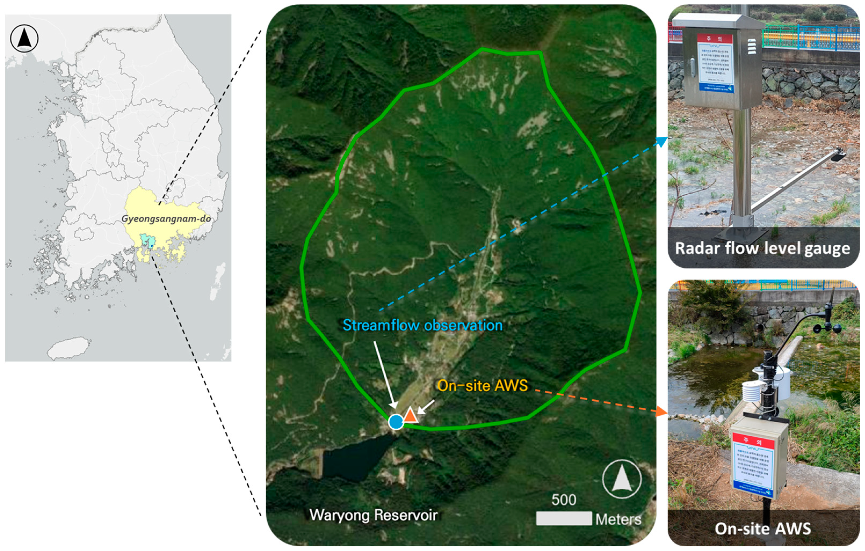
Figure 1. Study site located in southern Gyeongsangnam-do, with observation spots with one radar flow level gauge and one AWS.
Hydrology 11 00162 g001
Figure 2. Screen interface of Cell2Flood model showing its graphical user interface and auto-calibration module.
Hydrology 11 00162 g002
Figure 3. Spatial input data for Cell2Flood, which were converted into an ASCII file with 500 m spatial resolution as the input data for Cell2Flood.
Hydrology 11 00162 g003
Figure 4. Geographical distribution of rain gauge (ASOS and AWS) stations around the study site.
Hydrology 11 00162 g004
Figure 5. Comparison of accumulated rainfall for each rainfall input by events.
Hydrology 11 00162 g005
Figure 6. Change in accumulated rainfall in 1 h intervals of each event by rainfall inputs.
Hydrology 11 00162 g006
Figure 7. Comparison of 1 h maximum rainfall intensity for each rainfall input by events.
Hydrology 11 00162 g007
Figure 8. Comparison of the spatial distribution of 10-min accumulated rainfall for each rainfall input across different events. Event (I) 2023-06-27 22:30, (II) 2023-08-10 07:10, and (III) 2024-06-29 19:00, respectively, and (ac) corresponding to R-ASOS, R-AWS, R-RADAR.
Hydrology 11 00162 g008
Figure 9. Results of rainfall–runoff simulations for Event I by rainfall inputs.
Hydrology 11 00162 g009aHydrology 11 00162 g009b
Figure 10. Results of rainfall–runoff simulations for Event II by rainfall inputs.
Hydrology 11 00162 g010aHydrology 11 00162 g010b
Figure 11. Results of rainfall–runoff simulations for Event III by rainfall inputs.
Hydrology 11 00162 g011aHydrology 11 00162 g011b
Figure 12. Results of rainfall–runoff simulations with the input-specific calibrated parameters for P-ASOS.
Hydrology 11 00162 g012
Figure 13. Results of rainfall–runoff simulations with the input-specific calibrated parameters for P-AWS.
Hydrology 11 00162 g013
Figure 14. Results of rainfall–runoff simulations with the input-specific calibrated parameters for R-ASOS.
Hydrology 11 00162 g014
Figure 15. Results of rainfall–runoff simulations with the input-specific calibrated parameters for R-AWS.
Hydrology 11 00162 g015
Figure 16. Results of rainfall–runoff simulations with the input-specific calibrated parameters for R-RADAR.
Hydrology 11 00162 g016
Table 1. Summary of the selected rainfall events.
EventsStarting TimeEnding TimeDuration
(h)
Accumulated Rainfall
(mm)
Average Rainfall Intensity
(mm/h)
I2023.06.27. 18:002023.06.28. 10:0016:00143.410.2
II2023.08.09. 17:002023.08.10. 13:0020:00190.411.3
III2024.06.29. 11:002024.06.29. 22:0011:0074.66.2
Table 2. Comparison between the on-site observed (P-OA) and different rainfall inputs.
EventsErrorsP-ASOS (1)P-AWS (2)R-ASOS (3)R-AWS (4)R-RADAR (5)
IRMSE (mm)3.003.332.052.882.60
NSE−0.24−0.530.42-0.140.06
Pearson’s r0.470.270.680.290.35
R-square0.220.070.460.090.12
P-bias (%)−0.49−3.9116.20−4.55−41.63
MAE (mm)1.521.631.121.621.83
NPE0.240.35−0.60−0.22−0.72
PTE (min)0.0070.00−10.0060.00−30.00
IIRMSE (mm)1.041.311.060.961.56
NSE0.420.070.400.50−0.31
Pearson’s r0.750.500.750.760.36
R-square0.570.250.560.580.13
P-bias (%)34.6138.0830.8925.11−58.61
MAE (mm)1.081.721.120.932.43
NPE−0.27−0.29−0.47−0.31−0.48
PTE (min)−40.0010.0010.000.0040.00
IIIRMSE (mm)0.962.191.541.071.74
NSE0.63−0.910.050.54−0.20
Pearson’s r0.840.290.340.780.41
R-square0.700.090.120.610.17
P-bias (%)28.95−12.0623.1623.44−80.82
MAE (mm)0.914.802.391.153.02
NPE−0.50−0.03−0.55−0.62−0.65
PTE (min)20.0010.0010.000.00−70.00
(1) P-ASOS: Rainfall at ASOS Jinju (192). (2) P-AWS: Rainfall at AWS Samcheonpo (907). (3) R-ASOS: Area-averaged rainfall interpolated from ASOS stations. (4) R-AWS: Area-averaged rainfall interpolated from ASOS as well as AWS stations. (5) R-RADAR: Area-averaged rainfall from composite HSR by KMA. Bold values indicate the least errors among the other rainfall inputs.
Table 3. Parameters of Cell2Flood calibrated using the on-site observation records, P-OA, for the study basin.
ParametersDescriptionValue
nratioRatio factor for streamflow adjustment based on Manning’s roughness coefficient, which primarily governs surface discharge by accounting for surface roughness and flow resistance25.0
AratioRatio factor for classifying the stream area in a cell, affecting channel flow and travel time on the surface layer26.0
DratioRatio factor for the effective soil depth of each cell, affecting soil saturation in the interflow layer0.4
KratioRatio factor for the steady infiltration rate of each cell, affecting soil moisture on the interflow layer 3.0
GWleakGroundwater leakage rate accounting for surface flow losses0.1
Table 4. Initial conditions for each event based on the on-site rainfall (P-OA).
ParametersUnitDescriptionEvents
IIIIII
SWini%Initial soil moisture45.0100.081.0
GWini%Initial groundwater level based on the surface elevation95.095.095.0
Table 5. Comparison of simulated peak discharge and time-to-peak across rainfall inputs by event.
ItemsObservationP-OAP-ASOSP-AWSR-ASOSR-AWSR-Radar
Event I (2023-06-27 18:00~06-28 10:00)
Peak discharge (m3/s)4.284.6213.753.732.167.234.41
Time-to-peak06-27
23:50
06-27
23:58
06-27
23:55
06-28
01:10
06-28
01:22
06-28
01:13
06-28
05:00
Event II (2023-08-09 17:00~08-10 13:00)
Peak discharge (m3/s)9.198.371.52.362.253.284.67
Time-to-peak08-10
08:20
08-10
08:26
08-10
09:49
08-10
10:12
08-10
08:42
08-10
08:50
08-10
12:04
Event III (2024-06-29 11:00~06-29 22:00)
Peak discharge (m3/s)0.790.750.453.580.470.544.48
Time-to-peak06-29
20:30
06-29
20:50
06-29
20:04
06-29
19:50
06-29
19:40
06-29
20:10
06-29
20:10
Bold values indicate the least discrepancy with the observations except P-OA.
Table 6. Performance of the simulated runoff discharge with the on-site calibrated parameters across different rainfall inputs.
EventsErrorsP-OAP-ASOSP-AWSR-ASOSR-AWSR-RADAR
IRMSE (m3/s)1.603.121.472.021.750.86
NSE−0.26−3.81−0.06−1.01−0.510.63
R-square0.410.270.490.410.390.73
P-bias (%)48.471.9647.2675.2627.8313.16
MAE (m3/s)1.222.171.121.681.360.60
NPE0.082.21−0.13−0.500.690.03
PTE (min)2.0025.00−70.00−82.00−73.00−300.00
IIRMSE (m3/s)1.633.643.283.312.853.06
NSE0.750.850.870.890.900.81
R-square0.840.910.840.940.860.04
P-bias (%)32.4689.8287.4273.5272.93−98.78
MAE (m3/s)0.941.451.421.221.192.71
NPE−0.09−0.89−0.80−0.76−0.640.52
PTE (min)−6.00−89.00−112.0022.00−30.00−224.00
IIIRMSE (m3/s)0.070.171.140.130.112.13
NSE0.920.50−22.550.690.80−81.24
R-square0.940.880.800.840.960.75
P-bias (%)−3.0959.52−304.1441.4341.64−825.36
MAE (m3/s)0.040.110.610.090.081.51
NPE−0.05−0.433.54−0.410.324.66
PTE (min)−20.0026.0040.0050.0020.0020.00
Bold values indicate the least errors with the observations.
Table 7. Parameters of Cell2Flood calibrated based on each rainfall input.
ParametersP-ASOSP-AWSR-ASOSR-AWSR-RADAR
nratio1.06.00.55.01.0
Aratio1.01.01.05.010.0
Dratio1.90.53.22.52.5
Kratio3.54.41.51.23.5
GWleak0.10.10.10.10.1
Table 8. Performance of the simulated runoff with rainfall input-specific calibrated parameters across different rainfall inputs.
EventsErrorsP-ASOSP-AWSR-ASOSR-AWSR-RADAR
IRMSE (m3/s)0.701.991.580.810.75
NSE0.76−0.97−0.240.680.73
R-square0.850.150.430.770.74
P-bias (%)14.7447.0350.7815.097.62
MAE (m3/s)0.501.571.200.570.66
NPE0.040.12−0.010.040.00
PTE (min)17.0017.00−73.00−19.00−99.00
IIRMSE (m3/s)0.911.371.081.601.66
NSE0.920.820.880.750.73
R-square0.920.890.900.820.87
P-bias (%)1.425.6915.8516.95−29.03
MAE (m3/s)0.600.880.631.001.08
NPE0.030.130.000.140.10
PTE (min)−79.009.0011.00−29.00−219.00
IIIRMSE (m3/s)0.090.180.100.110.07
NSE0.860.390.800.790.91
R-square0.920.590.900.870.95
P-bias (%)19.8941.310.1714.839.68
MAE (m3/s)0.060.120.060.080.05
NPE0.030.100.110.10−0.09
PTE (min)5.00−31.0037.00−19.008.86
Bold vales indicate the least errors with the observations.
Disclaimer/Publisher’s Note: The statements, opinions and data contained in all publications are solely those of the individual author(s) and contributor(s) and not of MDPI and/or the editor(s). MDPI and/or the editor(s) disclaim responsibility for any injury to people or property resulting from any ideas, methods, instructions or products referred to in the content.