Article

Performance Evaluation of Gradient Descent Optimizers in Estuarine Turbidity Estimation with Multilayer Perceptron and Sentinel-2 Imagery

by
Naledzani Ndou
1,* and
Nolonwabo Nontongana
2
1
Department of GIS and Remote Sensing, University of Fort Hare, P/Bag X1314, Alice 5700, South Africa
2
Department of Biochemistry and Microbiology, University of Fort Hare, P/Bag X1314, Alice 5700, South Africa
*
Author to whom correspondence should be addressed.
Hydrology 2024, 11(10), 164; https://doi.org/10.3390/hydrology11100164
Submission received: 29 August 2024 / Revised: 18 September 2024 / Accepted: 30 September 2024 / Published: 3 October 2024
(This article belongs to the Section Marine Environment and Hydrology Interactions)

Abstract

:
Accurate monitoring of estuarine turbidity patterns is important for maintaining aquatic ecological balance and devising informed estuarine management strategies. This study aimed to enhance the prediction of estuarine turbidity patterns by enhancing the performance of the multilayer perceptron (MLP) network through the introduction of stochastic gradient descent (SGD) and momentum gradient descent (MGD). To achieve this, Sentinel-2 multispectral imagery was used as the base on which spectral radiance properties of estuarine waters were analyzed against field-measured turbidity data. In this case, blue, green, red, red edge, near-infrared and shortwave spectral bands were selected for empirical relationship establishment and model development. Inverse distance weighting (IDW) spatial interpolation was employed to produce raster-based turbidity data of the study area based on field-measured data. The IDW image was subsequently binarized using the bi-level thresholding technique to produce a Boolean image. Prior to empirical model development, the selected spectral bands were calibrated to turbidity using multilayer perceptron neural network trained with the sigmoid activation function with stochastic gradient descent (SGD) optimizer and then with sigmoid activation function with momentum gradient descent optimizer. The Boolean image produced from IDW interpolation was used as the base on which the sigmoid activation function calibrated image pixels to turbidity. Empirical models were developed using selected uncalibrated and calibrated spectral bands. The results from all the selected models generally revealed a stronger relationship of the red spectral channel with measured turbidity than with other selected spectral bands. Among these models, the MLP trained with MGD produced a coefficient of determination (r2) value of 0.92 on the red spectral band, followed by the MLP with MGD on the green spectral band and SGD on the red spectral band, with r2 values of 0.75 and 0.72, respectively. The relative error of mean (REM) and r2 results revealed accurate turbidity prediction by the sigmoid with MGD compared to other models. Overall, this study demonstrated the prospect of deploying ensemble techniques on Sentinel-2 multispectral bands in spatially constructing missing estuarine turbidity data.

1. Introduction

Turbidity is considered a significant indicator of estuarine water quality [1], and its assessment is important for estuarine water management and aquatic ecosystem conservation. Turbidity, measured in nephelometric turbidity units (NTU), is defined as the amount of light scattered or blocked by particles suspended in water [2]. It is typically composed of nutrients, bacteria, algae, dissolved colored organic compounds, and other organic and inorganic matter [3]. High concentration of turbidity is known to inhibit the depth at which light can reach [4]. In the Great Fish Estuary, turbidity has become a common phenomenon due to the water exchange between the ocean and the river. Exacerbating this situation are various anthropogenic activities, such as agricultural practices, the removal of riparian vegetation, and raw sewage from Cradock Town, South Africa, discharged into the Great Fish River without being treated. This has subsequently compromised the water quality and ecological functioning of the estuary. Therefore, knowledge regarding spatial distribution and plume dynamics of turbidity in these environments is critical for effective estuarine resource management [5]. Data on turbidity are conventionally obtained through field-based sampling techniques, which are labor-intensive, time-consuming, and costly. Moreover, field-based data are acquired from individual sampled locations, posing questions about missing data at unsampled locations. To this end, spatial interpolation approaches have been extensively deployed to account for missing data at unsampled locations [6,7]. Kriging and inverse distance weighting (IDW) techniques are commonly used to generate turbidity data based on the linear weighting of surrounding measured values [8,9]. However, there is no single technique which alone is capable of accurately predicting dynamic variables such as estuarine turbidity.
Advances in remote sensing technology offer a convenient and spatially explicit opportunity to enhance estuarine turbidity monitoring [10]. Multispectral sensors have consistently and efficiently been deployed to track estuarine turbidity through analysis of spectral radiance properties of estuarine waters [11], guided by the notion that turbid waters tend to inherit optical properties from suspended particles. These sensors are still considered vital tools for turbidity mapping in many developing countries due to the free access to their data. Therefore, satellite multispectral data from sensors such as Sentinel-2 [12,13], Landsat generations [14,15], Aster [16], and MODIS [17] have been widely used to monitor turbidity. Among these images, Sentinel-2 imagery is recommended for turbidity estimation due to its higher spatial resolution of 10 m. As such, individual spectral bands and indices generated from the combination of spectral bands, such as the Normalize Difference Turbidity Index (NDTI) and the turbidity index [1], have been used to predict turbidity patterns. However, characterizing estuarine turbidity with these sensors is challenging because estuarine waters are dynamic in nature, and they require sensors with high signal-to-noise ratios [12]. Moreover, individual spectral bands and spectral indices serve only as proxies for turbidity, as they do not provide the actual level of turbidity concentration. As such, these spectral bands and indices, in conjunction with field-measured turbidity data, are used to predict turbidity concentrations through either empirical or analytical approaches [18]. While analytical methods rely on radiative transfer equations to derive the inherent optical properties of dynamic waters [19], empirical methods optically retrieve waters by establishing relationships between water reflectance and field-measured waters. However, accurate prediction of estuarine turbidity patterns using either analytical or empirical approaches remains a challenging task, due to the dynamic nature of estuarine waters [20]. Empirical approaches require large data samples with good spread [21] and are valid for the areas they were established in. On the other hand, analytical approaches are prone to atmospheric correction errors when applied to satellite imagery [19]. As such, a more sophisticated, data-driven, and self-adaptive approach is required to exploit spectral information from satellite imagery [22].
Evidently, the applications of artificial neural networks (ANNs) to address limitations associated with analytical and/or empirical models have extensively been acknowledged [23,24]. The multilayer perceptron neural network (MLP), in particular, has demonstrated the ability to learn dynamic estuarine processes [25,26], taking advantage of its backpropagation architecture, which facilitates back-forward learning [27]. Trained with a sigmoid activation function, the MLP can learn dynamic, non-linear, complex processes such as estuarine turbidity [28]. From a multispectral image perspective, the outcome of the MLP learning process is the probability of image pixels belonging to turbidity, instead of pixels directly becoming members of the turbidity class. Therefore, all pixels in the image are reconfigured to represent turbidity only. Several studies have recommended the application of the MLP in turbidity prediction [29,30,31]. However, it is worth noting that any traditional deep learning approach alone does not have the ability to learn rapidly changing patterns [32], such as estuarine turbidity. The MLP, in particular, is symmetrical and does not perform well with highly biased distributions [29]. The performance of the MLP is influenced by its learning rate, which determines the values of weights and biases that reduce the prediction error with training data [33]. Moreover, the influence of initial weights in the MLP has not been effectively addressed, as they play a major role in determining its performance [34,35]. The backpropagation algorithm has multiple drawbacks that affect convergence in the MLP learning process, such as terminating the learning process in local optima. This has led to the MLP becoming more reliant on the initial values of hyperparameters [36].
If parameters such as network topology, initial weights, biases, learning rate value, and activation function are not appropriately selected, it can result in a slow convergence rate, network error, or failure when calibrating image pixels to turbidity when training the MLP using the sigmoid cross-entropy function [37,38]. As such, the MLP approach is not suitable for learning dynamic processes in unknown environments alone [39]. Several performance optimizers were proposed to enhance MLP performance by accurately determining the initial weights and these include Kaiming initialization [40], Xavier (Glorot) initialization [41], orthogonal initialization [42] and gradient descent (GD) optimizers [40]. However, the GD algorithm is considered one of the most reliable optimization algorithms [37]. As such, several GD approaches have been proposed to perform error backpropagation processing, i.e., optimizing the learning rate while minimizing the error between the output value computed by the model and the anticipated value [21]. The primary focus in gradient descent is to minimize the error function by adjusting the weights in the network [35]. These GD approaches include stochastic gradient descent (SGD) [43], momentum gradient descent (MGD) [44], Fractional Order Gradient Descent [45], Damped Newton Stochastic Gradient Descent [46], Nesterov accelerated gradient (NAG) [47] and Adaptive Gradient Algorithm (AdaGrad) [48], among others. When specifically used with momentum gradient descent, the MLP learning rate is increased by setting the momentum factor to 0.9, weight decay to 10−4, and the initial learning rate to 0.1 [49]. In this case, the role of the momentum factor in gradient descent is to accelerate the convergence rate of the MLP optimization algorithm [50]. Furthermore, Lee et al. [51] noted that the significant influence of the gradient approaches in enhancing model performance in water quality prediction is frequently not evaluated. Through the literature search, studies that sought to monitor turbidity patterns based on remote sensing approaches have mainly utilized semi-analytic or empirical models based on the relationship between spectral radiance properties of water and field-measured turbidity [52,53,54,55,56]. As such, we noted that studies on enhancing MLP performance through the introduction of SGD and MGD for optimized prediction of estuarine turbidity patterns are lacking. Remote sensing reflectance to field turbidity [57]. In this study, we evaluated two commonly used GD approaches, viz., SGD and MGD, in improving MLP performance for predicting estuarine turbidity patterns. Prior to performance evaluation of SGD and MGD, we evaluated the efficacy of linear regression on uncalibrated spectral bands of Sentinel-2 imagery.

2. Materials and Methods

2.1. Study Area

The Great Fish Estuary is situated in the Ndlambe Local Municipality of the Sarah Baartman District Municipality of the Eastern Cape Province in South Africa. The study area is located between 33°28′13.16″ S; 27°04′55.76″ E and 33°30′22.4″ S; 27°07′58.21″ E absolute locations. It serves as the base for ecosystem functioning of the coastal environment of the Eastern Cape Province of South Africa. This estuary is also used for fishing by the local communities. The estuary is situated within the elevation range of 0 m above sea level (a.s.l.) to 16.16 m a.s.l. Figure 1 shows the location of the study area, with the locations for sampled data highlighted. The Great Fish Estuary in South Africa is no exception regarding water contamination. The principal alarming source of water pollution in this estuary is a large volume of raw, untreated wastewater from the Cradock dysfunctional water treatment plant, which is discharged into the Great Fish River.

2.2. Methods

The sequence of methods and techniques deployed to attain the main objective of this study is presented in Figure 2.

2.3. Data Acquisition

2.3.1. Satellite Data

The Sentinel-2 imagery, acquired with the multispectral instrument (MSI) and having the ID: T35HND_20220630T074619, was downloaded from the European Space Agency (ESA) Sentinel Scientific Data Hub (https://scihub.copernicus.eu/), accessed on 13 August 2022. This satellite imagery was preferred over other cost-free sensors, such as Landsat, due to its reasonably higher spatial resolution of 10 m in its four visible-NIR bands, 20 m in three bands in the red edge and two bands in shortwave infrared (SWIR) [58], 60 m in its coastal aerosol band, SWIR-cirrus band, and water vapor band, and a 12-bit radiometric resolution. The image used for this study was acquired on 30 June 2022 at 07:46:19 South African local time, with the date and time selected based on cloudless conditions. The empirical relationship between turbidity and spectral reflectance in the blue [59], green [52], red [60], red edge [61], NIR [62], and SWIR [63] spectral channels justified the selection of these spectral channels from Sentinel-2 imagery for model training. Coastal aerosol, water vapor, and SWIR-cirrus spectral channels were omitted in this study due to their lack of association with turbidity. Table 1 provides detailed characteristics of the Sentinel-2 spectral bands used in this study.

2.3.2. Field Data Collection

A total of 40 surveyed point samples out of 42 surveyed samples were considered for turbidity modeling in this study. A simple random sampling technique was employed to select the sites where measurements were carried out. Upon the successful identification of the survey sites, the absolute location of each sample point was recorded using the Garmin eTrex 22× Handheld GPS®, with 3 m precision. The field survey was conducted on 30 June 2022 to coincide with the estuarine turbidity data collection period and the Sentinel-2 satellite overpass. The field data were collected from 8h00 to 11h00 local time. The collection of field data during this time was to ensure it was as close to the MSI scanning time as possible. A canoe was used to access sites of deep water. At random pattern, turbidity data were measured near the water’s surface (i.e., at most 0.05 m) using the HANNA HI9829 portable logging multi-parameter meter. The GPS points were recorded in Microsoft Excel and saved as a “.csv” file. This file was imported into the TerrSet software package and converted to a vector GIS point layer. The acquired dataset was partitioned into two sets; i.e., 28 points (70%) of the dataset served in model training, and 12 points (30%) in model validation. However, all the surveyed field sample points were used in the spatial interpolation of turbidity.

2.4. Pre-Processing of Sentinel-2 Imagery

The acquired Sentinel-2 imagery was received already geo-rectified to the Universal Transverse Mercator (UTM) coordinate system, based on the World Geodetic System of 1984 datum (WGS-84), 36° South grid reference. This georeferencing system facilitated the successful position adjustment of the Sentinel-2 imagery in line with its ground position. However, the downloaded image scene extended beyond the boundary of the estuary under investigation. As such, only the portion of the imagery falling within the estuarine boundary was extracted in ArcMap 10.8 GIS software package, using the estuarine boundary shapefile as a mask feature. The Sentinel-2 imagery used in this study was received in Level 1C, having already been radiometrically corrected, with its radiance (L) values ranging from 0 to 1. The Sentinel-2 sensor achieved this by employing geographical locations for imagery referencing [64]. Prior to model development and validation, outliers were removed from the field datasets, to minimize bias in the prediction of turbidity. The outliers in this study were two turbidity records whose values were extremely high, such that their inclusion would move the mean value closer to the highest turbidity value when they were not included.

2.5. Estuarine Water Body Demarcation

Prior to the extraction of pixel values from selected spectral bands, the estuarine water body requires to be masked to ensure that the experimental site contained only water pixels [65]. The estuarine water body was demarcated on satellite imagery by employing the Modified Normalized Difference Water Index (MNDWI) based on Equation (1):
M N D W I = ρ G + ρ S W I R 1 ρ G + ρ S W I R 1
where ρ is the radiance value of the specified spectral channel; G is the green channel; and S W I R 1 is the first shortwave-infrared channel of the Sentinel-2 sensor.
The selection of this spectral index was based on its ability to suppress reflectance from built-up features by deploying the shortwave infrared band instead of the near-infrared, commonly used in the normalized difference water index (NDWI) [66].

2.6. Analyzing Spatial Variability in Water Radiance Values across Selected Spectral Bands

A total of 300 pixels were randomly collected to obtain the spectral radiance sample that served as input for model training. Prior to model training, Levene’s k-comparison of variance statistical test was used to determine spatial variability in the spectral radiance properties of estuarine waters across selected spectral channels of Sentinel-2 imagery. Levene’s test was computed using Equation (2), adopted from Pare’ et al. [67]:
W = N k i = 1 k N i Z ¯ i . Z ¯ . . 2 k 1 i = 1 k j = 1 N i Z i j Z ¯ i . 2
where Z i j = | Y i j Ȳ i | , with Yij the value of Y for the j-th observation of the i-th subgroup; Ȳi is the mean of the i-th subgroup; Z ¯ i is the mean of the group Z i j ; and Z ¯ is the overall mean of the Z i j .
Subsequently, the mean radiance values for selected spectral channels were used to plot the spectral reflectance behavior of estuarine waters.

2.7. Spatial Pattern Analysis of Turbidity

Spatial variability in the field-measured turbidity was established using the Bayesian one-sample t-test. Under a supposition that sample X ( n ) = { X 1 ,   X 2 ,   ,   X n } of size n is randomly distributed, and each data point is sampled from a location in estuarine waters, the Bayesian one-sample t-test computed the pattern by applying Equation (3), adopted from Emmert-Streib and Dehmer [68]:
X ̄ ~ N µ , σ n
where { X 1 ,   ,   X n } are random samples with μ and σ2, which follow a normal distribution.
Subsequently, the turbidity pattern was constructed using IDW interpolation on the field-measured data. This technique functions based on the notion that “values closer together tend to be more similar than those further apart” [69]. To spatially construct missing values, the algorithm utilizes two or more of the closest measured values [70]. As such, a weighted sum was applied across measured values to determine the value of the interpolated region, based on Euclidean distance by employing Equation (4), adopted from Chin et al. [69]:
Z 0 = i = 1 S Z i 1 d i k   i = 1 S 1 d i k
where Z 0 is the estimated value at the unsampled location; Z i is the measured value; di is the distance between the estimated and observed locations; s is the number of measured sampling points within the neighborhood; and k is the parameter containing the exponential value, which defines the degree to which the value is reduced as the distance increases.

2.8. Binarization of IDW Image and Thresholding of Turbidity Level

The raster-based turbidity image acquired through IDW was used as a training mask in the MLP model development. The training sites were demarcated using the bi-level thresholding technique, such that:
T s i t e = 1   i f   T u r b i d i t y T 0 ,   o t h e r w i s e    
where Tsite is the training site; and T is the threshold, equal to or above which the model was trained. This was set to 50.0 NTU according to Kopsachilis et al. [71]. The motive behind training the model on a binarized IDW map was due to the fact that the interpolated turbidity contained the actual field-measured turbidity.

2.9. Model Training

A point shapefile containing the locations and values of turbidity was overlaid on each selected spectral band and NDTI in the ArcGIS 10.8 GIS platform. The radiance and index values were extracted from the selected spectral bands and NDTI, respectively, using the “Extract Multi Values To Point” module. The extracted spectral bands and spectral index were used in model training. The following models were tested for their efficacy in spatially constructing missing turbidity data.

2.9.1. Linear Regression

The relationship between the spectral radiance values and field-measured turbidity was established using linear regression analysis, based on Equation (6), adopted from Hossain et al. [14]:
y = m x + b  
where Y is the dependent variable; m is the slope; x is the explanatory variable; and b is the intercept of Y.
The nature and degree of the relationship were evaluated by interpreting the regression coefficient values and least-squared regression (r2).

2.9.2. Training MLP with Sigmoid Activation Function and SGD

Prior to the data split into training and validation sets, the data were pre-randomized to minimize selection bias associated with training and validation data. During the training process, each sample (pixel values extracted from each selected spectral band of Sentinel-2 imagery) was fed into the respective neurons of the input layer of the MLP algorithm. Each receiving neuron in the input layer then weighted signals from all the neurons to which it is connected in the preceding layer. The weight of the signals received by a single neuron was determined by employing Equation (7), adopted from Fierro et al. [72]:
n e t j = i 1 m x i w i j + o j
where N e t j is the total weight of the j-th neuron for the input samples received from the preceding layer with n neurons; x i is the input value to the i-th node of the input layer; and w i j is the weight between the i-th node of the input layer and node j of the hidden layer.
Assuming w m represents the value after iteration m of a weight w, which can be either a hidden neuron weight wij or an output neuron weight w j k , w m was determined using Equation (8), according to Shimodaira [73]:
w m = w m 1 + w m
where Δ w m is the change in the weight w at the end of iteration m and is obtained by employing Equation (9):
w m = ε × d m  
where ε is the parameter controlling the proportion by which the weights are changed. However, dm is obtained by applying Equation (10), adopted from Shimodaira [73]:
d m = n = 1 N E w m n  
where E is the cost error; and w m is the parameter at the recurrent step.
Oj is the output from neuron j, expressed using Equation (11):
o j = f n e t j  
where
N e t j is provided in Equation (7).
The sigmoid activation function was used to account for variability over the sampled spectral radiance denoting turbidity by employing a non-linear transformation to optimize turbidity prediction using Equation (12), adopted from Platt [74]:
s x = 1 1 + e x
where s ( x ) denotes the sigmoid activation function, and e ≈ 2.71 is the base of the natural logarithm.
Stochastic gradient descent was introduced into the sigmoid activation function, to optimize MLP performance by minimizing the loss function. The SGD method improved the learning rate by randomly selecting samples based on Equation (13), according to Kaddoura [75]:
J θ i = 1 N y i θ T X i X i
where
J ( θ ) is the gradient descent;
i denotes the individual row of the dataset;
N denotes the number of datasets in the i-th row;
where i is each row of the data set.
The model was continuously trained to compute the gradient and update parameters until the error was less than a threshold, or the number of iterations reached a threshold. The model was trained in the TerrSet Geospatial Monitoring and Modeling software platform. Table 2 provides a summary of learning parameters for the MLP with a sigmoid activation function.
As such, the sigmoid function for each dependent variable was set to saturate at 1.0, to allow the activation function to become increasingly more linear in character.

2.9.3. Training MLP with Sigmoid Activation Function and MGD

The MLP was also trained with the sigmoid activation function (explained in Section 2.9.2) and momentum gradient descent. In this case, the training epochs were also set to 500, at a learning rate of 10−5. Momentum gradient descent was introduced into the MLP algorithm according to Chen et al. [43], such that:
ω i j = η × E ω i j  
where
ω i j is the weight increment along the i-th and j-th nodes;
η is the learning rate;
E ω i j is the weight gradient, according to Chen et al. [43], such that:
ω i j t = η × E ω i j + γ × ω i j t 1
where
γ is the momentum factor; ω is the weight along the gradient; t is the time at which the weight is incremented; and ω i j t 1 is the weight increment at the previous iteration.

2.10. Evaluation of the Model Performance

A total of 12 samples (30%) of the total turbidity data reserved for performance evaluation were saved as .csv and converted to shapefiles. The created point shapefile was then superimposed on the turbidity images predicted by the LR, MLP with SGD, and MLP with MGD algorithms. The pixel values were then extracted to the point shapefile, with a view to determine the nature and degree of their association with the predicted turbidity. The performance of each utilized model was evaluated by employing least-squared regression (r2) using Equation (16), adopted from Yan et al. [76], and the relative error of mean (REM) using Equation (17), adopted from Ndou et al. [77]:
R 2 = 1 i = 1 n x i x i 2 i = 1 n y i y ¯ i 2  
where y i denotes the observed turbidity; y i denotes the mean of the observed turbidity;
R E M = T m e a s u r e d T p r e d i c t e d T m e a s u r e d × 100 %
where T m e a s u r e d is the measured value of turbidity, and T p r e d i c t e d is the predicted value of turbidity.

3. Results

3.1. Spectral Radiance Patterns of Estuarine Turbid Waters

Spectral radiance patterns of estuarine waters were analyzed in this study. In the absence of turbidity in the estuary, water radiance properties are expected to be the same across all parts of the estuary. Figure 3 shows radiance values of estuarine waters across different spectral channels of Sentinel-2 imagery.
Generally, the radiance properties of estuarine waters were noted to vary from one spectral channel to another. From Figure 3, the minimum radiance values of the (a) blue, (b) green, (c) red, (d) red edge 1, (e) red edge 2, (f) red edge 3, (g) NIR, (h) red edge 4, (i) SWIR 1, and (j) SWIR 2 spectral bands were noted to be 0.19, 0.16, 0.13, 0.04, 0.11, 0.11, 0.1, 0.05, 0.0, and 0.0, respectively. Moreover, the maximum radiance values of the same spectral bands were noted to be 0.54, 0.53, 0.53, 0.56, 0.61, 0.61, 0.73, 0.74, 0.5, and 0.38, respectively. From randomly sampled pixels, Levene’s k-comparison of variance statistics for the spectral radiance properties of estuarine waters is presented in Table 3.
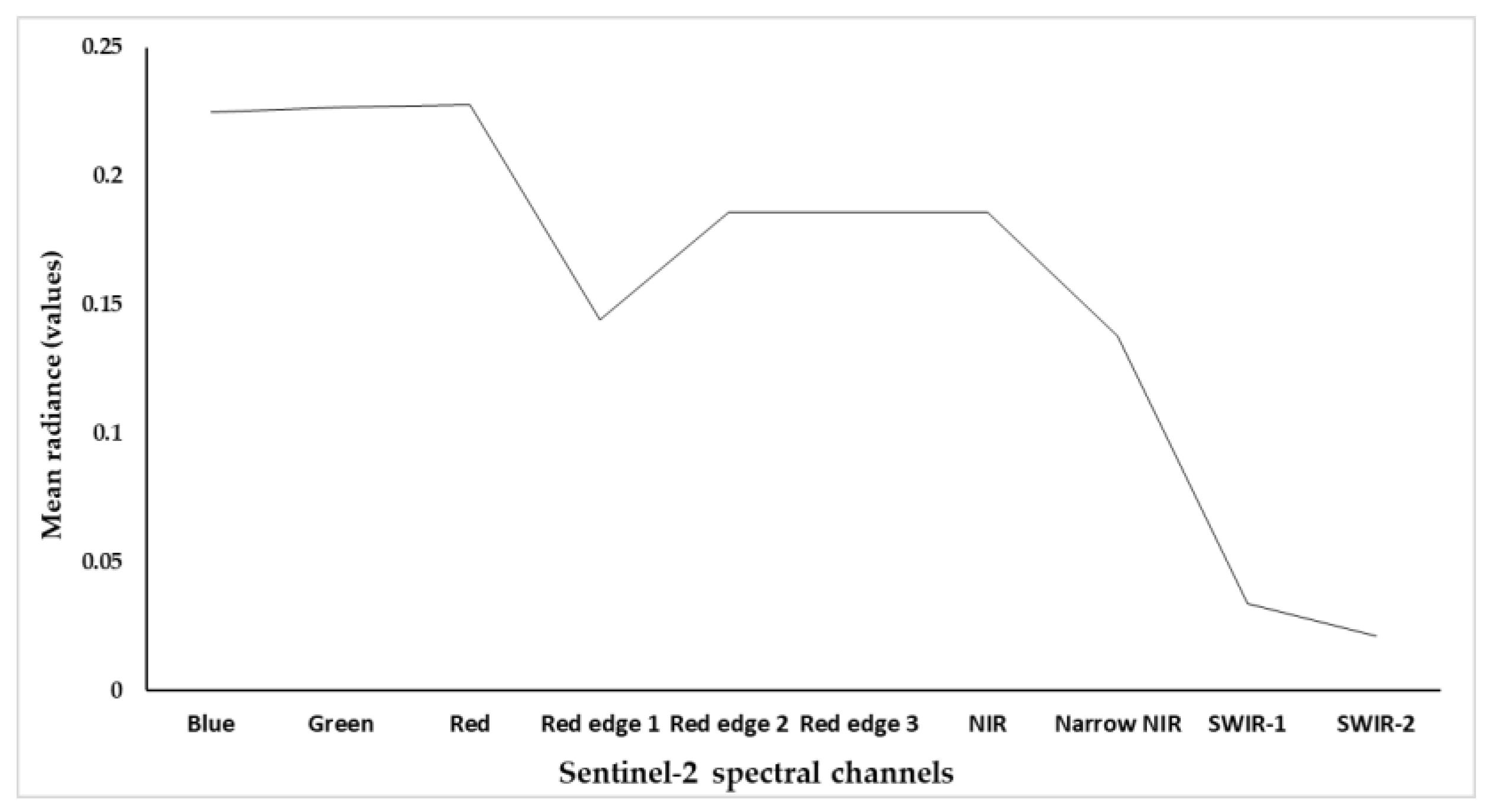
At N of 300, DF of 299, and 0.05 significance alpha (α), the mean radiance properties of waters were found to be 0.225, 0.227, 0.228, 0.144, 0.186, 0.186, 0.186, 0.138, 0.034, and 0.021 for blue, green, red, red edge 1, red edge 2, red edge 3, NIR, red edge 4, SWIR 1, and SWIR 2, respectively. The p-value obtained from Levene’s k-comparison of variance statistics was noted to be below 0.001, which is less than 0.05 significance alpha. By implication, the radiance properties of waters varied across the spectral wavelengths of the Sentinel-2 sensor.

3.2. Mean Radiance Values of Various Sentinel-2 Spectral Channels

Upon the successful analysis of descriptive statistics of water radiance properties, the mean spectral radiance profile for estuarine waters was plotted (Figure 4).
From the mean radiance properties graph, it was apparent that estuarine waters had higher reflectance in the red spectral channel and lower reflectance in the SWIR 2 spectral channel (Table 2).

3.3. Spatial Patterns of Turbidity across the Surveyed Sites

Under a supposition that there is no difference in the measured turbidity levels across the surveyed sites in the estuary, the computed descriptive statistics are presented in Table 4.
At N of 32, DF of 31, and 0.05 significance alpha (α), the mean value, computed from field-based data, for turbidity was noted to be 43.635, with a standard deviation, standard error, t-value, and p-value of 41.279, 8.607, 5.070, and less than 0.001, respectively. As the computed p-value was noted to be less than 0.05 α, the assumption that there are no significant variations in the distribution of turbidity across the surveyed sites does not hold, implying heterogeneity in turbidity concentration.

3.4. Relationship Establishment between Sentinel-2 Spectral Radiance Values and Turbidity Concentration

3.4.1. Linear Regression Model on Uncalibrated Spectral Bands

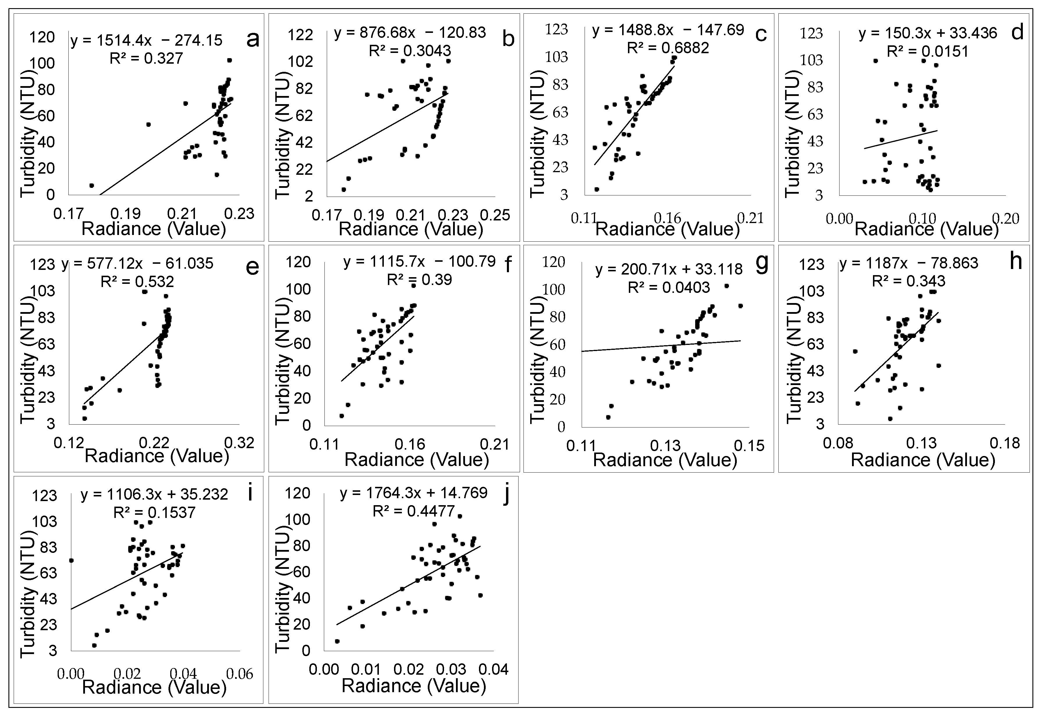
Linear regression analysis was performed to establish the relationship between measured turbidity data and the spectral radiance properties of estuarine waters. Figure 5 presents the nature and degree of the association between turbidity and the radiance properties of waters.
From Figure 5, the linear regression results between water turbidity and uncalibrated spectral radiance data revealed r2 values of 0.33, 0.31, 0.69, 0.02, 0.53, 0.39, 0.04, 0.34, 0.15, and 0.45 for the blue, green, red, red edge 1, red edge 2, red edge 3, NIR, red edge 4, SWIR 1, and SWIR 2, respectively. As such, the red band exhibited a stronger relationship with turbidity concentration than the other spectral bands.

3.4.2. MLP Trained with Sigmoid Calibration Function

Demarcation of Training Sites

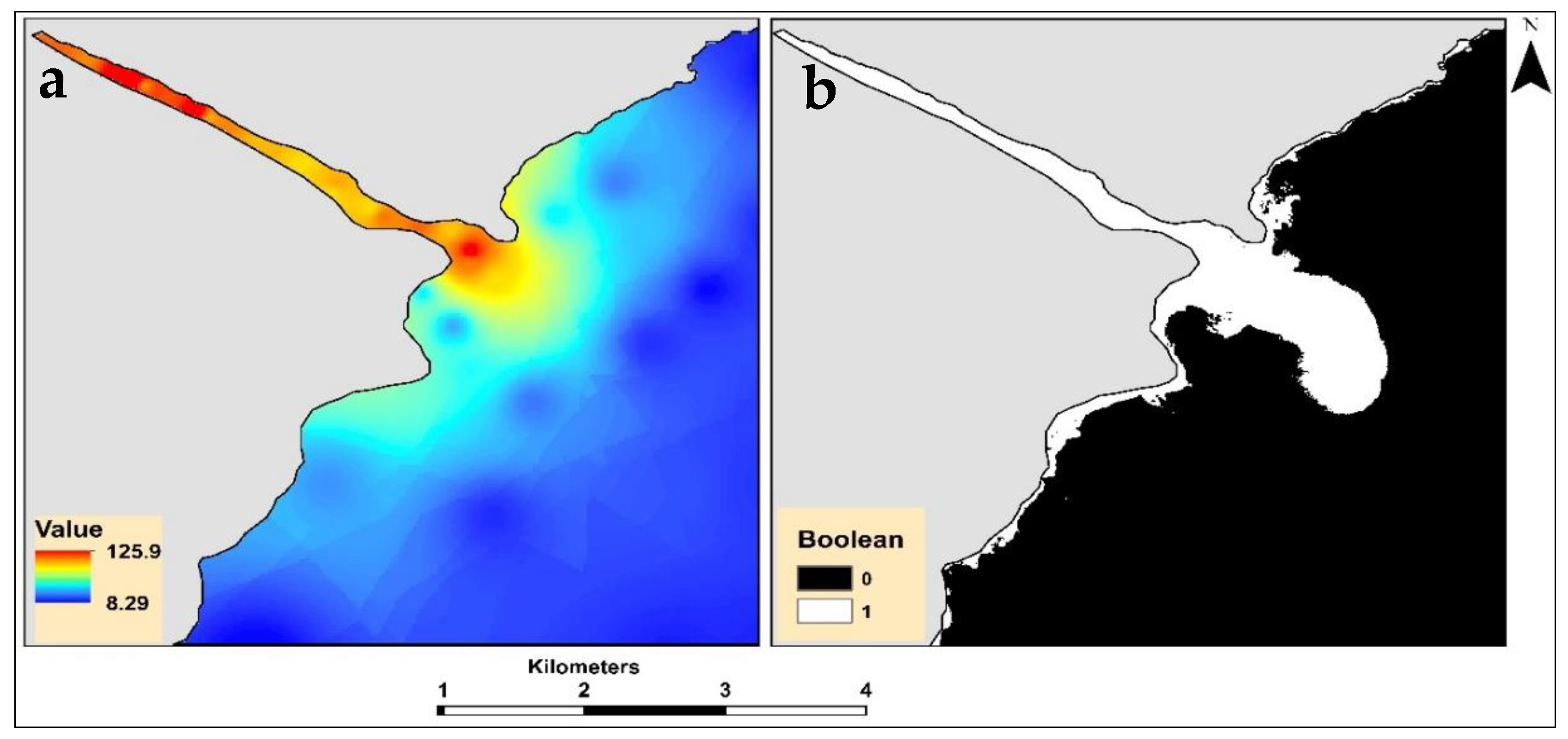
For the artificial neural network method to learn patterns from remotely sensed images, the training site must be demarcated in the image. In this study, the training site was demarcated by binarizing the IDW image. Figure 6 shows the raster image produced by interpolating field-measured turbidity using the IDW interpolation technique and the Boolean image derived from the IDW image.

Linear Regression Model on Spectral Bands Calibrated with Stochastic Gradient Descent

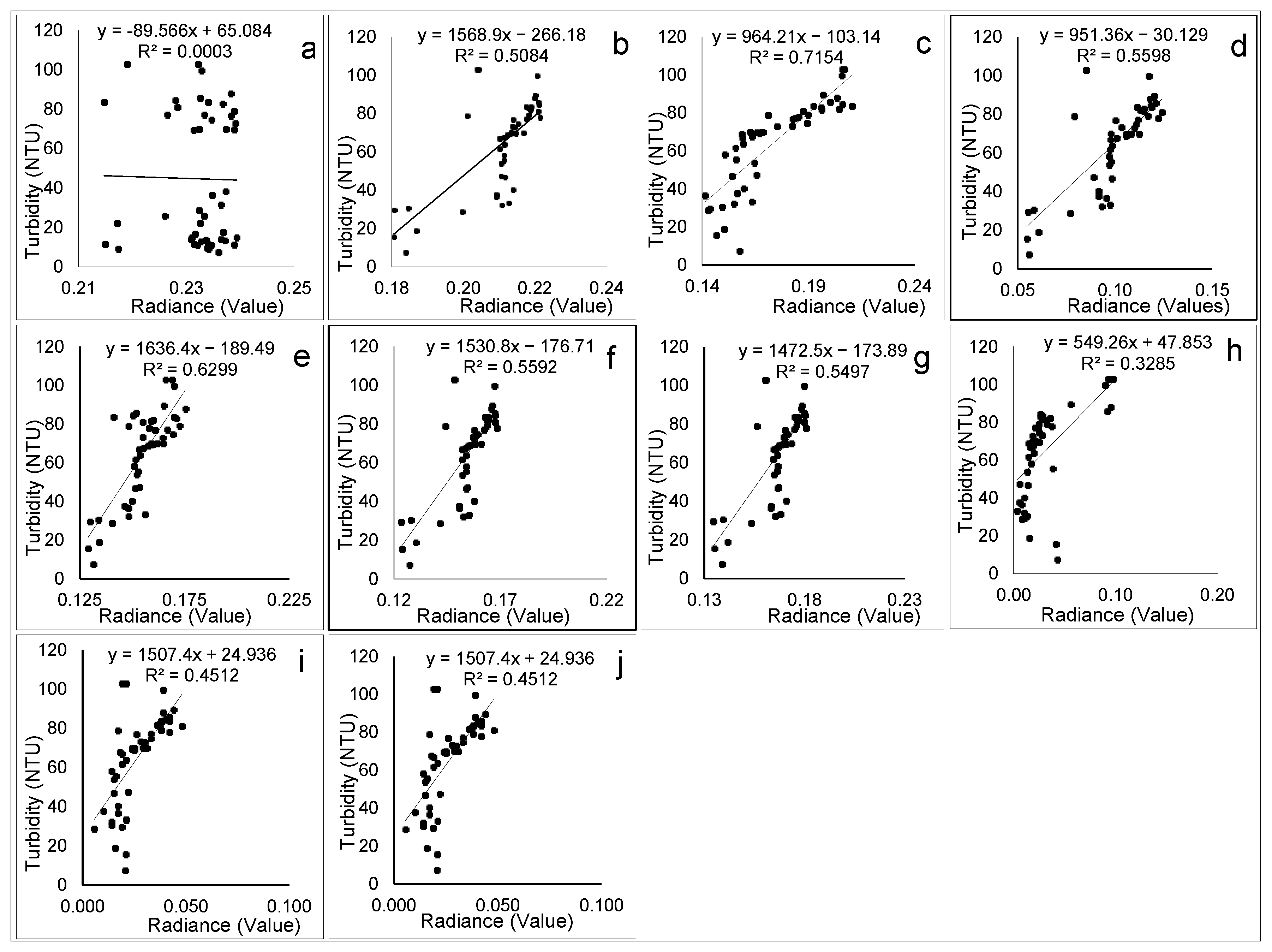
The results obtained from the linear regression model performed on spectral bands calibrated with the sigmoid activation function and stochastic gradient descent are provided in Figure 7.
From Figure 7, the linear regression results between water turbidity and spectral radiance calibrated with the sigmoid function and SGD revealed r2 values of 0.0003, 0.51, 0.72, 0.56, 0.63, 0.56, 0.55, 0.33, 0.45, and 0.38 for blue, green, red, red edge 1, red edge 2, red edge 3, NIR, red edge 4, SWIR 1, and SWIR 2, respectively. As such, the red band calibrated with the sigmoid function and SGD also exhibited a stronger relationship with turbidity concentration than other spectral bands.

Linear Regression Model on Spectral Bands Calibrated with Momentum Gradient Descent

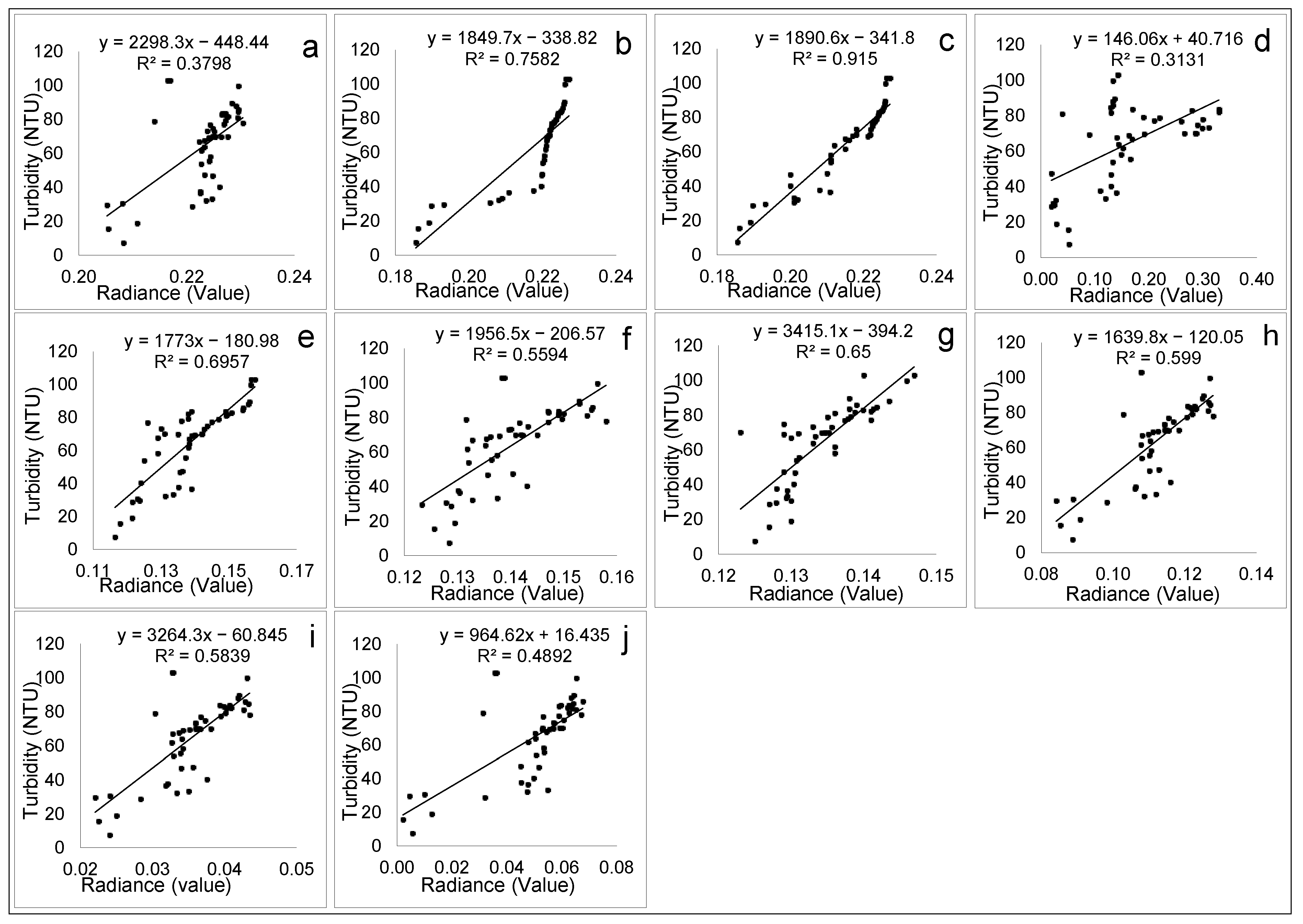
Linear regression analysis results for the relationship between turbidity and spectral bands calibrated with the sigmoid function and MGD are presented in Figure 8.
From Figure 8, the linear regression results between water turbidity and spectral radiance calibrated with the sigmoid function and MGD revealed r2 values of 0.38, 0.76, 0.92, 0.31, 0.69, 0.56, 0.65, 0.6, 0.58, and 0.49 for blue, green, red, red edge 1, red edge 2, red edge 3, NIR, red edge 4, SWIR 1, and SWIR 2, respectively. As such, green and red bands calibrated with the sigmoid function and MGD exhibited a stronger relationship with turbidity concentration than other spectral bands.

3.4.3. Spatial Modeling of Turbidity Concentration

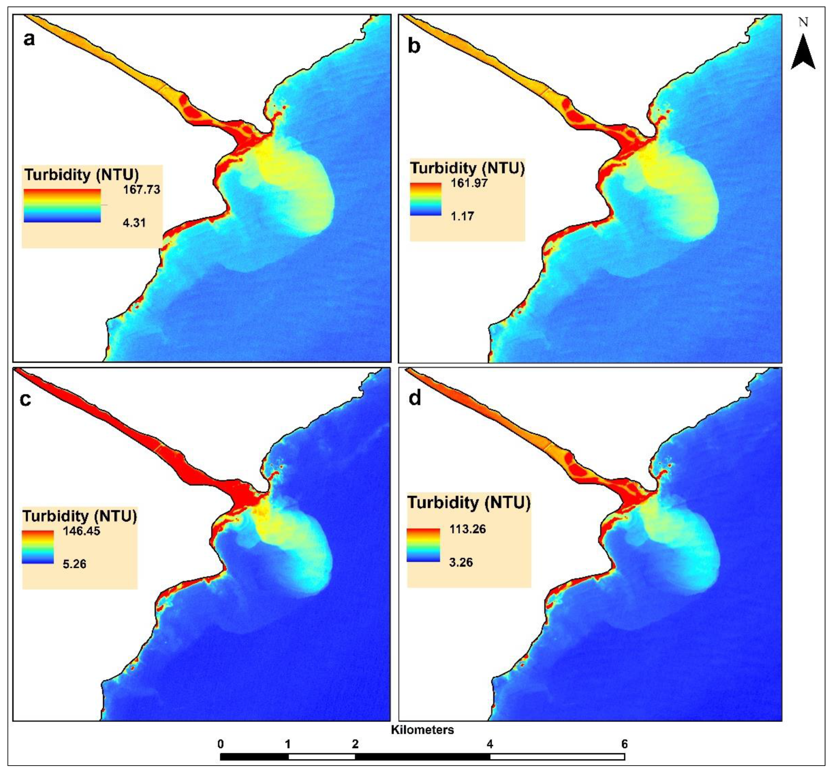
After successfully establishing the relationship between turbidity concentration levels and spectral radiance properties, regression equations for spectral bands that exhibited a strong relationship with turbidity concentration were deployed to model spatial patterns in turbidity levels Figure 9 shows the spatial configuration of turbidity concentration.
From Figure 9, turbidity concentration levels were noted to range from 4.31 NTU to 167.73 NTU, 1.17 NTU to 161.97 NTU, 5.26 NTU to 146.45 NTU, and 3.26 NTU to 113.26 NTU, as modeled with linear regression on the red band, linear regression on the red band calibrated with the sigmoid function and SGD, linear regression on the green band calibrated with the sigmoid function and MGD, and linear regression on the red band calibrated with the sigmoid function and MGD, respectively.

3.4.4. Performance Evaluation of the Models Deployed

R-Squared Results

Figure 10 shows the performance evaluation of the models deployed to estimate spatial patterns in turbidity concentration in the study area.
Based on Figure 10, the established empirical models provided reasonably accurate spatial predictions of turbidity in the study area. However, the linear regression model generated from the red spectral band calibrated with the sigmoid function and MGD showed higher accuracy, with an r2 value of 7.2, than other deployed models (Figure 10d).

3.5. REM Results

Table 5 presents the REM results for the performance evaluation of the models deployed in this study.
Generally, all the deployed models were noted to have overestimated turbidity concentration in the study area. However, turbidity values predicted by the sigmoid function and MGD on the red band showed smaller deviation from the measured turbidity data compared to other deployed models. These findings support the model performance evaluation results obtained by the R-squared model in this study.

4. Discussion

Monitoring spatial patterns in estuarine turbidity is crucial for effectively managing estuarine resources and functionality. However, field-based methods alone do not present a practical approach for full comprehension of spatial patterns in turbidity [61]. As such, acquiring the spatial distribution of water turbidity using remote sensing techniques is deemed a time-efficient, cost-effective, and practical approach, since it presents the overall state of turbidity levels in a water body [1]. This study aimed to evaluate the performance of two gradient descent algorithms in optimizing estuarine turbidity prediction based on MLP and remotely sensed data. Li et al. [12] noted that, even though various statistical and machine learning regression methods have been shown to be capable of predicting turbidity patterns, it is important to evaluate their effectiveness in a comparative manner. For this purpose, Sentinel-2 imagery was used as the base from which spectral radiance properties of turbidity were obtained. The selection of this satellite imagery was informed by its reasonably higher spatial resolution of 10 m and spectral bands sensitive to turbidity. Ma et al. [55] noted that Sentinel-2 imagery has presented a promising base for assessing water turbidity. Other studies have also acknowledged the importance of Sentinel-2 imagery in turbidity monitoring [22,78,79]. However, it must be worth noting that the accuracy of the remote sensing approach alone in studying dynamic processes such as estuarine water turbidity remains questionable. This is because several optically active water constituents that do not have any association may have the same spectral reflectance properties. For this reason, several studies have noted the need to advance existing models for optimizing turbidity estimation using remotely sensed data [10,80,81]. To this end, the integration of remote sensing data and several machine learning algorithms has been recommended as a way to advance turbidity estimation [22,82,83].
Machine learning-based regression approaches have become common techniques in turbidity mapping due to their ability to minimize the impact of data outliers [84,85]. However, when these models are employed without incorporating an appropriate activation function, the envisaged results may not be achieved. As such, deep learning architectures may end up operating in a manner similar to traditional linear regression models. For this reason, non-linear activation functions are preferred in deep neural network architectures [86]. In this study, the MLP algorithm was deployed due to its reliance on the sigmoidal activation function, which has the ability to handle linearly inseparable data [86] during its backpropagation learning. The performance of the sigmoid activation function in training MLP is determined by the desired conditions for convergence speed and error minimization. Although the MLP approach has shown the ability to overcome these issues, the interactions between water constituents and solar radiation are quite complex and present a challenge for this technique. This approach not only exhibits limitations when faced with changing or incremental data regimes but also suffers from catastrophic forgetting [32], as a result of rapidly changing patterns. Yan et al. [87] suggest using the gradient technique to address the limitations of the traditional MLP approach. In this case, the gradient descent is computed using backpropagation on data at different iteration stages [88]. However, minimizing a cost function in a high-dimensional space is intricate for optimizers such as classical gradient descent (GD) [89]. In this study, SGD and MGD optimizers were introduced into the MLP algorithm to discover model parameters that conform to the best predicted actual output. The SGD optimizer demonstrated the ability to overcome limitations associated with classical GD. As the SGD approaches a local optimum, the parameters may oscillate back and forth around the optimum position [90]. From the SGD perspective, global convergence analysis remains crucial in determining the necessity of local analyses, complexity analyses, or saddle point analyses [91]. It is widely recognized that incorporating momentum into an optimization algorithm is necessary for effectively training a large-scale deep network [92]. Including a momentum term m in traditional stochastic gradient descent can speed up learning in relevant directions and minimize oscillations during training by decelerating in lateral dimensions with inconsistent gradients [89]. Sun et al. [46] noted that the MGD optimizer shows no sensitivity to deep learning architectures and hyperparameters. MGD operates by modifying the SGD to speed up convergence and minimize oscillation [92], thereby minimizing noise from stochastic gradients in the early stages [93]. Based on empirical evidence, Sutskever et al. [94] noted that architectures trained with momentum have better performance compared to those trained without it.
Selecting suitable spectral channels for spatial modeling and predicting water turbidity remains a challenge [95]. This is especially true when there is a presence of other non-turbidity materials with inherent optical properties in the water. The results from the current study revealed a stronger relationship between the observed turbidity and the red spectral channel. The MLP trained with MGD produced an r2 value of 0.92, followed by the MLP trained with MGD on the green spectral band (r2 value of 0.75), the MLP trained with SGD on the red band (r2 value of 0.72), and lastly by linear regression on the red band (r2 value of 0.69). The coefficient of determination and relative error of mean (REM) results revealed accurate turbidity predictions by sigmoid with MGD compared to other models. Previous investigations also noted a strong correlation between spectral reflectance in the red wavelength and turbidity [96,97]. Chen et al. [96] also noted the near-infrared spectral band to be suitable for empirical models establishment for turbidity retrieval. The MLP trained with MGD also revealed a strong relationship between the green spectral band and turbidity. These findings align with those of Ndou [52], who also noted a strong relationship between this spectral band and turbidity. Moreover, Potes et al. [98] also found the green spectral band to be ideal for turbidity retrieval. The current study also noted a poor relationship between turbidity and the blue, red-edge, NIR, and SWIR spectral channels. Whereas the reflectance properties of water drastically increase from the red to red edge, and to the NIR spectral channel [5], the current study noted an insignificant relationship between turbidity and the red edge and NIR spectral bands. Choubey [99] also noted the weak relationship between the infrared spectral region and turbidity and suggested that this could be due to the high backscattering of solar radiation in the visible spectral wavelengths. It must be noted that heterogeneity in turbidity data may substantially affect the performance of any model. When modeling turbidity, it is also worth noting that other dissolved materials and phytoplankton organisms may compound the desired turbidity results. Moreover, the models deployed in this study were based on a limited dataset. It could be intriguing to investigate the accuracy levels of these approaches with larger training and testing datasets. Furthermore, it must also be noted that the turbidity data used in this study were acquired only from the estuary. Therefore, it is recommended that future studies include control points in the deep sea, with a view to verifying the variations in turbidity levels between the sea and estuary.

5. Conclusions

The current study demonstrated the prospect of employing ensemble techniques on multispectral imagery, coupled with field-measured data, to construct missing turbidity data in dynamic estuarine waters. The study generated empirical models based on uncalibrated spectral bands, bands calibrated with the sigmoid activation function with SGD, and spectral bands calibrated with the sigmoid activation function with MGD. Our results show that the accuracy of predictions varies greatly based on the deployed approach. The results of the study revealed significant relationships between the uncalibrated red spectral band, the red spectral band calibrated with both SGD and MGD, and the green spectral band calibrated with MGD. However, as the results of this study present the regression, MLP algorithm with SGD, and MLP with MGD optimizers, other performance optimizers must be considered in future studies for their efficacy evaluation in predicting estuarine turbidity patterns. Overall, this study demonstrated the prospect of deploying ensemble techniques on Sentinel-2 multispectral bands to spatially construct missing estuarine turbidity data. Moreover, we recommend these techniques in conjunction with uncertainty compensation approaches, particularly in estuarine waters that exhibit heterogeneous turbidity patterns.

Author Contributions

Conceptualization, N.N (Naledzani Ndou) and N.N. (Nolonwabo Nontongana); methodology, N.N (Naledzani Ndou); software, N.N (Naledzani Ndou) and N.N. (Nolonwabo Nontongana); validation, N.N (Naledzani Ndou) and N.N. (Nolonwabo Nontongana); formal analysis, N.N (Naledzani Ndou); investigation, N.N (Naledzani Ndou) and N.N. (Nolonwabo Nontongana); resources, N.N.(Nolonwabo Nontongana); writing—original draft preparation, N.N.(Naledzani Ndou).; writing—review and editing, N.N. (Nolonwabo Nontongana); visualization, N.N.(Nolonwabo Nontongana). All authors have read and agreed to the published version of the manuscript.

Funding

This research received no external funding.

Data Availability Statement

Data used in this research can be made available on request.

Conflicts of Interest

The authors declare no conflict of interest.

References

  1. Miglino, D.; Jomaa, S.; Rode, M.; Isgro, F.; Manfreda, S. Monitoring Water Turbidity Using Remote Sensing Techniques. Environ. Sci. Proc. 2022, 21, 63. [Google Scholar] [CrossRef]
  2. Tananaev, N.I.; Debolskiy, M.V. Turbidity Observations in Sediment Flux Studies: Examples from Russian Rivers in Cold Environments. Geomorphology 2014, 218, 63–71. [Google Scholar] [CrossRef]
  3. Golubkov, M.S.; Golubkov, S.M. Secchi Disk Depth or Turbidity, Which Is Better for Assessing Environmental Quality in Eutrophic Waters? A Case Study in a Shallow Hypereutrophic Reservoir. Water 2024, 16, 18. [Google Scholar] [CrossRef]
  4. Jacobsen, L.; Berg, S.; Baktoft, H.; Nilsson, P.A.; Skov, C. The effect of turbidity and prey fish density on consumption rates of piscivorous Eurasian perch Perca fluviatilis. J. Limnol. 2014, 73, 187–190. [Google Scholar] [CrossRef]
  5. Caballero, I.; Stumpf, R.P.; Meredith, A. Preliminary Assessment of Turbidity and Chlorophyll Impact on Bathymetry Derived from Sentinel-2A and Sentinel-3A Satellites in South Florida. Remote Sens. 2019, 11, 645. [Google Scholar] [CrossRef]
  6. Atangana, M.S.B.; Ngoupayou, R.N.; Deliege, J.F. Hydrogeochemistry and Mercury Contamination of Surface Water in the Lom Gold Basin (East Cameroon): Water Quality Index, Multivariate Statistical Analysis and Spatial Interpolation. Water 2023, 15, 2502. [Google Scholar] [CrossRef]
  7. Saqib, N.; Rai, P.K.; Kanga, S.; Kumar, D.; Đurin, B.; Singh, S.K. Assessment of Ground Water Quality of Lucknow City under GIS Framework Using Water Quality Index (WQI). Water 2023, 15, 3048. [Google Scholar] [CrossRef]
  8. Feng, C.; Wang, H.; Lu, N.; Chen, T.; He, H.; Lu, Y.; Tu, X.M. Log-Transformation and Its Implications for Data Analysis. Shanghai Arch. Psychiatry 2014, 26, 105–109. [Google Scholar]
  9. Fermont, V.A.; Benson, T. Estimating Yield of Food Crops Grown by Smallholder Farmers: A Review in the Uganda Context Evolution of Farming Systems in Africa View Project; International Food Policy Research Institute: Washington, DC, USA, 2011. [Google Scholar]
  10. Lopez-Betancur, D.; Moreno, I.; Guerrero-Mendez, C.; Saucedo-Anaya, T.; González, F.; Bautista-Capetillo, C.; González-Trinidad, J. Convolutional Neural Network for Measurement of Suspended Solids and Turbidity. Appl. Sci. 2022, 12, 6079. [Google Scholar] [CrossRef]
  11. Garg, V.; Senthil-Kumar, A.; Aggarwal, S.P.; Kumar, V.; Dhote, P.R.; Thakur, P.K.; Nikam, B.R.; Sambare, R.S.; Siddiqui, A.; Muduli, P.R.; et al. Spectral similarity approach for mapping turbidity of an inland waterbody. J. Hydrol. 2017, 550, 527–537. [Google Scholar] [CrossRef]
  12. Li, S.; Kutser, T.; Song, K.; Liu, G.; Li, Y. Lake Turbidity Mapping Using an OWTs-bp Based Framework and Sentinel-2 Imagery. Remote Sens. 2023, 15, 2489. [Google Scholar] [CrossRef]
  13. Molner, J.V.; Soria, J.M.; Pérez-González, R.; Sòria-Perpinyà, X. Estimating Water Transparency Using Sentinel-2 Images in a Shallow Hypertrophic Lagoon (The Albufera of Valencia, Spain). Water 2023, 15, 3669. [Google Scholar] [CrossRef]
  14. Hossain, A.K.M.A.; Mathias, C.; Blanton, R. Remote Sensing of Turbidity in the Tennessee River Using Landsat 8 Satellite. Remote Sens. 2021, 13, 3785. [Google Scholar] [CrossRef]
  15. Bygate, M.; Ahmed, M. Monitoring Water Quality Indicators over Matagorda Bay, Texas, Using Landsat-8. Remote Sens. 2024, 16, 1120. [Google Scholar] [CrossRef]
  16. Sakuno, Y.; Matsunaga, T.; Kozu, T.; Katsumi, T. Preliminary Study of the Monitoring for Turbid Coastal Waters Using a New Satellite Sensor, “ASTER”. In Proceedings of the Twelfth International Offshore and Polar Engineering Conference, Kitakyushu, Japan, 26–31 May 2002; Available online: https://onepetro.org/ISOPEIOPEC/proceedings-abstract/ISOPE02/All-ISOPE02/ISOPE-I-02-185/8839 (accessed on 13 July 2024).
  17. Cartwright, P.J.; Fearns, P.R.; Branson, P.; Cuttler, M.V.; O’Leary, M.; Browne, N.K.; Lowe, R.J. Identifying Metocean Drivers of Turbidity Using 18 Years of MODIS Satellite Data: Implications for Marine Ecosystems under Climate Change. Remote Sens. 2021, 13, 3616. [Google Scholar] [CrossRef]
  18. Wang, G.; Lu, J.; Choi, K.S.; Zhang, G. A Transfer-Based Additive LS-SVM Classifier for Handling Missing Data. IEEE Trans. Cybern. 2020, 50, 739–752. [Google Scholar] [CrossRef]
  19. Twardowski, M.; Tonizzo, A. Ocean Color Analytical Model Explicitly Dependent on the Volume Scattering Function. Appl. Sci. 2018, 8, 2684. [Google Scholar] [CrossRef]
  20. Amani, M.; Mehravar, S.; Asiyabi, R.M.; Moghimi, A.; Ghorbanian, A.; Ahmadi, S.A.; Ebrahimy, H.; Moghaddam, S.H.A.; Naboureh, A.; Ranjgar, B.; et al. Ocean Remote Sensing Techniques and Applications: A Review (Part II). Water 2022, 14, 3401. [Google Scholar] [CrossRef]
  21. Wu, J.; Wang, Z. A Hybrid Model for Water Quality Prediction Based on an Artificial Neural Network, Wavelet Transform, and Long Short-Term Memory. Water 2022, 14, 610. [Google Scholar] [CrossRef]
  22. Pisanti, A.; Magri, S.; Ferrando, I.; Federici, B. Sea Water Turbidity Analysis from Sentinel-2 Images: Atmospheric Correction and Bands Correlation. In Proceedings of the International Archives of the Photogrammetry, Remote Sensing and Spatial Information Sciences, Florence, Italy, 22–28 August 2022; Volume XLVIII-4/W1-2022. Available online: https://isprs-archives.copernicus.org/articles/XLVIII-4-W1-2022/371/2022/isprs-archives-XLVIII-4-W1-2022-371-2022.pdf (accessed on 13 July 2024).
  23. Chen, R.; Rubanova, Y.; Bettencourt, J.; Duvenaud, D. Neural ordinary differential equations. In Advances in Neural Information Processing Systems; Bengio, S., Wallach, H., Larochelle, H., Grauman, K., Cesa-Bianchi, N., Garnett, R., Eds.; The MIT Press: Cambridge, MA, USA, 2018; Volume 31, pp. 6571–6583. [Google Scholar]
  24. Haber, E.; Ruthotto, L. Stable architectures for deep neural networks. Inverse Probl. 2017, 34, 014004. [Google Scholar] [CrossRef]
  25. Hafeez, S.; Wong, M.S.; Ho, H.C.; Nazeer, M.; Nichol, J.; Abbas, S.; Tang, D.; Lee, K.H.; Pun, L. Comparison of Machine Learning Algorithms for Retrieval of Water Quality Indicators in Case-II Waters: A Case Study of Hong Kong. Remote Sens. 2019, 11, 617. [Google Scholar] [CrossRef]
  26. Kwon, Y.S.; Baek, S.H.; Lim, Y.K.; Pyo, J.C.; Ligaray, M.; Park, Y.; Cho, K.H. Monitoring Coastal Chlorophyll-a Concentrations in Coastal Areas Using Machine Learning Models. Water 2018, 10, 1020. [Google Scholar] [CrossRef]
  27. Phyo, P.; Jeenanunta, C. Advanced ML-Based Ensemble and Deep Learning Models for Short-Term Load Forecasting: Comparative Analysis Using Feature Engineering. Appl. Sci. 2022, 12, 4882. [Google Scholar] [CrossRef]
  28. Rashedi, K.A.; Mohd, T.I.; Al Wadi, S.; Serroukh, A.; Alshammari, T.S.; Jaber, J.J. Multi-Layer Perceptron-Based Classification with Application to Outlier Detection in Saudi Arabia Stock Returns. J. Risk Financ. Manag. 2024, 17, 69. [Google Scholar] [CrossRef]
  29. Jiang, W.; He, G.; Long, T.; Ni, Y.; Liu, H.; Peng, Y.; Lv, K.; Wang, G. Multilayer Perceptron Neural Network for Surface Water Extraction in Landsat 8 OLI Satellite Images. Remote Sens. 2018, 10, 755. [Google Scholar] [CrossRef]
  30. Rustam, F.; Ishaq, A.; Kokab, S.T.; de la Torre Diez, I.; Mazón, J.L.V.; Rodríguez, C.L.; Ashraf, I. An Artificial Neural Network Model for Water Quality and Water Consumption Prediction. Water 2022, 14, 3359. [Google Scholar] [CrossRef]
  31. Kim, N.H.; Kim, D.H.; Park, S.H. Prediction of the Turbidity Distribution Characteristics in a Semi-Enclosed Estuary Based on Machine Learning. Water 2024, 16, 61. [Google Scholar] [CrossRef]
  32. Hadsell, R.; Rao, D.; Rusu, A.A.; Pascanu, R. Embracing Change: Continual Learning in Deep Neural Networks. Trends Cogn. Sci. 2020, 24, 1028–1040. [Google Scholar] [CrossRef]
  33. Rojas, M.G.; Olivera, A.C.; Vidal, P.J. Optimising Multilayer Perceptron weights and biases through a Cellular Genetic Algorithm for medical data classification. Array 2022, 14, 100173. [Google Scholar] [CrossRef]
  34. Lee, H. Tuning the Weights: The Impact of Initial Matrix Configurations on Successor Features’ Learning Efficacy. Electronics 2023, 12, 4212. [Google Scholar] [CrossRef]
  35. Masood, S.; Doja, M.N.; Chandra, P. Analysis of weight initialization methods for gradient descent with momentum. In Proceedings of the 2015 International Conference on Soft Computing Techniques and Implementations (ICSCTI), Faridabad, India, 8–10 October 2015; pp. 131–136. [Google Scholar] [CrossRef]
  36. Mirjalili, S.; Mirjalili, S.M.; Lewis, A. Let a biogeography-based optimizer train your multi-layer perceptron. Inf. Sci. 2014, 269, 188–209. [Google Scholar] [CrossRef]
  37. Lu, Y.; Huo, Y.; Yang, Z.; Niu, Y.; Zhao, M.; Bosiakov, S.; Li, L. Influence of the parameters of the convolutional neural network model in predicting the effective compressive modulus of porous structure. Front. Bioeng Biotechnol. 2022, 10, 985688. [Google Scholar] [CrossRef] [PubMed]
  38. Wu, W.; Jing, X.; Du, W.; Chen, G. Learning dynamics of gradient descent optimization in deep neural networks. Sci. China Inf. Sci. 2021, 64, 150102. [Google Scholar] [CrossRef]
  39. Van Speybroeck, V. Challenges in modelling dynamic processes in realistic nanostructured materials at operating conditions. Philos. Trans. R. Soc. A 2023, 381, 2250. [Google Scholar] [CrossRef] [PubMed]
  40. Wilson, R.; Mercier, P.H.J.; Navarra, A. Integrated Artificial Neural Network and Discrete Event Simulation Framework for Regional Development of Refractory Gold Systems. Mining 2022, 2, 123–154. [Google Scholar] [CrossRef]
  41. Fekri-Ershad, S.; Alsaffar, M.F. Developing a Tuned Three-Layer Perceptron Fed with Trained Deep Convolutional Neural Networks for Cervical Cancer Diagnosis. Diagnostics 2023, 13, 686. [Google Scholar] [CrossRef]
  42. Yu, Y.; Zhang, Y. Multi-layer Perceptron Trainability Explained via Variability. arXiv 2021, arXiv:2105.08911. [Google Scholar] [CrossRef]
  43. Chen, B.; Wang, H.; Ba, C. Differentiable Self-Adaptive Learning Rate. arXiv 2022. [Google Scholar] [CrossRef]
  44. Phyo, P.P.; Jeenanunta, C.; Hashimoto, K. Electricity load forecasting in Thailand using deep learning models. Int. J. Electr. Electron. Eng. Telecommun. 2019, 8, 221–225. [Google Scholar] [CrossRef]
  45. Yang, Y.; Mo, L.; Hu, Y.; Long, F. The Improved Stochastic Fractional Order Gradient Descent Algorithm. Fractal Fract. 2023, 7, 631. [Google Scholar] [CrossRef]
  46. Sun, Y.; Liu, Y.; Zhou, H.; Hu, H. Plant Diseases Identification through a Discount Momentum Optimizer in Deep Learning. Appl. Sci. 2021, 11, 9468. [Google Scholar] [CrossRef]
  47. Van Laarhoven, T.L. Regularization versus Batch and Weight Normalization. arXiv 2017, arXiv:1706.05350. [Google Scholar]
  48. Ward, R.; Wu, X.; Bottou, L. AdaGrad stepsizes: Sharp convergence over nonconvex landscapes. J. Mach. Learn. Res. 2020, 21, 9047–9076. [Google Scholar]
  49. Bengio, Y.; Léonard, N.; Courville, A. Estimating or Propagating Gradients through Stochastic Neurons for Conditional Computation. arXiv 2013, arXiv:1308.3432. [Google Scholar]
  50. Pan, H.; Ye, Z.; He, Q.; Yan, C.; Yuan, J.; Lai, X.; Su, J.; Li, R. Discrete Missing Data Imputation Using Multilayer Perceptron and Momentum Gradient Descent. Sensors 2022, 22, 5645. [Google Scholar] [CrossRef] [PubMed]
  51. Lee, D.; Son, S.; Bae, J.; Park, S.; Seo, J.; Seo, D.; Lee, Y.; Kim, J. Single-Temporal Sentinel-2 for Analyzing Burned Area Detection Methods: A Study of 14 Cases in Republic of Korea Considering Land Cover. Remote Sens. 2024, 16, 884. [Google Scholar] [CrossRef]
  52. Ndou, N. Geostatistical inference of Sentinel-2 Spectral Reflectance Patterns to Water Quality Indicators in the Setumo Dam, South Africa. Remote Sens. Appl. Soc. Environ. 2023, 30, 100945. [Google Scholar] [CrossRef]
  53. Singh, R.; Saritha, V.; Pande, C.B. Monitoring of wetland turbidity using multi-temporal Landsat-8 and Landsat-9 satellite imagery in the Bisalpur wetland, Rajasthan, India. Environ. Res. 2024, 241, 117638. [Google Scholar] [CrossRef]
  54. Zhou, Q.; Wang, J.; Tian, L.; Feng, L.; Li, J.; Xing, Q. Remotely sensed water turbidity dynamics and its potential driving factors in Wuhan, an urbanizing city of China. J. Hydrol. 2021, 593, 125893. [Google Scholar] [CrossRef]
  55. Ma, Y.; Song, K.; Wen, Z.; Liu, G.; Shang, Y.; Lyu, L.; Du, J.; Yang, Q.; Li, S.; Tao, H.; et al. Remote Sensing of Turbidity for Lakes in Northeast China Using Sentinel-2 Images with Machine Learning Algorithms. IEEE J. Sel. Top. Appl. Earth Obs. Remote Sens. 2021, 14, 9132–9146. Available online: https://ieeexplore.ieee.org/stamp/stamp.jsp?arnumber=9529058 (accessed on 17 July 2024). [CrossRef]
  56. Katlane, R.; Nechad, B.; Ruddick, K.; Zargouni, F. Optical remote sensing of turbidity and total suspended matter in the Gulf of Gabes. Arab. J. Geosci. 2013, 6, 1527–1535. [Google Scholar] [CrossRef]
  57. Quillon, S.; Douillet, P.; Petrenko, A.; Neveux, J.; Dupouy, C.; Froidefond, J.; Andréfouët, S.; Muñoz-Caravaca, A. Optical Algorithms at Satellite Wavelengths for Total Suspended Matter in Tropical Coastal Waters. Sensors 2008, 8, 4165–4185. [Google Scholar] [CrossRef] [PubMed]
  58. Hafeez, S.; Wong, M.S.; Abbas, S.; Asim, M. Evaluating Landsat-8 and Sentinel-2 Data Consistency for High Spatiotemporal Inland and Coastal Water Quality Monitoring. Remote Sens. 2022, 14, 3155. [Google Scholar] [CrossRef]
  59. Nas, B.; Ekercin, S.; Karabork, H.; Berktay, A.; Mulla, D.J. An Application of Landsat-5TM Image Data for Water Quality Mapping in Lake Beysehir, Turkey. Water Air Soil Pollut. 2010, 212, 183–197. [Google Scholar] [CrossRef]
  60. Joshi, I.D.; D’Sa, E.J.; Osburn, C.L.; Bianchi, T.S. Turbidity in Apalachicola Bay, Florida from Landsat 5 TM and field data: Seasonal patterns and response to extreme events. Remote Sens. 2017, 9, 4. [Google Scholar] [CrossRef]
  61. Chowdhury, M.; Vilas, C.; van Bergeijk, S.; Navarro, G.; Laiz, I.; Caballero, I. Monitoring turbidity in a highly variable estuary using Sentinel 2-A/B for ecosystem management applications. Front. Mar. Sci. 2023, 10, 1186441. [Google Scholar] [CrossRef]
  62. Abirhire, O.; Davies, J.M.; Hudson, J. Understanding the factors associated with long-term reconstructed turbidity in Lake Diefenbaker from Landsat imagery. Sci. Total Environ. 2020, 724, 138222. [Google Scholar] [CrossRef]
  63. Surisetty, V.V.A.K.; Sahay, A.; Ramakrishnan, R.; Samal, R.B.; Rajawat, A.S. Improved turbidity estimates in complex inland waters using combined NIR–SWIR atmospheric correction approach for Landsat 8 OLI data. Int. J. Remote Sens. 2018, 39, 7463–7482. [Google Scholar] [CrossRef]
  64. Phiri, D.; Simwanda, M.; Salekin, S.; Nyirenda, V.R.; Murayama, Y.; Ranagalage, M. Sentinel-2 Data for Land Cover/Use Mapping: A Review. Remote Sens. 2020, 12, 2291. [Google Scholar] [CrossRef]
  65. Wei, Z.; Wei, L.; Yang, H.; Wang, Z.; Xiao, Z.; Li, Z.; Yang, Y.; Xu, G. Water Quality Grade Identification for Lakes in Middle Reaches of Yangtze River Using Landsat-8 Data with Deep Neural Networks (DNN) Model. Remote Sens. 2022, 14, 6238. [Google Scholar] [CrossRef]
  66. Xu, H. Modification of normalized difference water index (NDWI) to enhance open water features in remotely sensed imagery. Int. J. Remote Sens. 2006, 27, 3025–3033. [Google Scholar] [CrossRef]
  67. Pare’, G.; Cook, N.R.; Ridker, P.M.; Chasman, D.I. On the Use of Variance per Genotype as a Tool to Identify Quantitative Trait Interaction Effects: A Report from the Women’s Genome Health Study. PLoS Genet. 2010, 6, e1000981. [Google Scholar] [CrossRef]
  68. Emmert-Streib, F.; Dehmer, M. Understanding Statistical Hypothesis Testing: The Logic of Statistical Inference. Mach. Learn. Knowl. Extr. 2019, 1, 945–961. [Google Scholar] [CrossRef]
  69. Chin, R.J.; Lai, S.H.; Loh, W.S.; Ling, L.; Soo, E.Z.X. Assessment of Inverse Distance Weighting and Local Polynomial Interpolation for Annual Rainfall: A Case Study in Peninsular Malaysia. Eng. Proc. 2023, 38, 61. [Google Scholar] [CrossRef]
  70. Lu, G.Y.; Wong, D.W. An adaptive inverse-distance weighting spatial interpolation technique. Comput. Geosci. 2008, 34, 1044–1055. [Google Scholar] [CrossRef]
  71. Kopsachilis, V.; Siciliani, L.; Polignano, M.; Kolokoussis, P.; Vaitis, M.; de Gemmis, M.; Topouzelis, K. Semantically Aware Retrieval of Oceanographic Phenomena Annotated on Satellite Images. Information 2021, 12, 321. [Google Scholar] [CrossRef]
  72. Fierro, E.N.; Faúndez, C.A.; Muñoz, A.S.; Cerda, P.I. Application of a Single Multilayer Perceptron Model to Predict the Solubility of CO2 in Different Ionic Liquids for Gas Removal Processes. Processes 2022, 10, 1686. [Google Scholar] [CrossRef]
  73. Shimodaira, H. Multi-Layer Neural Networks. In Informatics Learning; Informatics Forum: Edinburgh, UK, 2020; Available online: https://www.inf.ed.ac.uk/teaching/courses/inf2b/learnnotes/inf2b-learn12-notes-nup.pdf (accessed on 30 April 2024).
  74. Platt, J. Probabilistic outputs for support vector machines and comparisons to regularized likelihood methods. Adv. Large Margin Classif. 1999, 10, 61–74. [Google Scholar]
  75. Kaddoura, S. Evaluation of Machine Learning Algorithm on Drinking Water Quality for Better Sustainability. Sustainability 2022, 14, 11478. [Google Scholar] [CrossRef]
  76. Yan, Q.; Yang, C.; Wan, Z. A Comparative Regression Analysis between Principal Component and Partial Least Squares Methods for Flight Load Calculation. Appl. Sci. 2023, 13, 8428. [Google Scholar] [CrossRef]
  77. Ndou, N.; Thamaga, K.H.; Mndela, Y.; Nyamugama, A. Radiometric Compensation for Occluded Crops Imaged Using High-Spatial-Resolution Unmanned Aerial Vehicle System. Agriculture 2023, 13, 1598. [Google Scholar] [CrossRef]
  78. Kuhn, C.; de Mantos Valerio, A.; Ward, N.; Loken, L.; Sawakuchi, H.O.; Kampel, M.; Richey, J.; Stadler, P.; Crawford, J.; Striegel, R.; et al. Performance of Landsat-8 and Sentinel-2 surface reflectance products for river remote sensing retrievals of chlorophyll-a and turbidity. Remote Sens. Environ. 2019, 224, 104–118. [Google Scholar] [CrossRef]
  79. Zhan, Y.; Delegido, J.; Erena, M.; Soria, J.M.; Ruiz-Verdú, A.; Urrego, P.; Sòria-Perpinyà, X.; Vicente, E.; Moreno, J. Mar Menor lagoon (SE Spain) chlorophyll-a and turbidity estimation with Sentinel-2. Limnetica 2022, 41, 305–323. [Google Scholar] [CrossRef]
  80. Cui, M.; Sun, Y.; Huang, C.; Li, M. Water Turbidity Retrieval Based on UAV Hyperspectral Remote Sensing. Water 2022, 14, 128. [Google Scholar] [CrossRef]
  81. Zhang, D.; Zhang, L.; Sun, X.; Gao, Y.; Lan, Z.; Wang, Y.; Zhai, H.; Li, J.; Wang, W.; Chen, M.; et al. A New Method for Calculating Water Quality Parameters by Integrating Space–Ground Hyperspectral Data and Spectral-In Situ Assay Data. Remote Sens. 2022, 14, 3652. [Google Scholar] [CrossRef]
  82. Hassan, N.; Woo, C.S. Machine Learning Application in Water Quality Using Satellite Data. IOP Conf. Ser. Earth Environ. Sci. 2021, 842, 012018. Available online: https://iopscience.iop.org/article/10.1088/1755-1315/842/1/012018/pdf (accessed on 17 July 2024). [CrossRef]
  83. Souza, A.P.; Oliveira, B.A.; Andrade, M.L.; Starling, M.C.V.M.; Pereira, A.H.; Maillard, P.; Nogueira, K.; dos Santos, J.A.; Amorim, C.C. Integrating remote sensing and machine learning to detect turbidity anomalies in hydroelectric reservoirs. Sci. Total Environ. 2023, 902, 165964. [Google Scholar] [CrossRef]
  84. Liu, H.; Hub, S.; Zhou, Q.; Li, Q.; Wu, G. Revisiting effectiveness of turbidity index for the switching scheme of NIRSWIR combined ocean color atmospheric correction algorithm. Int. J. Appl. Earth Obs. Geoinf. 2019, 76, 1–9. [Google Scholar] [CrossRef]
  85. Zeng, J.; Matsunaga, T.; Saigusa, N.; Shirai, T.; Nakaoka, S.; Tan, Z.H. Technical note: Evaluation of three machine learning models for surface ocean CO2 mapping. Ocean Sci. 2017, 13, 303–313. [Google Scholar] [CrossRef]
  86. Dubey, S.R.; Singh, S.K.; Chaudhuri, B.B. Activation functions in deep learning: A comprehensive survey and benchmark. Neurocomputing 2022, 503, 92–108. [Google Scholar] [CrossRef]
  87. Yan, P.; Lin, K.; Wang, Y.; Zheng, Y.; Gao, X.; Tu, X.; Bai, C. Spatial Interpolation of Red Bed Soil Moisture in Nanxiong Basin, South China. J. Contam. Hydrol. 2021, 242, 103860. [Google Scholar] [CrossRef] [PubMed]
  88. Wan, S.; Yeh, M.; Ma, H.; Chou, T. The Robust Study of Deep Learning Recursive Neural Network for Predicting Turbidity of Water. Water 2022, 14, 761. [Google Scholar] [CrossRef]
  89. Marin, I.; Skelin, A.K.; Grujic, T. Empirical Evaluation of the Effect of Optimization and Regularization Techniques on the Generalization Performance of Deep Convolutional Neural Network. Appl. Sci. 2020, 10, 7817. [Google Scholar] [CrossRef]
  90. Patel, V.; Zhang, S.; Tian, B. Global Convergence and Stability of Stochastic Gradient Descent. In Proceedings of the 36th Conference on Neural Information Processing Systems (NeurIPS 2022), New Orleans, LA, USA, 28 November–9 December 2022; Available online: https://proceedings.neurips.cc/paper_files/paper/2022/file/ea05e4fc0299c27648c9985266abad47-Paper-Conference.pdf (accessed on 17 July 2024).
  91. Jelassi, S.; Li, Y. Towards understanding how momentum improves generalization in deep learning. In Proceedings of the 39th International Conference on Machine Learning, PMLR, Baltimore, MD, USA, 17–23 July 2022; Volume 162. [Google Scholar]
  92. Yan, C.; Yuan, J.; Ye, Z.; Yang, Z. A Discrete Missing Data Imputation Method Based on Improved Multi-Layer Perceptron. In Proceedings of the 2021 11th IEEE International Conference on Intelligent Data Acquisition and Advanced Computing Systems: Technology and Applications (IDAACS), Krakow, Poland, 22–25 September 2021; pp. 480–484. [Google Scholar]
  93. Defazio, A. Understanding the role of momentum in nonconvex optimization: Practical insights from a Lyapunov analysis. arXiv 2020, arXiv:2010.00406. [Google Scholar]
  94. Sutskever, I.; Martens, J.; Dahl, G.; Hinton, G. On the importance of initialization and momentum in deep learning. In Proceedings of the 30th International Conference on Machine Learning, Atlanta, GA, USA, 16–21 June 2013; pp. 1139–1147. [Google Scholar]
  95. Lu, S.; He, M.; He, S.; He, S.; Pan, Y.; Yin, W.; Li, P. An Improved Cloud Masking Method for GOCI Data over Turbid Coastal Waters. Remote Sens. 2021, 13, 2722. [Google Scholar] [CrossRef]
  96. Chen, Z.; Hu, C.; Muller-Karger, F. Monitoring turbidity in Tampa Bay using MODIS/Aqua250-m imagery. Remote Sens. Environ. 2006, 109, 207–220. [Google Scholar] [CrossRef]
  97. Xu, P.; Du, P.; Shen, Q.; Xu, Z.B. Research on Remote Sensing Inversion Mode of Suspended Matter Density and Turbidity based on GF-1 WFV Image Data in Hunhe River. J. Shenyang Norm. Univ. 2017, 35, 180–184. [Google Scholar]
  98. Potes, M.; Costa, M.J.; Salgado, R. Satellite remote sensing of water turbidity in Alqueva reservoir and implications on lake modelling. Hydrol. Earth Syst. Sci. 2011, 8, 11357–11385. [Google Scholar] [CrossRef]
  99. Choubey, V.K. Correlation of turbidity with Indian remote sensing satellite-1A data. Hydrol. Sci. J. 1992, 37, 129–140. [Google Scholar] [CrossRef]
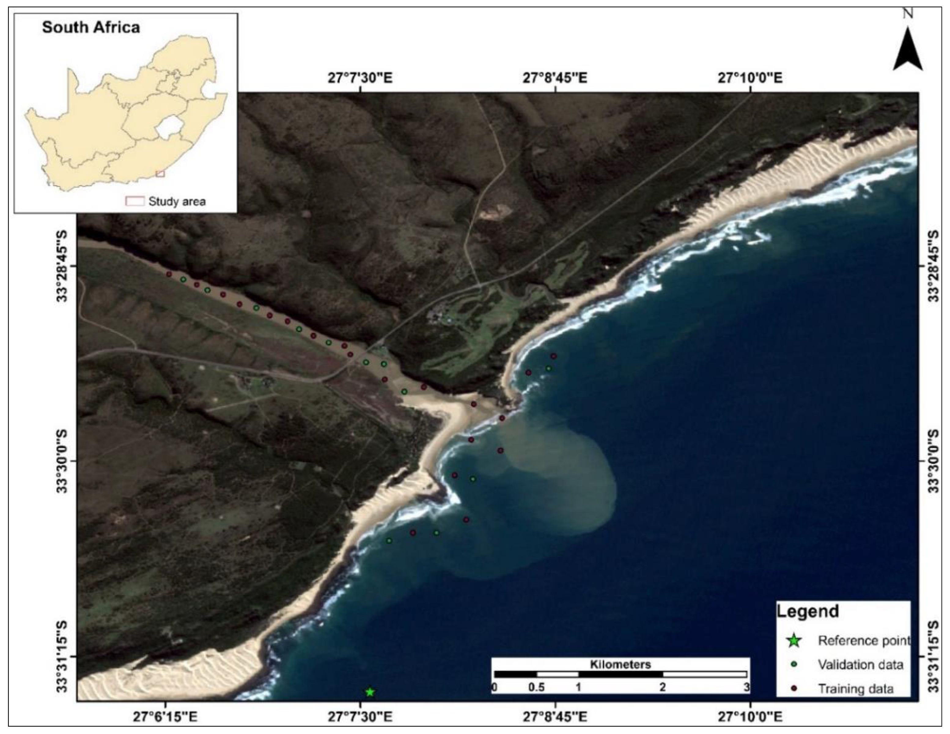
Figure 1. The location of the Great Fish Estuary with respect to South Africa.
Hydrology 11 00164 g001
Figure 2. Schematic flowchart diagram explaining the deployed methodology.
Hydrology 11 00164 g002
Figure 3. Radiance properties of estuarine waters from (a) blue, (b) green, (c) red, (d) red edge 1, (e) red edge 2, (f) red edge 3, (g) NIR, (h) red edge 4, (i) SWIR 1, and (j) SWIR 2 spectral bands.
Hydrology 11 00164 g003
Figure 4. Mean spectral radiance profile of estuarine waters obtained from selected bands.
Hydrology 11 00164 g004
Figure 5. Linear regression results for turbidity against uncalibrated (a) blue, (b) green, (c) red, (d) red edge 1, (e) red edge 2, (f) red edge 3, (g) NIR, (h) red edge 4, (i) SWIR 1, and (j) SWIR 2 spectral bands.
Hydrology 11 00164 g005
Figure 6. Turbidity map produced using IDW (a) and Boolean image generated from the IDW map, using a 50.0 NTU turbidity threshold (b).
Hydrology 11 00164 g006
Figure 7. Linear regression results for turbidity against (a) blue, (b) green, (c) red, (d) red edge 1, (e) red edge 2, (f) red edge 3, (g) NIR, (h) red edge 4, (i) SWIR 1, and (j) SWIR 2 spectral bands calibrated with the sigmoid activation function and SGD.
Hydrology 11 00164 g007
Figure 8. Linear regression results for turbidity against (a) blue, (b) green, (c) red, (d) red edge 1, (e) red edge 2, (f) red edge 3, (g) NIR, (h) red edge 4, (i) SWIR 1, and (j) SWIR 2 spectral bands calibrated with momentum gradient descent.
Hydrology 11 00164 g008
Figure 9. Spatial configuration of turbidity concentration modeled using (a) linear regression on the red band, (b) linear regression on the red band calibrated with the sigmoid function and SGD, (c) linear regression on the green band calibrated with the sigmoid function and MGD, and (d) linear regression on the red band calibrated with the sigmoid function and MGD.
Hydrology 11 00164 g009
Figure 10. R-squared values for performance evaluation of (a) linear regression on the red band, (b) linear regression on the red band calibrated with the sigmoid function and SGD, (c) linear regression on the green band calibrated with the sigmoid function and MGD, and (d) linear regression on the red band calibrated with the sigmoid function and MGD.
Hydrology 11 00164 g010
Table 1. Characteristics of Sentinel-2 spectral bands selected for this study.
Spectral BandWavelength Center (nm)Spatial Resolution (m)
Blue49010
Green56010
Red66510
Red edge 170520
Red edge 274020
Red edge 378320
Near-infrared84210
Red edge 486520
Shortwave infrared 1161020
Shortwave infrared 2219020
Table 2. Learning parameters for MLP-based sigmoid calibration function.
MLP with Sigmoid Activation Function and SGD for Predicting Turbidity from Sentinel-2 Spectral Data
BlueGreenRedNIR
Input specificationsIndependent variablesRadiance values of all bandsRadiance values of all bandsRadiance values of all bandsRadiance values of all bands
Dependent variableRadiance values of blue wavelengthRadiance values of green wavelengthRadiance values of red wavelengthRadiance values of NIR wavelength
Max. training sample used300300300300
Max. testing sample used300300300300
Network topologyNo. of input layer nodes4444
No. of output layer nodes1111
No. of hidden layers2222
Layer 1 nodes5555
Training parametersTraining typeAutomaticAutomaticAutomaticAutomatic
Learning rate typeDynamicDynamicDynamicDynamic
Learning rate start0.010.010.010.01
Learning rate end0.0010.0010.0010.001
Momentum factor0.90.90.90.9
Sigmoid constant1.01.01.01.0
Stopping criteriaIteration10,00010,00010,00010,000
Actual training pixels490497474483
Actual testing pixels491497475483
Learning rate0.0010.0010.0010.001
RMS0.010.010.010.01
Training RMS0.03220.0340.0350.019
Testing RMS0.03440.0370.0330.02
R Sqr.0.9420.9870.9920.979
Table 3. Descriptive statistics of radiance values sampled from selected Sentinel-2 bands.
NDFMinMaxμσSE MeanCoeff. Varp-Value
Blue3002990.2120.2640.2250.0060.0010.03<0.001
Green3002990.2020.2830.2270.0090.0010.04
Red3002990.1690.3230.2280.0160.0010.07
Red edge3002990.0790.2210.1440.020.0010.14
Red edge3002990.1340.3140.1860.0260.0020.14
Red edge3002990.1320.3150.1860.0280.0020.15
NIR3002990.1320.3150.1860.0280.0020.15
Narrow NIR3002990.0950.3050.1380.0320.0020.24
SWIR-13002990.0130.2440.0340.0320.0020.94
SWIR-23002990.0160.090.0210.0080.0010.41
Table 4. Detailed description of the surveyed turbidity.
Statistical ResultsTurbidity
Count40
μ43.31
σ32.34
SE Mean8.84
t-test5.12
p-Value (2-sided)<0.001
UC (2-sided, 95%)63.67
LC (2-sided, 95%)26.89
Table 5. REM results for model performance evaluation.
REM Results
Model M e a n   T m e a s u r e d M e a n   T p r e d i c t e d REM
LR on uncalibrated red band60.4285.21−41.03
MLP on red band calibrated with sigmoid and SGD60.4288.48−46.44
MLP on green band calibrated with sigmoid and MGD60.4272.69−20.31
MLP on red band calibrated with sigmoid and MGD60.4266.06−9.34
Disclaimer/Publisher’s Note: The statements, opinions and data contained in all publications are solely those of the individual author(s) and contributor(s) and not of MDPI and/or the editor(s). MDPI and/or the editor(s) disclaim responsibility for any injury to people or property resulting from any ideas, methods, instructions or products referred to in the content.