Investigating Uncertainty of Future Predictions of Temperature and Precipitation in The Kerman Plain under Climate Change Impacts

Abstract

Climate change affects hydroclimatic variables, and assessing the uncertainty in future predictions is crucial. This study aims to explore variations in temperature and precipitation in the Kerman Plain under climate change impacts between 2023 and 2054. For this purpose, two climate models, MRI-ESM-2 and BCC-CSM2-MR, were used to simulate precipitation and temperature under two different scenarios. The Mann–Kendall test was employed to analyze the annual time series in the future period. The results indicated an increase in the average temperature of about 1.5 degrees Celsius based on both scenarios in the coming years. Furthermore, an average annual increase of 6.37 mm of precipitation was predicted under the SSP585 scenario. Meanwhile, under the SSP585 scenario, an increase was estimated using the MRI-ESM-2 model, and a decrease was predicted with the BCC-CSM2-MR model. The Mann–Kendall test revealed a downward trend in the BCC-CSM2-MR model under both scenarios and an upward trend in the MRI-ESM-2 model under both scenarios. The bootstrap method and the R-factor index were exploited in this study with a 95% confidence interval to estimate the uncertainty of the predicted data. The results demonstrated that the predicted precipitation is more uncertain than the temperature. Finally, it is postulated that the obtained results provide necessary information for water resource management under a changing climate in the study area.

1. Introduction

Climate change refers to long-term alterations in the atmospheric and climatic conditions at local and global scales [1]. These changes can bring about various destructive impacts on water resources. Furthermore, climate change can have different influences on meteorological components, such as precipitation and temperature [2]. Studies have shown that precipitation patterns have undergone changes due to climate change, leading to floods in some areas [3]. The Intergovernmental Panel on Climate Change (IPCC) reports that climate change has more noticeable effects on arid and semi-arid regions of the world [4]. Since Iran has a dry climate, it can have significant impacts on the amount and pattern of precipitation, streamflow, and other hydroclimatic variables [5].

One of the reliable tools for generating climate scenarios is the General Circulation Model (GCM), which predicts future Earth changes [6]. The GCM models describe the Earth’s climate system by dividing it into two layers above and below the sea level, while each layer is divided into smaller networks called cells or networks. Generally, GCMs have a coarse computational grid, which cannot accurately model climate features at sub-grid scales, such as topography or clouds in a local target area. Thus, they are not ready to be used when it comes to providing precise information about temperature and precipitation for hydrological modeling. To overcome this issue, GCM outputs need to be downscaled from a coarse resolution to a finer or even station-scale resolution. One of the techniques utilized to downscale the GCM outputs is exponential micro-scale.

Predictions based on these models rely on different scenarios, each providing information about the socio-economic situation and the amount of greenhouse gas production in the earth’s atmosphere, known as emission scenarios [7]. In this regard, the IPCC presented its latest report (AR6) in 2020. It combined economic–social scenarios and considered the amount of solar energy forcing, called Shared Socio-economic Pathway (SSP) scenarios. The SSP scenarios are mainly classified into five categories, from the most optimistic to the most pessimistic states, providing important insights into the possible effects of climate change in the future [8].

Climate change scenarios do not predict results with 100% reliability. Indeed, there will be uncertainties associated with them due to the assumptions made in each scenario [9]. Since various factors influence predictions for the future, it is not possible to accurately extract and analyze the amount of uncertainty in the obtained results. However, the confidence interval of the achieved results can be extracted and analyzed using some methods, like the bootstrap method [10].

Several studies have been conducted to investigate the impact of climate change on precipitation and temperature. These studies explored trends of precipitation time series using both parametric and non-parametric methods. Additionally, they have examined the uncertainty of climatic parameters. For instance, Gocić and Trajković [11] evaluated annual and seasonal trends in meteorological changes across twelve meteorological stations in Serbia from 1980 to 2010. In their analysis, they employed the M–K test and Sen’s slope to determine trends in meteorological data. Their findings indicated an upward trend in both the minimum and maximum seasonal series of the annual weather, whereas no significant trend was observed in the seasonal precipitation series. They concluded that the M–K test is a reliable method for detecting meteorological trends. Additionally, Fatehifar et al. [12] investigated the effects of climate change by using hydrological indicators in the Azarshahr Chai basin of Iran. They used the CanESM2 model to predict future climate change (2030–2059) under two scenarios (RCP2.6 and RCP8.5). Their results showed an increase in high discharge under both scenarios compared to the base period. However, the average annual discharge was lower than the discharge. Moreover, Singh et al. [13] examined climate change impacts on the Sutlej River Basin in the northwestern Himalayas using two HadCM3 and CGCM3 climate models under scenarios A2, A1B and B2. Their study revealed an overall increase in the average annual temperature and precipitation for future periods. Furthermore, Zahabiyoun et al. [5] evaluated the impact of climate change on the hydrology of one of the main branches of the Karkhe River for the period of 2069–2040. They used the HadCM3-AR4 global climate model data under the A2 scenario. Then, they inserted downscaled climate data into the SWAT model to study future runoff changes. Their results showed that the temperature increased in most months, and the amount of rainfall showed a change in the range of ±30%. Also, Atta-ur-Rahman and Dawood [14] conducted a statistical analysis of temperature trends in the eastern Hindu Kush region of northern Pakistan. They used the M–K test and found an increasing trend in temperature at one station, while another station showed a decreasing trend in the minimum temperature. Their study attributed changes in temperature trends to climate change in the region. In addition, Alamgir et al. [15] determined changes in seasonal droughts in Bangladesh using standardized indexes. They employed 19 GCM models from the fifth IPCC Report and calculated the uncertainty using the bootstrap method at a 95% confidence level. Their findings indicated that the region experiences moderate droughts with the most severe return period. Moreover, Alam et al. [16] predicted the flow of the Brahmaputra River using eight RCP scenarios. They utilized the bootstrap method at a 95% confidence level and reported that the uncertainty in temperature is expected to double in the upcoming years. Furthermore, the average rainfall indicated an increasing trend, and the uncertainty increased significantly from 2020 to 2080. In another study, Goodarzi et al. [17] investigated the impacts of climate change on precipitation in the Gilan province, Iran. They analyzed the historical data between 1980 and 2010 and predicted changes in the region for the coming decades from 2020 to 2100. The M–K test was applied to evaluate the climate issues, and the results showed that the region in question will experience an increase in some areas and a decrease in others. Additionally, their study revealed that the temperature will rise in the coming years. Also, Zeybekoğlu [18] studied the effects of climate change on the Hirfanlı Basin using the M–K test. For this purpose, they evaluated the annual station series between 1965 and 2017 and highlighted that temperatures in the basin have been increasing since the 1990s, which could lead to an increase in the water and meteorological parameters. Consequently, their study predicted that there will be more droughts in the basin in the future. Moreover, Goodarzi et al. [19] studied the impacts of two scenarios from the fifth IPCC report (Rcp8.5 and Rcp2.6) with the output of the HADGEM2 model in the city of Borujard, Iran. Their output showed that the temperature will change by approximately 2.25 °C, and the precipitation will change between 20% and 40% in the next period. Finally, Niazkar et al. [20] utilized a machine learning algorithm to predict the daily weather conditions of Dogonbadan city for the next 30 years (2030–2060) based on two different scenarios (SSP1 and SSP5). They also employed the M–K test to analyze temperature trends and found that the estimated future temperatures are likely to exhibit a growing trend compared with the observed data.

According to the literature, the utilization of the M–K test is common in climate change impact assessment studies. Moreover, the uncertainty evaluation of hydroclimatic variables under a changing climate is essential. Despite previous efforts to quantify the effects of climate change, there is still a need for further investigations, particularly in arid and semi-arid areas, using the scenarios of the sixth IPCC report.

The objective of this study is to analyze the impact of climate change on the temperature and precipitation patterns of the Kerman Plain over the next few decades (2025–2054). It is one of the most significant deserts in Iran. The current study employs the outcomes of selected models from the sixth IPCC report to investigate climate change impacts using the M–K test. Since climate change scenarios are associated with significant uncertainties, the bootstrap method is utilized to assess the accuracy of the predictions. The uncertainty of the predictions is calculated at the 95% confidence level.

2. Materials and Methods

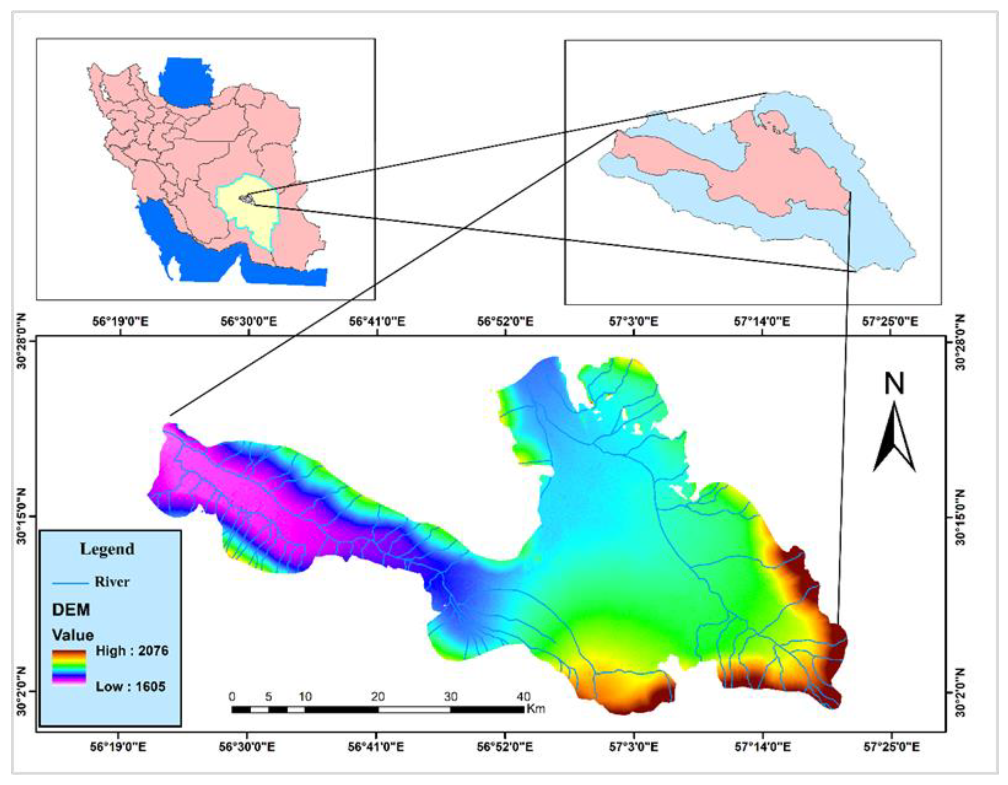
2.1. Study Area

The Kerman Plain is one of twelve areas in the southern region of the Daranjir watershed, Iran. It covers 2030 square kilometers and is between longitudes 56°–19′ and 57°–25′ East and latitudes 30°–2′ and 30°–28′ North. Furthermore, the highest elevation of the area reaches 2076 m, while the lowest point is at the basin outlet, 1605 m. Also, the average annual rainfall of the plain is 132.73 mm, and the average annual temperature is 15.8 °C. The location of the Kerman Plain is illustrated in Figure 1.

2.2. Global Climate Model

To investigate the impacts of climate change on a selected meteorological station, the outputs of two GCM models from the sixth IPCC report were used. The details of the GCM models are presented in

Table 1. Characteristics of the GCM models used in this study.

Source ID	Source Type	Variant Label	Institution Code	Developing Country	Publication Year	Nominal Resolution	Resolution Accuracy (Grade)
BCC-CSM2-MR	AOGCM	r1i1p1	BCC	China	2017	100 km	1.12° × 1.12°
MRI-ESM-2	AOGCM	r1i1p1	CCCma	Japan	2019	100 km	1.12° × 1.12°

. The reason for adopting these two GCM models is their proper performance in the desert region of Kerman Plain and their high ability to simulate meteorological data, which was obtained according to the error indicators [21]. In order to validate the selected models, statistical components, such as the Nash–Sutcliffe coefficient (NSE) and the Root Mean Square Error (RMSE), were used. If these parameters show appropriate values, it indicates the correctness of choosing these models for the intended application.

NSE and RMSE are obtained using the following Equations [21,22]:

$$\mathrm{NSE}=1-\frac{\sum _{i=1}^n{\left(O_i-P_I\right)}^2}{\sum _{i=1}^n{\left[O_i-\overline{O}\right]}^2}$$

(1)

$$\mathrm{RMSE}=\sqrt{\frac{\sum _{i=1}^n{(P_i-O_i)}^2}{n}}$$

(2)

where:

$O_i$= monthly average of observational data;

$P_i$= monthly average predicted by the model;

i = month of the year;

n = number of months;

$\overline{O}$ = the average observational data.

Moreover, the GCM outputs, which include temperature and precipitation, were extracted for the future period of 2025–2054 under two emission scenarios: (i) SSP254 and (ii) SSP585. They predict optimistic and pessimistic conditions for radiative forcing in the atmosphere, respectively [21].

Downscaling

The computational grids used in GCMs are not accurate enough to model climate features, like topography or clouds, at sub-grid levels. Therefore, they cannot provide reliable information on temperature and precipitation data for hydrological modeling [23]. To overcome this issue, it is necessary to downscale the coarse scale of GCM outputs to a finer resolution, even at the scale of individual weather stations [23]. In essence, downscaling is a technique used to downsize global climate change models to local and regional levels. In this study, the LARS-WG statistical downscaling method was utilized to downscale the atmospheric general circulation models. It is one of the most commonly used stochastic data generator models for developing daily irradiance and near-daily precipitation at a station under current and future climate conditions [24,25]. Using historical data, it can forecast daily periods for the future and examine the daily data of public mode networks to provide more accurate predictions [26].

This study analyzed the monthly temperature and precipitation observations measured at the synoptic station of Kerman from 1985 to 2014. The collected data were adopted from the Iranian Meteorological Organization and used as input for the LARS-WG model, along with a scenario file containing temperature and precipitation changes from previous stages. Using the data, the model generated simulated monthly and annual time series for temperature and precipitation at the station for the period between 2025 and 2054.

2.3. Trend Analysis Method

When analyzing weather and meteorological time series, statistical tests are commonly used to check the presence or absence of trends. Several statistical techniques are available to analyze the trends of time series. They are primarily divided into two categories: (i) parametric and (ii) non-parametric. Among these methods, the latter ones are more widely used than the former ones [27,28].

The Mann–Kendall (M–K) test is a non-parametric method exploited to detect an upward or downward trend in hydrological and environmental data. It basically accounts for the data distribution and is resistant to outliers [29]. It also can be exploited to detect trends in time series data regardless of their distribution by examining the relative rankings of data points over time [30]. Furthermore, it is widely used to evaluate hydroclimatic trends [31] and is recommended by the World Meteorological Organization. In this test, values close to zero do not demonstrate any trend, while alternative hypotheses express a trend in a two-sided or one-sided test in an ascending or descending manner [32].

The calculation process of the M–K test is given in Equation (3) [30]:

$$\mathrm{S}={\sum }_{\mathrm{i}=1}^{\mathrm{n}-1}{\sum }_{\mathrm{j}=\mathrm{i}+1}^{\mathrm{n}}\mathrm{s}\mathrm{i}\mathrm{g}\mathrm{n}({\mathrm{x}}_{\mathrm{i}}-{\mathrm{x}}_{\mathrm{k}})$$

(3)

where:

$x_i$ and $x_k$ = sequential data in the series;

n = the number of data points.

The sign function can be computed by Equation (4) [26]:

$$sign (x_i-x_k)=\left\{\begin{array}{c}+1 \mathrm{if} (x_i-x_k)>0\\ 0 \mathrm{if} (x_i-x_k)=0\\ -1 \mathrm{if} (x_i-x_k)<0\end{array}\right.$$

(4)

If n > 10, the S statistic is normally distributed to obtain the standard normal variance (Z) [33]. In addition, the significance level α is utilized to determine if there is a statistically significant change in the data. Z > 0 and Z < 0 indicate an increasing and a negative trend, respectively. However, if Z is not greater than 1 − 0.5α, which does not correspond to a standard normal, it is not possible to determine a trend based on the available data [34].

2.4. Sequential Mann–Kendall Test

The Sequential Mann–Kendall (S-MK) test is used to display graphical results and identify trends over time [29]. The test statistic t is obtained by summing n_i, which is the number of values smaller than the previous ranks for each rank. The average value of t and its expected value are calculated using Equations (5) and (6), respectively [35,36]:

$$t={\sum }_{i=1}^n{n}_i$$

(5)

$$E(t)=\frac{\mathrm{n}(\mathrm{n}-1)}{4}$$

(6)

The variance of t (Var(t)) is computed using Equation (7):

$$\mathit{Var}(t)=\frac{n(n-1)(2n+5)}{72}$$

(7)

Based on Equation (8), the test statistic u(t) can be obtained:

$$\mathit{u}(t)=\frac{(t-E(t\left)\right)}{\sqrt{Var\left(t\right)}}$$

(8)

The inverse test statistic u′(t) is calculated in a similar manner as u(t). At the point where u(t) intersects with u’(t), it indicates the starting point of the process [36].

2.5. Uncertainty Analysis

Bootstrap is a technique used to estimate the uncertainty in statistical models by resampling the data. It involves creating multiple bootstrap samples and calculating desired statistics in each sample. In the context of climate modeling, the bootstrap can be employed to assess the uncertainty of the outputs of statistical models simulating hydroclimatic variables, such as temperature and precipitation. It is particularly useful in providing a more accurate representation of the range of possible values for temperature and precipitation [37,38].

To calculate uncertainty, 10,000 values are randomly selected from the available data. At each selection stage, the desired statistics are computed, and a normal distribution is fitted. Finally, considering a 95% confidence interval, the upper and lower limits of the values are determined [39]. To compute the uncertainty of the data, the R-factor criterion can be calculated using Equation (9) [39]:

$$\mathrm{R}-\mathrm{factor}=\frac{CI}{{\sigma }_x}$$

(9)

where:

${\sigma }_x$ = the standard deviation of the variable x;

CI = the average distance between the upper and lower limits and can be computed by Equation (10):

$$CI=\frac{1}{k}{\sum }_{i=1}^k{(x}_u-x_l)$$

(10)

where:

$x_u$ = 97.5% percentile;

$x_l$ = 2.5% percentile;

k = the number of predicted data points.

R-factor can be adjusted from 1 to infinity, while lower values of R-factor suggest fewer outliers and more reliable results.

3. Results

3.1. Annual Changes in Precipitation

The LARS-WG model was used to generate climatic parameters for temperature and precipitation between 2025 and 2054. These hydroclimatic variables were then simulated under two different GCM models (MRI-ESM-2 and BCC-CSM2-MR) and two scenarios (SSP245 and SSP585).

Table 2. Annual changes of simulated future precipitation under the climate models and scenarios compared to observed precipitations.

Station Name	Annual Average Precipitation in the Observation Period (1985 to 2014) (mm)	GCM Model	Climate Scenario	Annual Average Precipitation in the Future (2025 to 2054) (mm)	Future Precipitation Changes Compared to the Base Period (mm)	The Percentage of Future Precipitation Changes Compared to the Base Period
Kerman plain	130.62	BCC-CSM2-MR	SSP245	146.04	15.42	11.8
			SSP585	147.54	16.92	12.95
		MRI-ESM-2	SSP245	127.86	−2.76	−2.11
			SSP585	131.86	1.24	0.94

presents the results of the predicted annual precipitation changes compared to the base period values. As shown, the obtained results indicate that, except for the SSP245 scenario in the MRI-ESM-2 model, all other models and scenarios predict an increase in precipitation from 2025 to 2054. It is worth noting that both models forecast a higher increase under the SSP585 scenario compared to that of the SSP245 scenario. Furthermore, the results of the simulations show that, under the MRI-ESM-2 model and SSP245 scenario, the annual precipitation in the Kerman station has decreased. However, all other models and scenarios predict an increase in precipitation during the same period. On average, over the next 30 years, it is expected that there will be an increase in the coming years.

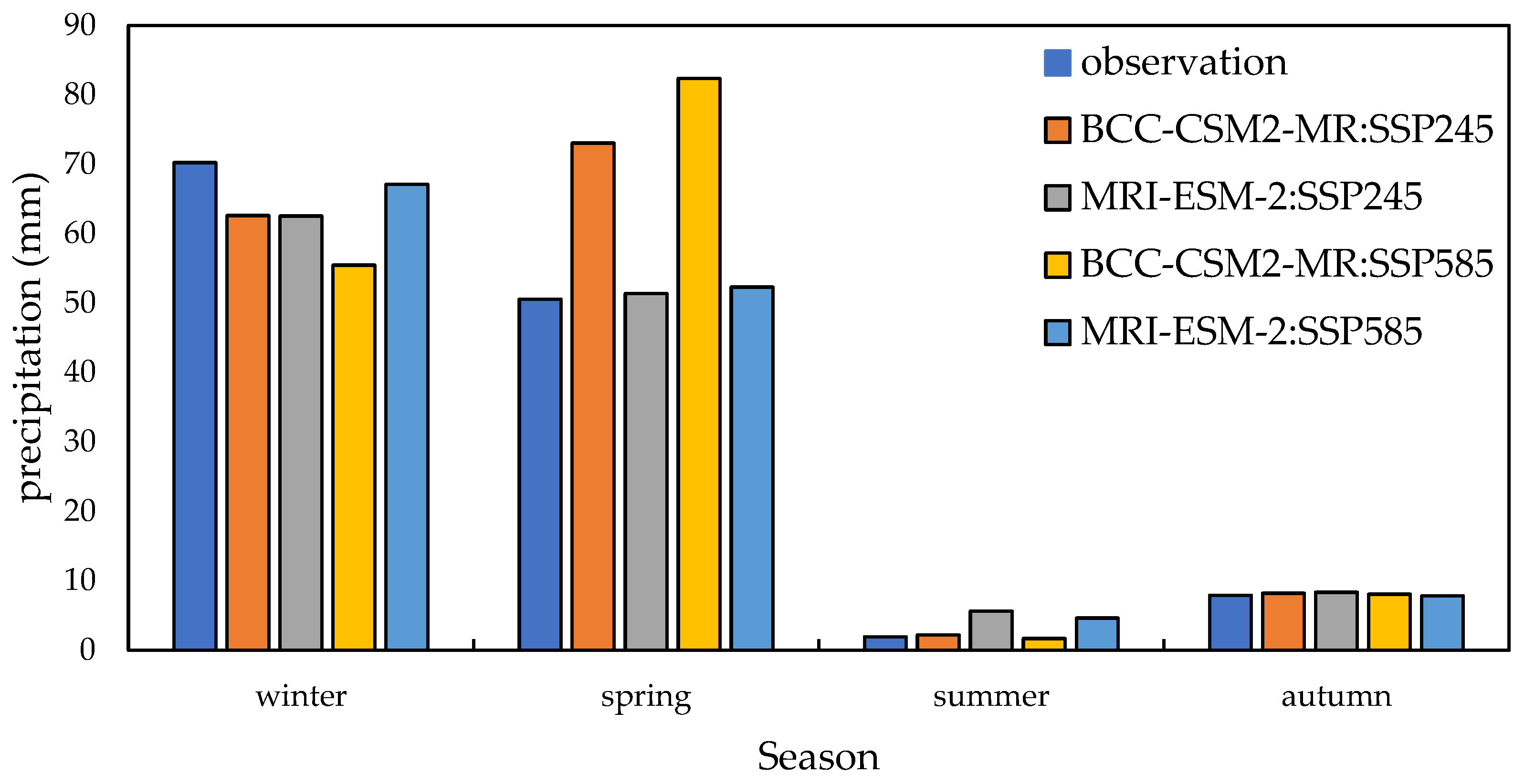
3.2. Seasonal Changes in Precipitation

Figure 2 reveals that the precipitation patterns in the Kerman Plain undergo seasonal changes. Over time, there will be a decrease in winter precipitation and an increase in spring precipitation. The increase in spring precipitation is a significant factor in predicting an annual increase in precipitation in the upcoming years (2025–2054). The BCC-CSM2-MR model under the SSP585 scenario estimates the highest spring precipitations, while the MRI-ESM-2 model under the SSP245 scenario predicts the lowest increase. Nevertheless, the spring precipitations are mainly of the rain type, which increases the likelihood of floods occurring in the area under investigation.

3.3. Annual Changes in Temperature

Table 3. Annual changes in the minimum temperature of the future simulation using climate models and scenarios in the future period (2025–2054) compared with the observation period (1985–2014).

Station Name	Annual Minimum Temperature during the Observation Period (1985 to 2014) (°C)	GCM Model	Climate Scenario	Annual Minimum Temperature in the Future (2025 to 2054) (°C)	Future Temperature Changes Compared to the Base Period (°C)
Kerman plain	7.38	BCC-CSM2-MR	SSP245	8.59	1.21
			SSP585	8.73	1.35
		MRI-ESM-2	SSP245	7.95	0.57
			SSP585	8.46	1.08

and

Table 4. Annual changes in the maximum temperature of the future simulation using climate models and scenarios in the future period (2025–2054) compared with the observation period (1985–2014).

Station Name	Annual Maximum Temperature during the Observation Period (1985 to 2014) (°C)	GCM Model	Climate Scenario	Annual Maximum Temperature in the Future (2025 to 2054) (°C)	Future Temperature Changes Compared to the Base Period (°C)
Kerman plain	25.27	BCC-CSM2-MR	SSP245	26.97	1.7
			SSP585	27.07	1.82
		MRI-ESM-2	SSP245	25.86	0.62
			SSP585	26.48	1.21

provide a detailed summary of the estimated changes in the minimum and maximum annual temperature in the future period compared with the observation period. According to the LARS-WG predictions, the minimum and maximum annual temperature (T_min and T_max) in the Kerman Plain will increase in the coming years, regardless of the selected climate models and scenarios. The BCC-CSM2-MR model estimates the highest increase of maximum temperature by 1.82 °C under the SSP585 scenario, while the MRI-ESM-2 model projects the lowest increase of minimum temperature by 0.57 °C under the SSP245 scenario.

According to the results shown in Table 3 and Table 4, the annual maximum and minimum temperatures are expected to increase in the future period under all selected climate models and scenarios. In addition, both GCM models forecast a higher annual temperature increase under the SSP585 scenario compared with that of the SSP245 scenario. Therefore, it can be concluded that the SSP585 scenario is the most pessimistic scenario for temperature, as it predicts a higher temperature increase for the studied area. Moreover, the rise in the temperature and the projected increase in precipitation in the Kerman Plain have been observed in previous studies, which indicated that the emission scenarios with the highest increase in greenhouse gases (A2 and RCP8.5 scenarios), such as the SSP585 scenario, predicted an increase in both precipitation and temperature [40].

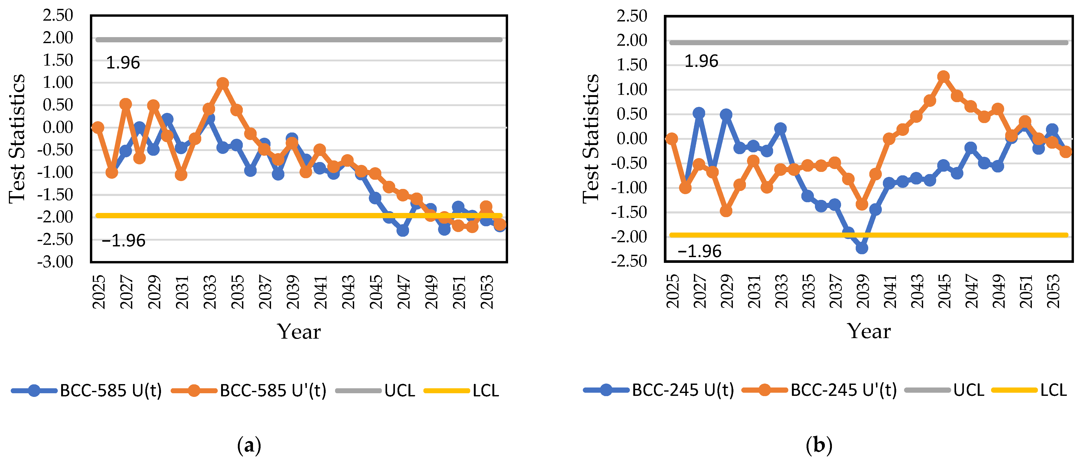
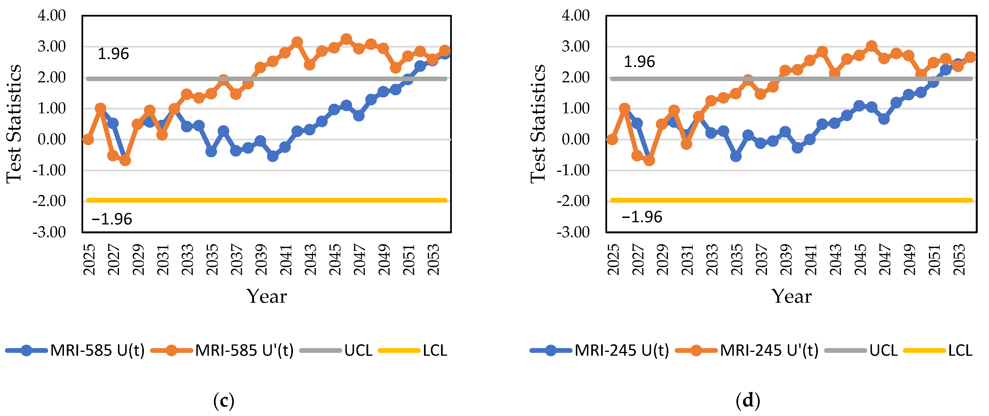
3.4. Trends in Annual Precipitation Changes

The statistics of the S-MK test were calculated for each climate model, and Figure 3 displays u(t_i) and u’(t_i) for each model. The confidence level for this test is 5%, and all analyses were conducted based on the u(t_i) and u’(t_i) values. A time series is considered significant when u > 1.96 or u < −1.96. Based on the analysis of the results presented in Figure 3, it can be concluded that there is a declining trend in the BCC245 model between 2034 and 2039. Furthermore, there is no discernible trend for the rest of the predicted period, whereas there will be changes in the final years of the process. Moreover, the BCC585 model underwent various mutations, and the process began in 2043. The MRI 585 and MRI245 models show that the u(t_i) and u’(t_i) graphs intersect each other in the positive area in 2032 and indicate the start of an upward trend in the positive direction, which continues till the end of the studied period. This implies that there will be an increase in precipitation from 2032 to 2054.

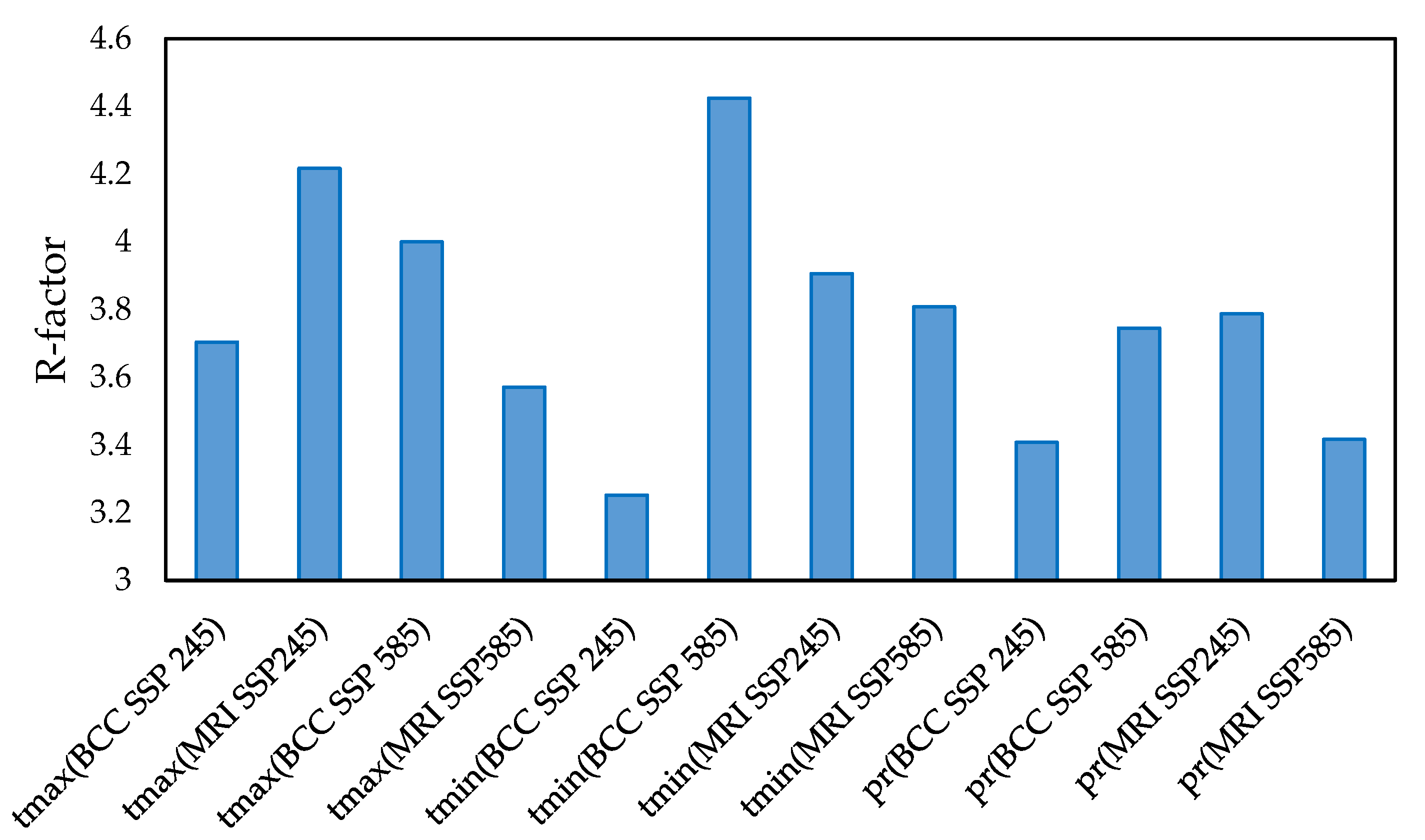
3.5. Assessment of the Uncertainty of Temperature and Precipitation Predictions

In this study, two models were used to predict the maximum and minimum temperatures, as well as precipitation levels, for the years 2025 to 2054. Two climate change scenarios were also taken into consideration. To determine the uncertainty of the obtained values, the bootstrap method was utilized, and the R 4.2.1 software was used for analysis. The results were then used to determine the 95% confidence interval, the upper limit of 97.5%, the lower limit of 2.5%, and the R-factor index for each of the maximum temperature, minimum temperature, and precipitation data. The uncertainty results are presented in

Table 5. Uncertainty results of precipitation and temperature under climate change scenarios.

Climatic Parameter	Mean	Median	Standard Deviation	2.5%	97.5%	R-Factor
Tmax (BCC-SSP245)	28.78	28.8	0.162	28.5	29.1	3.70
Tmin (BCC-SSP245)	9.5	9.5	0.123	9.3	9.7	3.25
Tmin (BCC-SSP585)	9.53	9.5	0.113	9.3	9.8	4.42
Tmax (BCC-SSP585)	28.67	28.67	0.175	28.3	29	4
Tmin (MRI-SSP245)	8.47	8.47	0.128	8.2	8.7	3.90
Tmax (MRI-SSP245)	26.87	26.78	0.166	26.4	27.1	4.21
Tmin (MRI-SSP585)	8.94	8.94	0.1313	8.7	9.2	3.80
Tmax (MRI-SSP585)	27.32	27.32	0.168	27	27.6	3.57
Pr (BCC-SSP245)	132.32	126.8	18.78	109	173	3.41
Pr (BCC-SSP585)	144.48	145.2	10.76	126.7	167	3.74
Pr (MRI-SSP245)	123.989	118.65	11.09	105.9	147.9	3.78
Pr (MRI-SSP585)	128.91	123.95	11.97	110.1	151	3.42

. To be more specific, it shows the average, median, standard deviation, upper and lower limits of maximum and minimum temperatures, and precipitation in climate models and scenarios. According to Table 5, the standard deviation values of the predicted temperatures range between 0.1 and 0.2, indicating that predicted temperatures are closer to the average temperature and, consequently, they are less scattered. Additionally, the minimum temperature predicted by the BCC-SSP585 scenario has the lowest standard deviation value of 0.113 compared to other predicted temperatures. Also, the maximum temperature predicted by the same scenario has the highest standard deviation value of 0.175.

Based on Table 5, the predicted precipitations have a higher standard deviation. This implies that the data are more dispersed than the corresponding average precipitation. However, since the precipitation values are not more than twice the average, they cannot be considered outliers. Furthermore, the BCC-SSP245 scenario has the highest standard deviation in precipitation with a value of 18.78, whereas the BCC-SSP585 scenario has the lowest standard deviation with a value of 10.76.

The R-factor index was used to compare the uncertainty of the available data. The temperature and precipitation results for each scenario are presented in Table 5 and Figure 4. As shown, all R-factor values range between 3 and 4.5. The lower the R-factor value, the more reliable the data and the fewer outliers present. Among the temperature data, the lowest R-factor value corresponds to the predicted minimum temperature under the BCC SSP245 scenario, with a value of 3.25. On the other hand, the highest R-factor value corresponds to the minimum temperature under the BCC SSP585 scenario, with a value of 4.42. Similarly, in the case of precipitation, the lowest R-factor value is related to the precipitation obtained under the BCC SSP245 scenario, with a value of 3.41. Moreover, the highest R-factor value is related to the predicted precipitation under the MRI SSP245 scenario, with a value of 3.78. Overall, the R-factor values for all climate change scenarios are very close to each other, indicating the consistency and reliability of the data.

Figure 5 displays the confidence intervals, which are placed beside the average of predicted temperatures and precipitations. Obviously, the confidence interval of the minimum temperature is lower than that of the maximum temperature. Additionally, the predicted temperatures under the BCC scenarios tend to be higher than those achieved under the MRI scenarios. According to the results, the 95% confidence interval of precipitations is higher than that of the temperatures, which is in line with the results of the standard deviation and R-factor.

4. Discussion

In this study, the trend of temperature and precipitation changes in Iran’s Kerman Plain during the coming years (2025–2054) was investigated. Then, the uncertainty of hydroclimatic variables was calculated and measured using the bootstrap method and the R-factor index. The primary goal was to predict the temperature and precipitation of this region in the coming years, which was conducted with the LARS-WG model using observational data analysis in the past years (1985–2014). In order to predict climate data, two CMIP6 models (BCC-CSM2-MR and MRI-ESM-2) were used under two scenarios (SSP245 and SSP585) due to their proper performances in the studied area. The modeling results provided us with valuable insights about the climate and conditions of the Kerman Plain in the coming years. Similar studies in the literature have investigated the effect of climate change on precipitation and temperature. Notably, they reviewed theoretical issues that are aligned with the objectives of this study [5,17]. Zahabiyoun et al. [5] emphasized the importance of investigating the impact of climate change on river hydrology, while Goodarzi et al. [17] specifically focused on precipitation and temperature. These studies, together with our research, contribute to a wider understanding of the importance of climate change on the water status of different regions and provide valuable insights into the climatic conditions of the coming years, especially in the arid and semi-arid regions of Iran. According to the results, precipitation will increase by 11.8% in the future under the SSP245 scenario and 12.95% and 0.94% under the SSP585 scenarios of both models compared with the observations of the base period.

5. Conclusions

In conclusion, based on the investigation of seasonal precipitation patterns, it is predicted that there will be a gradual decrease in winter precipitation and an increase in spring precipitation in the coming years, respectively. Furthermore, the minimum temperature is expected to increase by 0.57 to 1.21 degrees under SSP 245 and 1.08 to 1.35 degrees under SSP585 compared with those of the base period, and the maximum temperature is expected to increase by 0.62 to 1.7 degrees under SSP 245 and 1.21 to 1.82 degrees under SSP585 compared with those of the base period, respectively. Due to the increase in temperature and unusual precipitation patterns, it is likely that the region under consideration will experience floods in spring. The results of the Man–Kendall test revealed that the BCC-CSM2-MR climate model predicts a generally downward trend of precipitation changes under both SSP245 and SSP585 scenarios, whereas the MRI-ESM-2 climate model estimates an overall upward trend of precipitation changes under both scenarios. Moreover, the BCC-CSM2-MR model forecasts an increase in the annual precipitation, whereas a decreasing trend was identified. It implies that future conditions will worsen despite the predicted increase in precipitation. The predicted increase in the precipitation is significant despite the rise in temperature and the shift in the precipitation patterns. Additionally, the MRI-ESM-2 model shows an upward trend in both climate scenarios, even though it predicts a lower increase in precipitation compared to that of the other model. This trend could be attributed to the rise in cloud condensation nuclei caused by particle pollution resulting from industrial development and population growth in the Kerman province. The predicted data under different scenarios have some level of uncertainty; the bootstrap method and the R-factor index were utilized to investigate the 95% confidence interval and the upper and lower limits of 97.5% and 2.5% of the predicted values of temperature and precipitation. The results indicate that the 95% confidence interval in the precipitation data was wider than that of the predicted temperature data, indicating that the latter has less uncertainty. Also, the standard deviation of the temperature data was lower than that of the precipitation, indicating a lower dispersion of temperature values compared with the corresponding average. Overall, the results suggested that while precipitation has been increasing, the probability of flooding in the region has also increased, particularly in shorter periods of time. Therefore, it is important to take necessary measures and preparations not only to address this issue but also to better manage water consumption through improved water planning.

Despite the progress made in this study, some limitations should also be mentioned. The LARS-WG statistical model is a numerical model associated with a percentage of errors and may not fully represent the complexities inherent in simulating future data. In addition, the climate models used in this study and generally all climate models that are currently available, may not be able to provide an accurate prediction of the future situation. Hence, further investigations are necessary to validate the method, considering a wider number of climate models and scenarios.

References

1. Goyal, R.; Gaur, M.K. The Implications of Climate Change on Water Resources of Rajasthan, in Hydro-Meteorological Extremes and Disasters; Springer: Berlin/Heidelberg, Germany, 2022; pp. 265–278. [Google Scholar] [CrossRef]
2. Stocker, T. Climate Change 2013: The Physical Science Basis: Working Group I Contribution to the Fifth Assessment Report of the Intergovernmental Panel on Climate Change; Cambridge University Press: Cambridge, UK, 2014. [Google Scholar]
3. Wang, B.; Kim, H.-J.; Kikuchi, K.; Kitoh, A. Diagnostic metrics for evaluation of annual and diurnal cycles. Clim. Dyn. 2010, 37, 941–955. [Google Scholar] [CrossRef]
4. Pachauri, R.K.; Allen, M.R.; Barros, V.R.; Broome, J.; Cramer, W.; Christ, R.; Church, J.A.; Clarke, L.; Dahe, Q.; Dasgupta, P.; et al. Climate Change 2014: Synthesis Report. Contribution of Working Groups I, II and III to the Fifth Assessment Report of the Intergovernmental Panel on Climate Change; Cambridge University Press: Cambridge UK; New York, NY, USA; IPCC: Geneva, Switzerland, 2014. [Google Scholar]
5. Zahabiyoun, B.; Goodarzi, M.R.; Bavani, A.R.M.; Azamathulla, H.M. Assessment of Climate Change Impact on the Gharesou River Basin Using SWAT Hydrological Model. CLEAN Soil Air Water 2013, 41, 601–609. [Google Scholar] [CrossRef]
6. Mitchell, T.D. Pattern Scaling: An Examination of the Accuracy of the Technique for Describing Future Climates. Clim. Chang. 2003, 60, 217–242. [Google Scholar] [CrossRef]
7. Carter, T.; Hulme, M.; Lal, M. General Guidelines on the Use of Scenario Data for Climate Impact and Adaptation Assessment; Finnish Environmental Institute: Helsinki, Finland, 2007. [Google Scholar]
8. Gupta, V.; Singh, V.; Jain, M.K. Assessment of precipitation extremes in India during the 21st century under SSP1-1.9 mitigation scenarios of CMIP6 GCMs. J. Hydrol. 2020, 590, 125422. [Google Scholar] [CrossRef]
9. Katz, R. Techniques for estimating uncertainty in climate change scenarios and impact studies. Clim. Res. 2002, 20, 167–185. [Google Scholar] [CrossRef]
10. Thai, H.; Mentré, F.; Holford, N.H.; Veyrat-Follet, C.; Comets, E. A comparison of bootstrap approaches for estimating uncertainty of parameters in linear mixed-effects models. Pharm. Stat. 2013, 12, 129–140. [Google Scholar] [CrossRef]
11. Gocic, M.; Trajkovic, S. Analysis of changes in meteorological variables using Mann-Kendall and Sen’s slope estimator statistical tests in Serbia. Glob. Planet. Chang. 2013, 100, 172–182. [Google Scholar] [CrossRef]
12. Fatehifar, A.; Goodarzi, M.R.; Hedesh, S.S.M.; Dastjerdi, P.S. Assessing watershed hydrological response to climate change based on signature indices. J. Water Clim. Chang. 2021, 12, 2579–2593. [Google Scholar] [CrossRef]
13. Singh, D.; Gupta, R.D.; Jain, S.K. Assessment of impact of climate change on water resources in a hilly river basin. Arab. J. Geosci. 2015, 8, 10625–10646. [Google Scholar] [CrossRef]
14. Rahman, A.U.; Dawood, M. Spatio-statistical analysis of temperature fluctuation using Mann–Kendall and Sen’s slope approach. Clim. Dyn. 2017, 48, 783–797. [Google Scholar] [CrossRef]
15. Alamgir, M.; Khan, N.; Shahid, S.; Yaseen, Z.M.; Dewan, A.; Hassan, Q.; Rasheed, B. Evaluating severity–area–frequency (SAF) of seasonal droughts in Bangladesh under climate change scenarios. Stoch. Environ. Res. Risk Assess. 2020, 34, 447–464. [Google Scholar] [CrossRef]
16. Alam, S.; Ali, M.; Rahaman, A.Z.; Islam, Z. Multi-model ensemble projection of mean and extreme streamflow of Brahmaputra River Basin under the impact of climate change. J. Water Clim. Chang. 2021, 12, 2026–2044. [Google Scholar] [CrossRef]
17. Goodarzi, M.R.; Abedi, M.J.; Pour, M.H. Climate change and trend analysis of precipitation and temperature: A case study of Gilan, Iran. In Current Directions in Water Scarcity Research; Elsevier: Amsterdam, The Netherlands, 2022; pp. 561–587. [Google Scholar] [CrossRef]
18. Zeybekoğlu, U. Temperature series analysis of the Hirfanli Dam Basin with the Mann-Kendall and Sequential Mann-Kendall tests. Turk. J. Eng. 2023, 7, 306–313. [Google Scholar] [CrossRef]
19. Goodarzi, M.R.; Mohtar, R.H.; Piryaei, R.; Fatehifar, A.; Niazkar, M. Urban WEF Nexus: An Approach for the Use of Internal Resources under Climate Change. Hydrology 2022, 9, 176. [Google Scholar] [CrossRef]
20. Niazkar, M.; Goodarzi, M.R.; Fatehifar, A.; Abedi, M.J. Machine learning-based downscaling: Application of multi-gene genetic programming for downscaling daily temperature at Dogonbadan, Iran, under CMIP6 scenarios. Theor. Appl. Clim. 2023, 151, 153–168. [Google Scholar] [CrossRef]
21. Zarrin, A.; Dadashi-Rodbari, A.; Salehabadi, N. Projected temperature anomalies and trends in different climate zones in Iran based on CMIP6. Iran Geophys. J. 2021, 15, 35–54. [Google Scholar] [CrossRef]
22. Gupta, H.V.; Kling, H.; Yilmaz, K.K.; Martinez, G.F. Decomposition of the mean squared error and NSE performance criteria: Implications for improving hydrological modelling. J. Hydrol. 2009, 377, 80–91. [Google Scholar] [CrossRef]
23. Wilby, R.; Dawson, C.; Barrow, E. SDSM—A decision support tool for the assessment of regional climate change impacts. Environ. Model. Softw. 2002, 17, 145–157. [Google Scholar] [CrossRef]
24. Adnan, R.M.; Liang, Z.; Trajkovic, S.; Zounemat-Kermani, M.; Li, B.; Kisi, O. Daily streamflow prediction using optimally pruned extreme learning machine. J. Hydrol. 2019, 577, 123981. [Google Scholar] [CrossRef]
25. Rajabi, A.; Sedghi, H.; Eslamian, S.S.; Musavi, H. Comparison of Lars-WG and SDSM downscaling models in Kermanshah (Iran). Ecol. Environ. Conserv. 2010, 16, 1–7. [Google Scholar]
26. Semenov, M.A.; Barrow, E.M.; Lars-Wg, A. A Stochastic Weather Generator for Use in Climate Impact Studies; User Manual: Hertfordshire, UK, 2002. [Google Scholar]
27. Bihrat, Ö.; Bayazit, M. The power of statistical tests for trend detection. Turk. J. Eng. Environ. Sci. 2003, 27, 247–251. [Google Scholar]
28. Takeuchi, K.; Xu, Z.; Ishidiaira, H. Monitoring trend step changes in precipitation in Japanese precipitation. J. Hydrol. 2003, 279, 144–150. [Google Scholar]
29. Hırca, T.; Türkkan, G.E.; Niazkar, M. Applications of innovative polygonal trend analyses to precipitation series of Eastern Black Sea Basin, Turkey. Theor. Appl. Clim. 2021, 147, 651–667. [Google Scholar] [CrossRef]
30. Nashwan, M.S.; Shahid, S. Spatial distribution of unidirectional trends in climate and weather extremes in Nile river basin. Theor. Appl. Clim. 2019, 137, 1181–1199. [Google Scholar] [CrossRef]
31. Ahmed, K.; Shahid, S.; Wang, X.; Nawaz, N.; Khan, N. Spatiotemporal changes in aridity of Pakistan during 1901–2016. Hydrol. Earth Syst. Sci. 2019, 23, 3081–3096. [Google Scholar] [CrossRef]
32. Pohlert, T. Non-Parametric Trend Tests and Change-Point Detection. 2018. Available online: https://cran.r-project.org/web/packages/trend/trend.pdf (accessed on 15 July 2023).
33. Niazkar, M.; Piraei, R.; Türkkan, G.E.; Hırca, T.; Gangi, F.; Afzali, S.H. Drought analysis using innovative trend analysis and machine learning models for Eastern Black Sea Basin. Theor. Appl. Clim. 2023, 1–20. [Google Scholar] [CrossRef]
34. Lee, J.M.; Kwon, E.H.; Woo, N.C. Natural and Human-Induced Drivers of Groundwater Sustainability: A Case Study of the Mangyeong River Basin in Korea. Sustainability 2019, 11, 1486. [Google Scholar] [CrossRef]
35. Gilbert, R.O. Statistical Methods for Environmental Pollution Monitoring; John Wiley & Sons: Hoboken, NJ, USA, 1987. [Google Scholar]
36. Gumus, V.; Yenigun, K. Evaluation of Lower Firat Basin streamflow by trend analysis. In Proceedings of the 7th International Advances in Civil Engineering Conference, Istanbul, Turkey, 10–13 October 2006. [Google Scholar] [CrossRef]
37. Gouvea, L.F.; Ara, A.; Gigante, R.L.; Spatti, R.A.; Louzada, F. Bootstrap resampling as a tool for calculating uncertainty measurement. Braz. Appl. Sci. Rev. 2020, 4, 901–912. [Google Scholar] [CrossRef]
38. Lubke, G.H.; Campbell, I.; McArtor, D.; Miller, P.; Luningham, J.; van den Berg, S.M. Assessing Model Selection Uncertainty Using a Bootstrap Approach: An Update. Struct. Equ. Model. Multidiscip. J. 2016, 24, 230–245. [Google Scholar] [CrossRef]
39. Nakhaei, M.; Ghazban, F.; Nakhaei, P.; Gheibi, M.; Wacławek, S.; Ahmadi, M. Successive-Station Streamflow Prediction and Precipitation Uncertainty Analysis in the Zarrineh River Basin Using a Machine Learning Technique. Water 2023, 15, 999. [Google Scholar] [CrossRef]
40. Mesbahzadeh, T.; Miglietta, M.M.; Mirakbari, M.; Sardoo, F.S.; Abdolhoseini, M. Joint Modeling of Precipitation and Temperature Using Copula Theory for Current and Future Prediction under Climate Change Scenarios in Arid Lands (Case Study, Kerman Province, Iran). Adv. Meteorol. 2019, 2019, 6848049. [Google Scholar] [CrossRef]
Figure 1. Location of the Kerman Plain.
Hydrology 11 00002 g001
Figure 2. Seasonal average of precipitation under two climate models and scenarios for the future period (2025–2054) compared with the values of the observation period (1985–2014).
Hydrology 11 00002 g002
Figure 3. Results of trend analysis of climate models from 2025 to 2054. (a) BCC-CSM2-MR under SSP585 scenario; (b) BCC-CSM2-MR under SSP245 scenario; (c) MRI-ESM-2 under SSP585 scenario; (d) MRI-ESM-2 under SSP245 scenario. (Upper confidence limit (UCL) and lower confidence limit (LCL) are represented by +1.96 and −1.96, respectively).
Hydrology 11 00002 g003aHydrology 11 00002 g003b
Figure 4. R-factor criterion of temperature and precipitation under climate change scenarios.
Hydrology 11 00002 g004
Figure 5. The 95% confidence interval of (a) minimum temperature, (b) maximum temperature, and (c) precipitation values under two models and two scenarios.
Hydrology 11 00002 g005