Abstract
This study configures the Weather Research and Forecasting (WRF) model with the updated urban fraction for optimal rainfall simulation over Kampala, Uganda. The urban parameter values associated with urban fractions are adjusted based on literature reviews. An extreme rainfall event that triggered a flood hazard in Kampala on 25 June 2012 is used for the model simulation. Observed rainfall from two gauging stations and satellite rainfall from Climate Hazards Group InfraRed Precipitation with Station data (CHIRPS) are used for model validation. We compared the simulation using the default urban fraction with the updated urban fraction focusing on extreme rainfall amount and spatial-temporal rainfall distribution. Results indicate that the simulated rainfall is overestimated compared to CHIRPS and underestimated when comparing gridcell values with gauging station records. However, the simulation with updated urban fraction shows relatively better results with a lower absolute relative error score than when using default simulation. Our findings indicated that the WRF model configuration with default urban fraction produces rainfall amount and its spatial distribution outside the city boundary. In contrast, the updated urban fraction has peak rainfall events within the urban catchment boundary, indicating that a proper Numerical Weather Prediction rainfall simulation must consider the urban morphological impact. The satellite-derived urban fraction represents a more realistic urban extent and intensity than the default urban fraction and, thus, produces more realistic rainfall characteristics over the city. The use of explicit urban fractions will be crucial for assessing the effects of spatial differences in the urban morphology within an urban fraction, which is vital for understanding the role of urban green areas on the local climate.
1. Introduction
Numerical weather prediction (NWP) models, such as Weather Research and Forecasting (WRF), are nowadays used for flood hazard modeling and forecasting in urban areas [1,2]. However, simulating the spatial–temporal rainfall characteristics and structures that trigger flood hazards is challenging and complex to predict. The mechanisms affecting rainfall are affected by many factors: the quality of initial and boundary conditions, domain set, and parametrization schemes in model [3]. The urban landscape characteristics, such as urban fraction and urban parameters, are essential factors in the urban parameterization schemes that affect the simulated extreme rainfall triggering floods in the urban areas. Changes in the urban landscape alter the near-surface radiation and energy budgets, momentum, and water vapor in urban areas, which affect the initiation and intensification of convective processes over a city [4]. Moreover, with an urban expansion, a larger thermal contrast between the urban areas and the water body can result in stronger low-level circulation [5]. Consequently, meteorological conditions alter; thus, it determines the formation of convection storms and intensive rainfall over urban areas [6,7,8]. In the numerical weather prediction models, the impact of such urban surface change can be handled through land-surface modeling implemented in parameterization schemes.
The WRF model is widely used to examine and assess the impact of the urban landscape on hydrometeorological processes leading to changes in high-intensity rainfall events. In the WRF model, these processes are addressed using urban parameterization schemes, for instance, the Single-Layer Urban Canopy Model (SLUCM) [9]. A variety of studies have been carried out using the WRF model to improve its skills in assessing the impact of the urban landscape on meteorological fields leading to extreme rainfall events [10,11,12,13,14].
However, the default urban fraction and the corresponding parameter in the WRF model incorrectly represent the true extent and values of the urban surfaces for individual cities. For instance, the default urban fraction in the WRF model, which is provided by Moderate-resolution Imaging Spectroradiometer (MODIS) observational data, cannot fully represent the correct extent and position of the urban area. Urban parameter values are also site-specific and incorrectly represent a city’s extent and position; hence, it needs to be updated, as suggested by [7,15,16,17]. Therefore, the correct representation of the city’s urban fraction is required to optimally simulate the high-intensity rainfall distribution over the urban area. This study uses the detailed and high-resolution urban fraction generated using Landsat image instead of the default MODIS urban fraction. This Landsat image is highly detailed and able to capture detailed urban features, such as wetlands and individual urban fractions at 30 m resolution, which proved to be applicable for hydrological process modeling leading to flooding in Kampala. Here, we updated the default urban fraction in the WRF model primarily to represent the correct position and extent of the city and, secondly, to use a consistent urban fraction for integrated flood hazard modeling and the WRF model.
Several other urban fractions have been developed for different atmospheric modeling purposes. For example, local climate zoning (LCZ) is designed to study the thermal characteristics of urban areas [8,18], and in-homogeneous urban canopy parameters (UCP) are developed for air quality modeling [6]. In this study, the urban fraction derived from the Landsat image of 2016, initially developed for urban land-use planning and flood management [19], is used in the WRF model. Therefore, this study is the first order to study the role of the new urban fraction on rainfall and can improve the simulated rainfall. In comparison, the next study can consider the detailed urban morphology and also compare the current procedure with the existing procedure for a detailed study of hydro-meteorological processes in urban areas. Assessing the effect of urbanization factors on extreme rainfall is important to improve our understanding of how urban growth and expansion affect localized meteorological and hydrological processes. In this research, we ask how the proposed updated urban fraction for the WRF model is expected to improve the accuracy of extreme rainfall simulation required for flood management, particularly in data-scarce areas.
The aim of this paper is to configure the WRF model optimally with urban fraction specifically developed for the city of Kampala, Uganda, and to evaluate the impact of adjusting urban fraction and parameters on the simulated rainfall event. The use of the WRF model to study the deep convection over Kampala requires a special configuration, which requires the proper position and extent of the city for better consideration of the spatial contrast between the city and Lake Victoria. This study is a pioneer in using an explicit and alternative satellite-derived urban fraction in the WRF model and evaluating its application in deep convection triggering the localized flood. The study provides a detailed analysis of (1) the WRF model’s configuration with the adjusted urban fraction in comparison with the default urban fraction; (2) the impact of the updated urban landscape, which include both the updated urban fraction and adjusted urban parameters on the simulated rainfall.
2. Materials and Methods
This section presents the selected rainfall event and WRF model configuration, followed by the methodology used in this study and model verification. The methodology followed in this study begins with the WRF model in Section 2.2, which introduces the model’s setting and configuration and the choice of the physical parameterizations used. Section 2.2.1 presents the method to incorporate the updated urban fraction in the model, followed by Section 2.2.2, which introduces different model simulations carried out in this study. In Section 2.2.3, we present a strategy to verify and analyze the simulated rainfall results.
2.1. Study Area and Selected Event
This study was conducted in Kampala, the capital city of Uganda (polygon in dark lines, Figure 1, Right), as a case study to test the method. The city is an ideal location to test the method because it is one of the exemplary sub-Saharan African city’s experiencing tremendous urban expansion over the last three decades that contributed to flooding. The city is positioned on the shore of Lake Victoria and has an area of about 290 km2. Combined with urban expansion, high-intensity rainfall events from tropical weather conditions, soil infiltration properties, and lack of proper drainage systems are the main triggering mechanisms for flooding [20].
The 25 June 2012 rainfall event that caused a localized flood event in Kampala was selected for this study. For this event, two types of rainfall observations are present; rain gauge measurements and satellites. On 25 June 2012, two rain gauge stations were in operation in Kampala city: Automatic Weather Station (AWS) at the Makerere University campus, recording at 10 min intervals, and Kampala Central station at 24 h intervals. The 24 h rainfall data of Kampala central station were collected from the Global Summary of the Day (GSOD) dataset provided by the National Climatic Data Center (NCDC). At Makerere University, a daily total of 66.2 mm was recorded, and Kampala Central station recorded 60 mm, which is a typical 2-year return period event [21].
In addition, satellite-estimated rainfall from Climate Hazards Group InfraRed Precipitation with Station data (CHIRPS) [22] was retrieved for model evaluation. CHIRPS is considered one of the best rainfall products for decision-making in East Africa [23,24]. The CHIRPS rainfall data has 0.05 degree (~5.5 km) spatial and daily temporal resolutions. For the WRF model evaluation, the CHIRPS rainfall data is rescaled using linear interpolation to the innermost domain of WRF spacing, which is 1 km × 1 km.
The selected rainfall event occurred in the transition between the two main rainy seasons. Its weather systems are mesoscale and local scale systems, mostly convection systems associated with the interaction of the urban areas with lake circulation and the surrounding mountains [25,26]. The rainfall is often very localized and is characterized by high-intensity rainfall events as it is associated with highly variable weather systems; hence, available rain gauges are not sufficient to capture the spatial variability of these events.

Figure 1.
Study area: Kampala catchment boundary represented by dark line polygon; Gray line rectangle indicates WRF d04 domain boundary and map of urban fraction in Kampala as derived from the Landsat image [27].
2.2. The WRF Model Setting and Configuration
This study uses the WRF-ARW version 4 [28] with a two-way nested domain configuration. The WRF model setup consists of four domains centered on Kampala. The four domains are a 27 km outer fixed domain (d01) and three fixed nest domains of 9 km (d02), 3 km (d03), and 1 km (d04) grid spacing, and all domains had 31 × 31 grid points as shown in Figure 2 and Table 1, and conformed to the most recommended ratio of 1:3 by [29]. Each model domain used the Mercator projection system with 38 vertical levels and a pressure top of 50 hPa. As shown in Figure 2, Kampala is central in all four domains. Under Figure 2, we further show land-use categories per gridcell and the default urban representation in the innermost domain d04. The number of gridcells that will be changed to urban when we used the updated urban fraction is later discussed in the results part (see Figure 3).

Table 1.
Weather Research and Forecasting model settings used in the current study.
Table 1.
Weather Research and Forecasting model settings used in the current study.
| Model | WRF v 4.1 | |||
|---|---|---|---|---|
| Characteristics | Domain 1 (d01) | Domain 2 (d02) | Domain 3 (d03) | Domain 4 (d04) |
| Horizontal grid spacing | 27 km | 9 km | 3 km | 1 km |
| Horizontal Dimensions | 31 × 31 × 31 | 31 × 31 × 31 | 31 × 31 × 31 | 31 × 31 × 31 |
| Time step 60 s | adaptive time step | adaptive time step | adaptive time step | adaptive time step |
| Initial-boundary conditions | ERA-5 (30 km) | simulation of domain 1 | simulation of domain 2 | simulation of domain 3 |
| Model run period | 0000 UTC 24 June–1800 UTC 26 June 2012 | |||

Figure 2.
Upper: The Weather Research and Forecasting (WRF) model configuration using four domains (d01, d02, d03, and d04); Bottom: Land-use categories and the default urban fraction representation (RED POLYGON) in the innermost domain d04 of WRF.
Rainfall simulation using mesoscale NWP models, such as WRF, requires a proper selection of physics parameterization schemes. These parameterization schemes include microphysics, Planetary boundary layer (PBL), cumulus, radiations, urban canopy, surface layer, and land surface schemes. Based on the sensitivity assessment described in [3], we selected Morrison microphysics, Grell Freitas cumulus parametrization, and ACM2 PBL parameterization combinations for the 25 June 2012 event as the main rainfall-controlling physics in the area. All parameterization schemes in the WRF model are applied for all domains, while the urban canopy parameterization is only applied for the 1 km domain following the procedure suggested by the WRF model manual. Initial and boundary conditions are retrieved from the ERA5 global Reanalysis Model, with a resolution of 30 km [30]. Following [26], the static lake surface temperature of Lake Victoria was set to 24 °C. The model simulation covers three days, from 24 June at 00:00 UTC to 26 June 2012 at 24:00 UTC, to allow spin-up of the atmospheric processes.
The urban canopy model is one of the optional parameterization schemes implemented in the WRF model to account for urbanization (Urban fraction) and associated parameters for the meteorological processes through the energy partitioning modeling system. The available urban canopy schemes in WRF are the multi-layer urban canopy model (MUCM) [31] and the SLUCM [9]. The MUCMs incorporate building effect parametrization (BEP) and a building energy model (BEM) [32], which are used to deal with sources and sinks of heat. The SLUCM neglects the variation in building height and density in the model grids and uses only a simplified street canyon (i.e., walls, roof, and roads) geometry to represent urban surfaces. A study indicates that the MUCMs better simulate the extreme rainfall amount and its spatial distribution compared to when using SLUCM [4]. However, MUCM requires detailed building data and parameters, which are not easy to be acquired based on the literature reviews or remotely sensed information; thus, it is challenging to apply in a data-scarce area, such as Kampala.
In this study, the SLUCM scheme [33] was used to accommodate the urban surface’s effects on simulated rainfall within the WRF model. The SLUCM scheme employs a common single-layer street canon representation of urban areas with its numerical framework well-elaborated [34]. The scheme is simple mainly because it uninvolved the effect of building parameterization (e.g., variation in building height and building density) as in the case of the Multi-Layer urban canopy model (MUCM) [31]. The SLUCM in the WRF model is coupled to the NoahMP land-surface model through a parameter called “two-dimensional urban fraction (FRC_URB2D)”. The NoahMP land surface model handles the non-urban fraction (vegetation cover) of the grid, while the SLUCM handles the urban fraction part. The detailed physics options and parametrization used in the SLUCM are found in [35,36,37].
The SLUCM requires an urban fraction (urban map) and urban parameters linked to the urban fraction for model simulation. As the default urban fraction acquired from the MODIS with all urban extent assigned to a single urban value does not represent the true extent and position of a city, we updated the urban fraction based on the satellite-derived urban fraction of Kampala.

Figure 3.
The default and updated urban fraction representation used in the model simulations. All pixels in the inner domain of WRF represent 1 km. The default urban fraction (left) is from Noah LSM based on MODIS observation [35], whereas the updated urban fraction is derived from a Landsat image developed using the cellular automata model [19].
2.2.1. Adjusted Urban Fraction
By default, the WRF model uses the land-use categories based on Moderate-resolution Imaging Spectroradiometer (MODIS) observations [35]. With the WRF version 4 release, the MODIS land-use data is updated and available at a resolution of 30 s with 20 land-use categories [36]. This dataset contains the land-cover classification of the international Geosphere-Biosphere program and is modified for the Noah land-surface model [37]. Within this land-use classification, the default urban fraction (base map in the WRF model) is represented by the homogeneous urban fraction with all cell values assigned to 0.9 (HIR) (Figure 1). The default urban parameters dataset that is linked with this default urban fraction is also provided as static data, as shown in Table 2 (second column). In this study, the urban land-use fraction developed by [19] that is used for urban planning and integrated urban flood modeling in Kampala was used. Simultaneously, the urban parameters linked to the urban fraction were adjusted through a literature review [15,38,39].
For the WRF modeling, we used the built-up fraction of the Landsat image (Figure 1) to replace the default urban fraction in the WRF model’s preprocessing following a similar procedure [40]. The updated urban fraction is derived based on the 30 m resolution Landsat image 2016 [19]. This adjusted urban fraction is generated using a supervised classification by sorting the satellite image pixels into three major urban land cover categories: Built-up, including buildings and pavements; non-built, and bare soil. These three urban land cover classes are developed as an array of cells, each with an associated fraction of land cover (for built-up, vegetation, and bare soil), and finally, add up to 1, see [19] for details. Figure 1 shows that the urban fraction value is close to 1 in the high-intensity urban areas (i.e., areas around the city center), while in the suburban areas, the urban fraction value approaches zero. Here, the higher the intensity of built-up areas (urban fraction 1), the lower the vegetation cover and vice versa. The new urban fraction exists at a higher spatial resolution (i.e., 30 m) than the WRF innermost domain cell size, which is 1 km. To match the WRF cell size, the new urban fraction cell size is rescaled, and the adjusted urban land-use fraction is inserted into WRF following the input data format and processes [41,42].
2.2.2. Model Simulation Strategy
Three simulations are performed to distil the impact of changing urban fractions and adjusted urban parameters used in the SLUCM. The first simulation (hereafter DUF_DUP) uses the default urban fraction with the default urban parameters (Table 2, second column) as a benchmark. The second simulation (hereafter DUF_AUP) uses the default urban fraction (Figure 3) with adjusted urban parameters (Table 2, third column), where values were adjusted based on literature [7,20], as shown in Table 2 (third column). The third simulation (hereafter SUF_AUP) is with an updated land-use fraction based on the Landsat 2016 image, with the adjusted urban parameters. For the SUF_AUP simulation, we have replaced the default homogeneous urban fraction with a heterogeneous urban fraction to define Kampala’s more realistic urban representation. As already mentioned in the introduction, the default urban parameter values in WRF, when no information is provided, do not represent the urban surfaces of any city. Therefore, it is recommended not to use these values as is. Hence, the possible fourth simulation using the updated urban fraction with the default urban parameter values is not considered here.
Table 2.
Default and adjusted urban parameter values that are assigned to the urban fraction.
Table 2.
Default and adjusted urban parameter values that are assigned to the urban fraction.
| Default Urban Parameter Value | Adjusted Urban Parameter Value | |
|---|---|---|
| Roof height (m) | 7.5 | 15 |
| Road width (m) | 9.8 | 10 |
| Roof width (m) | 9.4 | 20 |
| Standard deviation of roof height (m) | 3 | 1.5 |
| Albedo (−) | ||
| Roof | 0.2 | 0.1 |
| Wall | 0.2 | 0.1 |
| Road | 0.2 | 0.15 |
| Emissivity (−) | ||
| Roof | 0.9 | 0.85 |
| Wall | 0.9 | 0.9 |
| Road | 0.95 | 0.95 |
| Conductivity of materials (Cal cm−1 s −1 °C−1) | ||
| Roof | 0.67 | 0.4 |
| Wall | 0.67 | 1 |
| Road | 0.404 | 0.8 |
| Heat capacity of materials (Cal cm−3 °C−1) | ||
| Roof | 1.00 × 10⁶ | 1.20 × 10⁶ |
| Wall | 1.00 × 10⁶ | 1.20 × 10⁶ |
| Road | 1.40 × 10⁶ | 1.50 × 10⁶ |
| Total thickness of material layers (m) | ||
| Roof | 0.05 | 0.50 |
| Wall | 0.05 | 0.30 |
| Road | 0.25 | 1.00 |
2.2.3. Model Verification
To evaluate the simulated rainfall in the innermost domain d04, we used the relative error (RE) index of [43]. Model performance simulating the event is evaluated using observed rainfall data from two gauging stations and CHIRPS data. The comparison with the two gauging stations is carried out with respect to the gridcell daily rainfall amount at the station locations. The comparison with the CHIRPS was carried out as daily accumulated rainfall distribution over the Kampala catchment and the catchment area-averaged amount as a relative error. The catchment area is the area covering the greater Kampala, represented by a polygon indicated using a black line in Figure 1.
The RE index (Equation (1)) in percentages computes the simulated accumulated 24 h rainfall, S, with respect to observed rainfall at the station location, O. In the case of comparing WRF with CHIRPS data, S and O are the average values of all grids inside the innermost domain of WRF, while in case of 2 stations, the simulated WRF values, S, of gridcell are taken which is located at the rain gauge station, O.
Each simulation (DUF_DUP, DUF_AUP, and SUF_AUP) will result in three RE measures; one for each gauging station and one for the area-averaged compared with CHIRPS. To measure the overall magnitude of error for each simulation, the average relative error (ARE) of the three evaluation locations is calculated based on the three absolute RE (i.e., RE at two gauging stations and area-averaged). The impact of adjusted model settings on simulated extreme rainfall is also evaluated in the form of spatial distribution for objective analysis in two main aspects: maximum rainfall amount and its spatial distribution in the catchment and time evolution. The event’s time evolution over two hours from 11:00 to 12:50 UTC is presented, similar to when the 25 June 2012 observed rainfall event occurred.
3. Results
This section presents the impact of the updated urban fraction in the WRF model, including urban parameters on the simulated rainfall in terms of maximum accumulated 24 h rainfall amount and its spatial distribution and the time evolution of peak rainfall amount distribution over two hours. Three simulations are intercompared as well as validated against the observed rainfall from the CHIRPS and two rain gauge stations. The evaluation focuses on the high-intensity rainfall event of 25 June 2012 that triggered the Kampala flood hazard.
The following section describes the representation of the satellite-derived urban fraction in the WRF model and its comparison with the default urban fraction. The impact of adjusted urban parameters on the simulated rainfall and the comparisons are presented in Section 3.2 and Section 3.3, followed by a discussion and conclusion in Section 4 and Section 5, respectively.
3.1. Updated Urban Fraction Representation
The new urban fraction for Kampala is different from the default urban fraction in two main aspects: the fraction of urbanization and the spatial extent of the city.
The urban fraction parameter in WRF defines the percentage of the gridcell covered by impervious urban surfaces, while the remaining fraction is treated as a pervious, vegetated surface. Figure 3 shows the default urban fraction of 0.9, implying that the city is represented by a homogeneous high-intensity residential urban fraction (pixels value 0.9 as described by red color). Based on the Landsat image classification, the updated urban fraction cells have an average value of 0.64, representing a lower-intensity urban residential category. In the right-sided map, the city center is partly characterized by orange color because uninhabitable wetlands (blue areas in Figure 3) are located next to high-intensity pixels in the LandSat image. The highest urban fraction is (0.9) found on the city’s eastern outskirts, where an all-terrain is suitable for constructing a building.
Another critical aspect of the new urban fraction map is its spatial extent. As shown in Figure 3, the new urban fraction covers a broader area of about 50 pixels compared to the default urban fraction. Croplands initially represented about 40 pixels, Broadleaf Forest represented 7 pixels, and the rest with Natural Vegetation mosaics (see Figure 1). The changes in croplands into the urban fraction are mainly located in the city’s eastern and southern parts. In contrast, the change of Broadleaf Forest to the urban fraction is located in the Northern part of the city.
3.2. Model Validation
The ability of the WRF model to properly simulate the event is evaluated through a comparison with the gridcell daily rainfall amount in the d04 domain with the two gauging stations. Table 3 summarizes the comparison of three WRF simulated gridcell-total accumulated rainfall with the observation at the station locations AWS and GSOD and area-averaged rainfall with that of CHIRPS. All three WRF simulations underestimated rainfall compared to the observations at rain gauging locations, as indicated by RE’s large negative values. In contrast, compared to the CHIRPS area-averaged rainfall amount over the innermost WRF domain, all simulations are overestimated, but the SUF_AUP simulation relatively performs better with RE = 13% for SUF-AUP vs. 50% for DUF_DUP. Comparing the three simulations using the ARE, the SUF_AUP simulation performs better with a relatively lower absolute error value of 53%.
Table 3.
Comparison of WRF rainfall with the stations (AWS and GSOD) and Area-averaged regridded CHIRPS rainfall for DUF_DUP, DUF_AUP, and SUF_AUP simulations for 25 June 2012 rainfall events in Kampala, Uganda. The areal rainfall amount is the average of all grids in the innermost domain of WRF.
The spatial distribution of the total 24 h rainfall amount from CHIRPS [22] and 3 WRF simulations are shown in Figure 4. Based on the CHIRPS rainfall, the maximum rainfall accumulations are located to the southeast of the Kampala city catchment along Lake Victoria’s coastline, with a peak accumulation of 43 mm at location X. It is worth noting that the CHIRPS 24 h rainfall amount at the gauging stations is 30 mm, which is about a half less than the amount observed at gauging stations. The insets in Figure 4b–d show the different plots of the simulation with CHIRPS. The results of three WRF simulations, both in terms of maximum accumulated rainfall and its spatial distribution, show not in good agreement with that of CHIRPS rainfall. The difference in accumulated rainfall between the CHIRPS and the DUF_DUP and DUF_AUP simulations is about 17 and 22 mm (dark yellow color in the insets in the bottom-right corner in Figure 4b,c), respectively, while in the other locations, the difference is negative (light yellow color). The result indicates that the model simulations captured the spot with less daily rainfall than CHIRPS. In the SUF_AUP simulation, the difference in accumulated rainfall between the CHIRPS and the SUF_AUP simulation is 40 mm at the spotted location (red color in the insets in the bottom-right corner in Figure 4d), which indicates that the location of simulated maximum daily rainfall displaced place compared to CHIRPS. The maximum negative difference in the accumulated rainfall above −60 mm is located in the city center in the case of SUF_AUP (dark Blue color), which indicates that the peak simulated rainfall is displaced compared to CHIRPS in all cases.
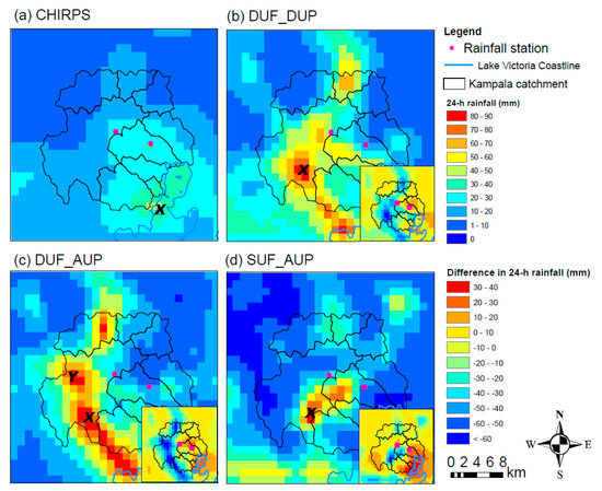
Figure 4.
24 h accumulated rainfall for (a) CHIRPS, (b) DUF_DUP, (c) DUF_AUP, and (d) SUF_AUP simulations. The insets in the bottom-right corner in (b–d) are the difference in the 24 h accumulated rainfall in the DUF_DUP, DUF_AUP, and SUF_AUP simulations from the CHIRPS observation, respectively.
3.3. Impact on 24 h Rainfall Amount
This section presents the impact of the urban landscape on 24 h rainfall amount and the inter-comparison between the three simulations (the DUF_DUP, DUF_AUP, and SUF_AUP) and benchmarked with the CHIRPS observation.
In the DUF_DUP simulation, the maximum rainfall accumulation (80 mm) is located in the southwest part of the Kampala catchment, as indicated by X in Figure 4b. Heavy rainfall amount greater than the observed rainfall (i.e., 60 mm) extends from Lake Victoria in the south/southeast to the northwest part of the Kampala catchment. In the DUF_AUP simulation, the accumulated rainfall’s spatial distribution follows a similar distribution pattern as DUF_DUP, except that the peak accumulation is higher (89 mm) at location X Figure 4c. Moreover, the location of the cluster of peak accumulation moves further to the northwest of the city (as indicated by Y in Figure 4c). In the simulation with the updated urban fraction and its parameters (SUF_AUP), the spatial rainfall pattern changed. The heavy rainfall is concentrated at the center of the city with a peak accumulation of 82 mm, as shown in location X in Figure 4d. The heavy rainfall distribution indicates the cluster of peak rainfall at three different locations (two along the coastline of Lake Victoria and one in the city center).
3.4. Impact on 2 h Rainfall Amount
The WRF model simulations are also examined to understand the precipitation event’s time evolution over the catchment by giving special attention to the timing of the observed event. Based on the Automatic Weather Station data, we know that the 25 June 2012 rainfall event lasted for two hours, from 11:10 UTC to 12:50 UTC, and we use this duration as a reference for the time evolution analysis. Figure 5 shows the cumulative rainfall curves for the observation and three WRF simulations at the AWS location. For all simulations, the event’s start is very close to the observation (i.e., about +/− 30 min), which is an outstanding result given that rainfall is highly erratic. However, all simulations do not adequately capture the end duration and time to the peak. Compared to observations, the modeled storms start a half-hour earlier for SUF_AUP and a half-hour later for DUF_DUP and DUF_AUP simulations. The time to peak (the time at the steepest slope attain) is about an hour after the observation for both DUF_DUP and DUF_AUP simulations. In the SUF_AUP simulation, the time to peak coincides well with the observed event but with a lower rain rate per minute. The result is the cumulative rainfall for the duration equivalent to the observation at the AWS location. However, due to the spatial and temporal variability of the simulated rainfall event, the analysis for a longer duration and also the analysis at different gridcell can result in a different outcome. For example, the 2 h accumulated rainfall of about 60–70 mm is simulated by all three simulations but at different locations than the AWS (see Figure 6).
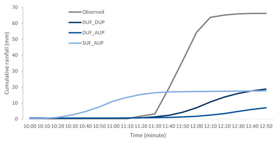
Figure 5.
Cumulative rainfall curves for observation and three WRF simulations at the AWS location. Gridcell-rainfall curves for the DUF_DUP, DUF_AUP, and SUF_AUP simulations are shown in three-hour time windows from 10:00 to 12:50, equivalent to the observation at the AWS location. The 2 h rainfall analysis focuses on the duration between 11:00 to 12:50, where the maximum peak intensity was captured by AWS observation.
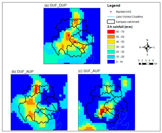
Figure 6.
2 h accumulated rainfall distribution for model simulations for the period of 11:00–12:50 UTC on 25 June 2012 (the same period as the observed rainfall using AWS in Kampala): (a) DUF_DUP, (b) DUF_AUP, and (c) SUF_AUP simulations.
The spatial distribution of the 2 h rainfall over the catchment is examined in Figure 6. In the same period of two hours, from 11:00 to 12:50, in the DUF_DUP simulation, the cluster of maximum rainfall accumulation (61 mm) is located to the southeast of the Kampala catchment area (i.e., on the edge of the catchment boundary) and extended further to the northwest of the catchment boundary. In the DUF_AUP simulation, the pattern of rainfall distribution over the catchment is similar to that of the DUF_DUP, but the maximum rainfall accumulation (72 mm) is located in the northwest of the catchment area. In the simulation in which an updated urban fraction is used (SUF_AUP simulation), the rainfall pattern is different, with a single maximum rainfall accumulation (75 mm) located in the city center. Moreover, with an updated urban fraction, the total volume of rainfall over the urban catchment is less than when using the default urban fraction. The results suggest that in addition to updated urban parameters, the change in the urban fraction (i.e., changes the intensity of urban fraction and urban extent) alters the amount, structure, and propagation of high-intensity rainfall over the city. Moreover, compared to the 24 h rainfall analysis, the pattern and location of the simulated maximum rainfall clusters for 2 h are similar to that of 24 h. However, the amount is less in the case of a 2 h duration. For instance, in the case of a 2 h duration, the maximum rainfall accumulation is reduced by 17 mm for DUF_AUP and 7 mm for SUF_AUP simulation. The reduction in rainfall amount for a 2 h duration is mainly due to temporal variability of the simulated rainfall, which is linked to the more prolonged instability in the atmosphere.
A comparison of DUF_AUP and SUF_AUP simulations with the DUF_DUP simulation over the catchment represents the impact of urban setting changes (Figure 7). The figure presents the subtraction of the DUF_DUP simulation from the two experiments, as the DUF_DUP is the reference against which we compare. The red color in the figure shows where the simulation with the experiments produces more rainfall, while the blue color gives the places the simulation with the default urban landscape produces more rainfall. The average difference in accumulated rainfall between the DUF_AUP and the DUF_DUP simulations is 22 mm (Figure 7a). The negative difference of less than −30 mm is located at the Kampala catchment’s north, central, and southeast (dark blue color). In the SUF_AUP simulation, the positive accumulated rainfall difference with the DUF_DUP simulation is, on average, +14 mm, particularly in the city center and the northern part, outside the Kampala catchment boundary (Figure 7b). The negative differences of less than −30 mm are simulated at several locations, mainly in the city center, north and southeast of the catchment (dark blue color).
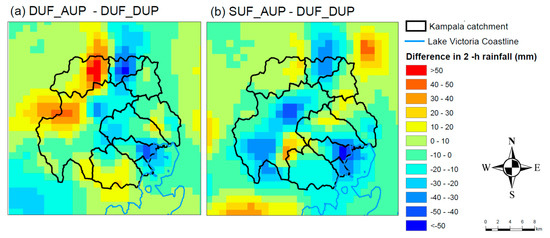
Figure 7.
2 h accumulated rainfall difference for the period of 11:00–12:50 UTC on 25 June 2012 (the same period as the observed rainfall using AWS in Kampala): subtractions of DUF_DUP simulation from (a) DUF_AUP and (b) SUF_AUP simulations.
The result also shows the inter-difference in the pattern and structure of the simulated rainfall between the DUF_AUP and SUF_AUP simulations. As shown in the figure, except in the southeast over Kampala city (red) and the furthest north of the city (blue), where the differences are the same, the patterns differ a lot elsewhere.
4. Discussion
Updating urban fractions in the WRF model can have a scientific significance in urban hydrometeorological modeling particularly to properly address the impact of urban surface heterogeneity on meteorological variables. In this research, we assessed and evaluated the impact of the updated urban fraction and urban parameters on the simulated high-intensity rainfall that can be used for proper flood hazard modeling in the urbanized and data-scarce area of Kampala, Uganda. The results indicate that the spatial distribution of the simulated event is extremely changed with the updated urban fraction. The results can be further improved by considering the effects of the explicit spatial differences in the urban morphology within the urban fraction, which is essential for a detailed analysis of hydro-meteorological processes and their impact on urban climate. This can be through comparison with the previous landcover and urban fraction development approach commonly used the World Urban Database and Access Portal Tools (WUDAPT) or Local Climate Zones (LCZ) in the WRF model. In particular, the LCZ map that the WRF model often uses was already developed for Kampala to study the variations in urban temperature and their links to health issues in the urban area [18]. Furthermore, the quality of the modeling can be improved by refining the WRF innermost domain resolution as close as that of the satellite pixel sizes to capture the actual information provided by the satellite image.
The model simulation accuracy evaluation results with the relative error (RE) index showed that the model reliably detects a cluster of maximum peak events over the city when using the updated urban fraction. When comparing the overall magnitude of error for each simulation, the SUF_AUP simulation performs better with a lower ARE score of 53%. The better performance when using an updated urban fraction is mainly due to the correct simulation of the spatial distribution of extreme grid-value rainfall events compared to when using the default urban fraction. The intercomparison between the simulations indicated that the presence of the urban landscape alters both the pattern and propagation of high-intensity rainfall over the city, mainly due to the modification of moisture transport, heat, and wind fields by the urban landscape, as indicated by [4,5].
However, there was an overall lower performance in terms of spatial distribution that was observed for all simulations, which indicates that the simulated events are spatially dislocated compared to observation. The main reason for the spatial discrepancies of the simulated events is due to a lack of sufficient observation in the urban catchment of the city for verification. Thus, two gauging stations cannot capture the simulated events across the Kampala catchment. The CHIRPS, which is the grided observed data, also indicated that the actual daily maximum rainfall in the southeastern part of the city as opposed to the WRF simulation. Overcoming the data-scarcity problem requires the installation of sufficient instruments in the catchment.
Our analysis showed that the updated urban landscape affected the location and pattern and the simulated rainfall amount over the city in two ways:
(1) Impact on location and pattern of the simulated event: The location and pattern of the simulated rainfall event are primarily affected by the updated urban parameters. Notably, unlike the DUF_DUP simulation, in the DUF_AUP simulation, the clusters of extreme rainfall concentration are increased and stretched from lake Victoria (south) to the northwest outskirt of the city. Adjusting the urban parameters (Table 2), where most values changed in favor of heat absorption by buildings during the daytime, is the main factor causing the area’s simulated rainfall displacement, which is in agreement with similar studies, for example, [7,20]. Moreover, the location and pattern of the simulated event are also affected by the updated urban fraction, as indicated in the two-hour rainfall analysis (Figure 6). Unlike the simulations that use the default urban fraction, the urbanization intensity is low in the case of the SUF_AUP simulation, which results in low drag resistance, leading to the cluster of peak events occurring in the city center. Moreover, compared to the default MODIS-based Noah urban fraction [35], the SUF_AUP simulation uses the more realistic extent of the city and fraction, resulting in a more realistic rainfall pattern compared to when using the default urban fraction, particularly in capturing the location of the event triggers the flood event. Consequently, the simulated extreme rainfall was moving south–north over the urban area. In contrast, the results of DUF_DUP and DUF_AUP simulations indicate that the cluster of extreme rainfall moves southwest, then northwest direction while decreases in rainfall amount in the urban area. Similar studies also demonstrated that the urban surface, through its surface resistance and drag force, plays a vital role in hindering the movement and speed of rainfall systems from moving toward urban areas [44,45].
(2) Impact on the amount of simulated peak event: updating urban parameters and urban fraction affected the amount of the simulated peak event. With the DUF_AUP simulation, peak rainfall event increases compared to the DUF_DUP simulation, particularly at a 24 h time scale, which is expected as the adjusted urban parameters enhance instability in the boundary layer. The presence of a high-urban fraction may act as a barrier that might split the convective cells over the city, and the high moisture in the atmosphere, as indicated by [44], may lead to an increase in the simulated rainfall. However, with SUF_AUP simulation that uses a low-urban fraction, rainfall amount is decreased compared to when using the default urban fraction (Figure 6), which is due to the reduced sensible heat flux that might lead to hindered instability in the atmosphere. The result further indicated that for the simulation with an updated urban fraction, although the considered urban extent (i.e., the area covered by urban grids) is more compared to the default urban fraction (Figure 3), the cluster of simulated heavy rainfall is fewer. This result implies that urban land surface heterogeneities are essential in affecting the mechanisms leading to the amount and spatial distribution of high-intensity rainfall events.
In the end, it is essential to outline some limitations to using the current procedure in the WRF model. One of the limitations is the stretched urban grid values created due to the resampling of the Landsat urban fraction from 30 m resolution to the model’s 1 km resolution. This shrinks the original grid values that represent high-intensity resident areas into grid values that resample more of low-intensity urban areas. Future studies further refining the WRF downscaling into high resolution, for instance, 250 m, will reduce the limitation introduced by rescaling grids. Another issue worth mentioning is that this study applied the current procedure in a single city using a single rainfall event. Future studies that will consider a greater number of rainfall events in the different urban areas can further strengthen the simulation results.
5. Conclusions
The mesoscale WRF model’s standard representation of the urban areas is often not representative of specific cities. Efforts have been made to incorporate the satellite-driven urban fraction into the WRF model for the proper simulation of extreme rainfall over Kampala, Uganda. The main approach is to utilize the high-resolution urban fraction derived based on Landsat into WRF model configured at 1 km and compare the results with the default urban fraction. Satellite urban fraction was initially developed for urban flood modeling and then following the procedure in the WRF manual we used that for WRF modeling, and urban parameters linked to the urban fractions were adjusted based on the literature review. The 25 June 2012 rainfall event that caused a localized flood event in Kampala was selected for this study. Three simulations were compared: first, with the default settings for urban fraction and its parameters (DUF_DUP); second, the simulation adjusting only the urban parameters (DUF_AUP); and finally, the simulation implementing the new urban fraction in combination with adjusted urban parameters (SUF_AUP). The peak rainfall and its spatial distribution over the Kampala catchment were evaluated using observed data from two gauging stations and the CHIRPS satellite precipitation dataset.
The results indicated benefits in several aspects of using the updated urban fraction over the default urban fraction. Mainly, the updated urban fraction represents the correct position and extent of the city leading to changes in storm structure, evolution and intensity). The results of this research indicate that the updated urban fraction in the WRF model based on the Landsat image is valuable information for the proper simulation of a high-intensity convective storm.
Compared to the observation, the spatial distribution and timing of convective storms are well captured by the WRF model when using the updated urban fraction. However, with all simulations, the WRF model overestimates rainfall compared to the CHIRPS and underestimates compared to gridcell values at gauging stations. The discrepancies between the model simulations and the CHIRPS observations are the known limitation of CHIRPS in capturing the maximum rainfall amount. Additionally, due to the absence of a dense urban gauging station network, there is no proper spatio-temporal record of the rainfall event over the city. Based on the available observations, the SUF_AUP simulation with a more realistic urban fraction and adjusted urban parameters shows relatively better performance with the lowest ARE score compared to the other two simulations.
To assess the impact of the updated urban landscape on the simulated rainfall, we analyzed rainfall distribution and amount for 24 h to understand the impact on the simulated daily rainfall and 2 h for which flood hazards occurred. Our results showed that the WRF model configuration with default urban fraction produces more peak rainfall amounts over the city with its spatial distribution covering wider areas. In contrast, the updated urban fraction has less cluster of peak rainfall events with less spatial distribution coverage within the urban catchment boundary. The results indicated benefits in several aspects of using the updated urban fraction over the default urban fraction. Mainly, the updated urban fraction represents the correct position and extent of the city that produces peak rainfall amount close to the observation. Moreover, the updated urban fraction represents the correct urban intensity that leads to less effect on the simulated rainfall. This study demonstrated that the explicit use of the satellite-derived urban fraction for NWP modeling is advantageous over the standard urban classification, mainly in two aspects: First, it represents the correct extent and position of the urban area, and second, it is possible to produce a future prediction of urbanization and then used in the NWP model for future impact assessment and local climate study. Thus, the study contributes to the emerging understanding of the usability of the high-resolution urban fractions from the remote sensing image in the NWP model to properly account for the impact of urban heterogeneity on extreme rainfall events. Moreover, the proper updating of land-use/land cover information in the NWP model contributes to improving model forecasting ability, particularly for the localized early-warning system.
Author Contributions
Conceptualization, Y.U.; methodology, Y.U. and J.E.; software, Y.U., J.E., and G.-J.S.; validation, Y.U.; formal analysis, Y.U.; investigation, Y.U.; resources, J.E. and V.J.; data curation, Y.U.; writing—original draft preparation, Y.U.; writing—review and editing, Y.U., G.-J.S., and J.E.; visualization, Y.U.; supervision, J.E. and V.J.; project administration, V.J.; funding acquisition, J.E. and V.J. All authors have read and agreed to the published version of the manuscript.
Funding
This research was conducted under the regular research program at the University of Twente.
Data Availability Statement
Data will be made available on request.
Acknowledgments
We would like to express our thanks to the University of Twente for funding this research. The authors would also like to thank Gemechu Fanta and Reinder Ronda for their support on managing and adjusting the urban fraction and vegetation cover fraction in the WRF model.
Conflicts of Interest
The authors declare no conflict of interest.
References
- Wang, H.; Hu, Y.; Guo, Y.; Wu, Z.; Yan, D. Urban flood forecasting based on the coupling of numerical weather model and stormwater model: A case study of Zhengzhou city. J. Hydrol. Reg. Stud. 2022, 39, 100985. [Google Scholar] [CrossRef]
- Umer, Y.; Jetten, V.; Ettema, J.; Lombardo, L. Application of the WRF model rainfall product for the localized flood hazard modeling in a data-scarce environment. Nat. Hazards 2022, 111, 1813–1844. [Google Scholar] [CrossRef]
- Umer, Y.; Ettema, J.; Jetten, V.; Steeneveld, G.J.; Ronda, R. Evaluation of the WRF Model to Simulate a High-Intensity Rainfall Event over Kampala, Uganda. Water 2021, 13, 873. [Google Scholar] [CrossRef]
- Paul, S.; Ghosh, S.; Mathew, M.; Devanand, A.; Karmakar, S.; Niyogi, D. Increased spatial variability and intensification of extreme monsoon rainfall due to urbanization. Sci. Rep. 2018, 8, 3918. [Google Scholar] [CrossRef] [PubMed]
- Ryu, Y.-H.; Smith, J.A.; Bou-Zeid, E.; Baeck, M.L. The influence of land surface heterogeneities on heavy convective rainfall in the Baltimore–Washington metropolitan area. Mon. Weather Rev. 2016, 144, 553–573. [Google Scholar] [CrossRef]
- Dai, J.; Wang, X.; Dai, W.; Chang, M. The impact of inhomogeneous urban canopy parameters on meteorological conditions and implication for air quality in the Pearl River Delta region. Urban Clim. 2019, 29, 100494. [Google Scholar] [CrossRef]
- Wouters, H.; Demuzere, M.; Blahak, U.; Fortuniak, K.; Maiheu, B.; Camps, J.; Tielemans, D.; Van Lipzig, N. The efficient urban canopy dependency parametrization (SURY) v1. 0 for atmospheric modelling: Description and application with the COSMO-CLM model for a Belgian summer. Geosci. Model Dev. 2016, 9, 3027–3054. [Google Scholar] [CrossRef]
- Stewart, I.D.; Oke, T.R. Local climate zones for urban temperature studies. Bull. Am. Meteorol. Soc. 2012, 93, 1879–1900. [Google Scholar] [CrossRef]
- Chen, F.; Kusaka, H.; Bornstein, R.; Ching, J.; Grimmond, C.; Grossman-Clarke, S.; Loridan, T.; Manning, K.W.; Martilli, A.; Miao, S. The integrated WRF/urban modelling system: Development, evaluation, and applications to urban environmental problems. Int. J. Climatol. 2011, 31, 273–288. [Google Scholar] [CrossRef]
- Pathirana, A.; Denekew, H.B.; Veerbeek, W.; Zevenbergen, C.; Banda, A.T. Impact of urban growth-driven landuse change on microclimate and extreme precipitation—A sensitivity study. Atmos. Res. 2014, 138, 59–72. [Google Scholar] [CrossRef]
- Sati, A.P.; Mohan, M. Impact of urban sprawls on thunderstorm episodes: Assessment using WRF model over central-national capital region of India. Urban Clim. 2021, 37, 100869. [Google Scholar] [CrossRef]
- Shepherd, J.M.; Burian, S.J. Detection of Urban-Induced Rainfall Anomalies in a Major Coastal City. Earth Interact. 2003, 7, 1–17. [Google Scholar] [CrossRef]
- Salamanca, F.; Martilli, A.; Tewari, M.; Chen, F. A study of the urban boundary layer using different urban parameterizations and high-resolution urban canopy parameters with WRF. J. Appl. Meteorol. Climatol. 2011, 50, 1107–1128. [Google Scholar] [CrossRef]
- Yang, L.; Smith, J.; Niyogi, D. Urban Impacts on Extreme Monsoon Rainfall and Flooding in Complex Terrain. Geophys. Res. Lett. 2019, 46, 5918–5927. [Google Scholar] [CrossRef]
- Brousse, O.; Martilli, A.; Foley, M.; Mills, G.; Bechtel, B. WUDAPT, an efficient land use producing data tool for mesoscale models? Integration of urban LCZ in WRF over Madrid. Urban Clim. 2016, 17, 116–134. [Google Scholar] [CrossRef]
- Alexander, P.J.; Bechtel, B.; Chow, W.T.L.; Fealy, R.; Mills, G. Linking urban climate classification with an urban energy and water budget model: Multi-site and multi-seasonal evaluation. Urban Clim. 2016, 17, 196–215. [Google Scholar] [CrossRef]
- Hu, C.; Fung, K.Y.; Tam, C.-Y.; Wang, Z. Urbanization Impacts on Pearl River Delta Extreme Rainfall Sensitivity to Land Cover Change Versus Anthropogenic Heat. Earth Space Sci. 2021, 8, e2020EA001536. [Google Scholar] [CrossRef]
- Brousse, O.; Georganos, S.; Demuzere, M.; Vanhuysse, S.; Wouters, H.; Wolff, E.; Linard, C.; Nicole, P.-M.; Dujardin, S. Using local climate zones in Sub-Saharan Africa to tackle urban health issues. Urban Clim. 2019, 27, 227–242. [Google Scholar] [CrossRef]
- Perez Molina, E. Spatial Planning, Growth, and Flooding: Contrasting Urban Processes in Kigali and Kampala. Ph.D. Thesis, University of Twente, Enschede, The Netherlands, 2019. [Google Scholar]
- Umer, Y. Advances in Localized Flood Hazard Modelling in Urbanized and Data-Scare Areas. Ph.D. Thesis, University of Twente, Enschede, The Netherlands, 2022. [Google Scholar]
- Sliuzas, R.; Flacke, J.; Jetten, V. Modelling urbanization and flooding in Kampala, Uganda. In Proceedings of the Network-Association of European Researchers on Urbanisation in the South (N-AERUS) XIV, Enschede, The Netherlands, 12–14 September 2013. [Google Scholar]
- Funk, C.; Peterson, P.; Landsfeld, M.; Pedreros, D.; Verdin, J.; Shukla, S.; Husak, G.; Rowland, J.; Harrison, L.; Hoell, A. The climate hazards infrared precipitation with stations—A new environmental record for monitoring extremes. Sci. Data 2015, 2, 150066. [Google Scholar] [CrossRef]
- Diem, J.E.; Konecky, B.L.; Salerno, J.; Hartter, J. Is equatorial Africa getting wetter or drier? Insights from an evaluation of long-term, satellite-based rainfall estimates for western Uganda. Int. J. Climatol. 2019, 39, 334–3347. [Google Scholar] [CrossRef]
- Cattani, E.; Merino, A.; Guijarro, J.; Levizzani, V. East Africa rainfall trends and variability 1983–2015 using three long-term satellite products. Remote Sens. 2018, 10, 931. [Google Scholar] [CrossRef]
- Anyah, R.O. Modeling the Variability of the Climate System over Lake Victoria Basin; North Carolina State University: Raleigh, NC, USA, 2005. [Google Scholar]
- Sun, X.; Xie, L.; Semazzi, F.; Liu, B. Effect of lake surface temperature on the spatial distribution and intensity of the precipitation over the Lake Victoria basin. Mon. Weather Rev. 2015, 143, 1179–1192. [Google Scholar] [CrossRef]
- Pérez-Molina, E.; Sliuzas, R.; Flacke, J.; Jetten, V. Developing a cellular automata model of urban growth to inform spatial policy for flood mitigation: A case study in Kampala, Uganda. Comput. Environ. Urban Syst. 2017, 65, 53–65. [Google Scholar] [CrossRef]
- Powers, J.G.; Klemp, J.B.; Skamarock, W.C.; Davis, C.A.; Dudhia, J.; Gill, D.O.; Coen, J.L.; Gochis, D.J.; Ahmadov, R.; Peckham, S.E. The weather research and forecasting model: Overview, system efforts, and future directions. Bull. Am. Meteorol. Soc. 2017, 98, 1717–1737. [Google Scholar] [CrossRef]
- Liu, J.; Bray, M.; Han, D. Sensitivity of the Weather Research and Forecasting (WRF) model to downscaling ratios and storm types in rainfall simulation. Hydrol. Process. 2012, 26, 3012–3031. [Google Scholar] [CrossRef]
- Hersbach, H.; Bell, B.; Berrisford, P.; Hirahara, S.; Horányi, A.; Muñoz-Sabater, J.; Nicolas, J.; Peubey, C.; Radu, R.; Schepers, D. The ERA5 global reanalysis. Q. J. R. Meteorol. Soc. 2020, 146, 1999–2049. [Google Scholar] [CrossRef]
- Martilli, A.; Clappier, A.; Rotach, M.W. An urban surface exchange parameterisation for mesoscale models. Bound.-Layer Meteorol. 2002, 104, 261–304. [Google Scholar] [CrossRef]
- Salamanca, F.; Krpo, A.; Martilli, A.; Clappier, A. A new building energy model coupled with an urban canopy parameterization for urban climate simulations—Part I. Formulation, verification, and sensitivity analysis of the model. Theor. Appl. Climatol. 2010, 99, 331. [Google Scholar] [CrossRef]
- Kusaka, H.; Kondo, H.; Kikegawa, Y.; Kimura, F. A simple single-layer urban canopy model for atmospheric models: Comparison with multi-layer and slab models. Bound.-Layer Meteorol. 2001, 101, 329–358. [Google Scholar] [CrossRef]
- Song, J.; Wang, Z.-H. Interfacing the urban land–atmosphere system through coupled urban canopy and atmospheric models. Bound.-Layer Meteorol. 2015, 154, 427–448. [Google Scholar] [CrossRef]
- Ran, L.; Gilliam, R.; Binkowski, F.S.; Xiu, A.; Pleim, J.; Band, L. Sensitivity of the Weather Research and Forecast/Community Multiscale Air Quality modeling system to MODIS LAI, FPAR, and albedo. J. Geophys. Res. Atmos. 2015, 120, 8491–8511. [Google Scholar] [CrossRef]
- Wang, W.; Bruyere, C.; Duda, M.; Dudhia, J.; Gill, D.; Kavulich, M.; Keene, K.; Lin, H.-C.; Michalakes, J.; Rizvi, S. User’s Guides for the Advanced Research WRF (ARW) Modeling System; Version 3; National Center For Atmospheric Research Mesoscale and Microscale: Boulder, CO, USA, 2018. [Google Scholar]
- Gilliam, R.C.; Pleim, J.E. Performance assessment of new land surface and planetary boundary layer physics in the WRF-ARW. J. Appl. Meteorol. Climatol. 2010, 49, 760–774. [Google Scholar] [CrossRef]
- Cai, M.; Ren, C.; Xu, Y.; Lau, K.K.-L.; Wang, R. Investigating the relationship between local climate zone and land surface temperature using an improved WUDAPT methodology—A case study of Yangtze River Delta, China. Urban Clim. 2018, 24, 485–502. [Google Scholar] [CrossRef]
- Oliveros, J.M.; Vallar, E.A.; Galvez, M.C.D. Investigating the Effect of Urbanization on Weather Using the Weather Research and Forecasting (WRF) Model: A Case of Metro Manila, Philippines. Environments 2019, 6, 10. [Google Scholar] [CrossRef]
- Skamarock, W.C.; Klemp, J.B.; Dudhia, J.; Gill, D.O.; Barker, D.M.; Wang, W.; Powers, J.G. A Description of the Advanced Research WRF Version 2; National Center for Atmospheric Research Boulder Co Mesoscale and Microscale Meteorology Division: Boulder, CO, USA, 2005. [Google Scholar]
- Wang, W.; Barker, D.; Bray, J.; Bruyere, C.; Duda, M.; Dudhia, J.; Gill, D.; Michalakes, J. User’s Guide for Advanced Research WRF (ARW) Modeling System Version 3; Mesoscale and Microscale Meteorology Division–National Center for Atmospheric Research (MMM-NCAR): Boulder, CO, USA, 2007. [Google Scholar]
- Guide, W.U. Chapter 3: WRF Preprocessing System (WPS). Land Use and Soil Categories in the Static Data. 2009. Available online: http://www.2.mmm.ucar.edu/wrf/users/docs/user_guide_V3/users_guide_chap3.htm (accessed on 1 March 2014).
- Tian, J.; Liu, J.; Yan, D.; Li, C.; Yu, F. Numerical rainfall simulation with different spatial and temporal evenness by using a WRF multiphysics ensemble. Nat. Hazards Earth Syst. Sci. 2017, 17, 563–579. [Google Scholar] [CrossRef]
- Miao, S.; Chen, F.; Li, Q.; Fan, S. Impacts of urban processes and urbanization on summer precipitation: A case study of heavy rainfall in Beijing on 1 August 2006. J. Appl. Meteorol. Climatol. 2011, 50, 806–825. [Google Scholar] [CrossRef]
- Zhang, Y.; Miao, S.; Dai, Y.; Bornstein, R. Numerical simulation of urban land surface effects on summer convective rainfall under different UHI intensity in Beijing. J. Geophys. Res. Atmos. 2017, 122, 7851–7868. [Google Scholar] [CrossRef]
Disclaimer/Publisher’s Note: The statements, opinions and data contained in all publications are solely those of the individual author(s) and contributor(s) and not of MDPI and/or the editor(s). MDPI and/or the editor(s) disclaim responsibility for any injury to people or property resulting from any ideas, methods, instructions or products referred to in the content. |
© 2023 by the authors. Licensee MDPI, Basel, Switzerland. This article is an open access article distributed under the terms and conditions of the Creative Commons Attribution (CC BY) license (https://creativecommons.org/licenses/by/4.0/).