Water Level Forecasting in Tidal Rivers during Typhoon Periods through Ensemble Empirical Mode Decomposition

Abstract

In this study, a novel model that performs ensemble empirical mode decomposition (EEMD) and stepwise regression was developed to forecast the water level of a tidal river. Unlike more complex hydrological models, the main advantage of the proposed model is that the only required data are water level data. EEMD is used to decompose water level signals from a tidal river into several intrinsic mode functions (IMFs). These IMFs are then used to reconstruct the ocean and stream components that represent the tide and river flow, respectively. The forecasting model is obtained through stepwise regression on these components. The ocean component at a location 1 h ahead can be forecast using the observed ocean components at the downstream gauging stations, and the corresponding stream component can be forecast using the water stages at the upstream gauging stations. Summing these two forecasted components enables the forecasting of the water level at a location in the tidal river. The proposed model is conceptually simple and highly accurate. Water level data collected from gauging stations in the Tanshui River in Taiwan during typhoons were used to assess the feasibility of the proposed model. The water level forecasting model accurately and reliably predicted the water level at the Taipei Bridge gauging station.

1. Introduction

An estuary is a transition zone with complex flow conditions in which a river enters the ocean. Complex factors contribute to the water level in tidal rivers; the water level is affected by not only the upstream river discharge but also ocean tides [1]. The water level in a tidal river changes because of the interaction between riverine and marine factors. Because of the rotation of the Earth and the varying strength of the gravitational pull from the Moon and Sun, the water level varies quasiperiodically every 12.25 h or twice every lunar day. [2]. Longer-period effects from storms and seasonal fluctuations influence salinity. Flooding from the upstream basin can alter the salinity profile and interrupt the tidal cycle [3]. A major climate factor affecting estuaries is wind; wind creates waves, which affect water circulation and the mixing of fresh and seawater [4]. Upon circulation and mixing, the 2% difference in the densities of fresh and seawater creates a pressure gradient in the horizontal direction that affects the water flow [5]. This density difference is largely caused by differences in temperature and salinity; however, salinity is by far the dominant factor affecting tidal river dynamics [6]. Considering all the aforementioned information, accounting for all physical processes in tidal rivers is challenging. These hydrological processes are complex, have mutual interactions, and are the driving forces [7] for other sedimentological, biological, and chemical processes. It is not easy to develop a model that can deal with all hydrological processes in tidal rivers. No simple conventional method can accurately forecast the discharge and water level in tidal rivers.

Because of the extremely unsteady flow conditions of tidal rivers or estuaries, forecasting their water levels is a difficult task. Theoretical and empirical approaches are commonly used to perform this task. The hydrological processes in a tidal river are unique, and the water level in a tidal river is continually changing because of the interactions of riverine and marine processes. The factors affecting water levels include the shape of the tidal river, astronomical tides, wind, salinity, temperature, sediment, flood, storm surge, and other factors that are too complex to model directly. Consequently, the hydrodynamic processes of tidal rivers are complex, nonstationary, and nonlinear [8]. Many of the concepts or principles identified by modeling other watercourses have been applied to forecast water levels in tidal rivers. The theoretical approach is based on continuity, momentum, and energy equations. However, a major disadvantage of theoretical methods is that the required parameters are usually difficult to determine from the observed data; in particular, the discharge is challenging to measure [9]. Although there are lots of open-source models available for free, programming and executing a newly developed model is time-consuming and costly. Some hydraulic models apply the mass conservation and momentum principle [10,11,12] to forecast water levels and current velocities during spring and neap tidal cycles. Hydrological routing, which is a simpler technique than that of hydraulic models, uses a continuity equation combined with a storage indication curve to forecast estuary water levels [13]. These hydraulic and hydrological models usually apply numerical methods to obtain results. Artificial neural networks (ANNs) have been widely used for data mining. An ANN is a black-box technique that can be used for water resource management and modeling hydrological processes [14,15,16]. An ANN can also be applied for forecasting tidal river water levels [8,17].

The variation in the water level of tidal rivers with time can be regarded as a signal. Some methods for signal processing analysis, such as the Fourier [18,19] and wavelet [20,21] transforms, are often used to analyze historical data for forecasting tidal river or estuary water levels. The Fourier transform can only be applied to linear and stationary processes, and wavelet transforms can only be applied to linear and nonstationary processes. However, the hydrological processes in tidal rivers are nonlinear and nonstationary. A novel method of handling nonstationary and nonlinear data is the Hilbert–Huang transform (HHT), which was proposed by Huang et al. [22,23]. The HHT is a method of decomposing an original signal into many intrinsic mode functions (IMFs) with a trend. The fundamental process of the HHT is the empirical mode decomposition (EMD) or ensemble EMD (EEMD) method, which involves breaking down a signal into various IMFs. Since their introduction, the EMD and EEMD methods have rapidly grown in popularity and have been effectively applied to estuaries [24,25], oceans [26,27], and other engineering fields, including water resources [28,29].

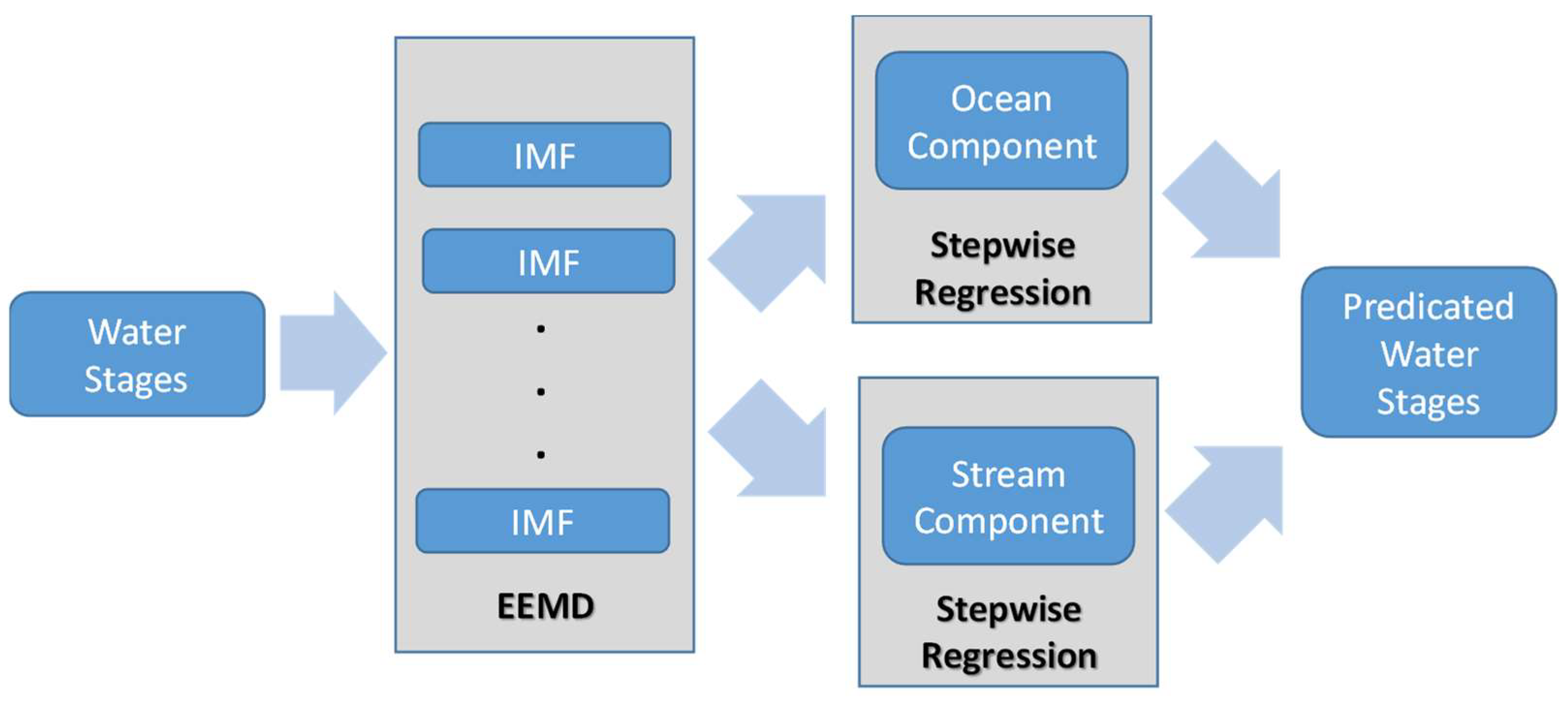
In this study, a conceptual model was developed for forecasting tidal river water levels during a flood period (Figure 1). The proposed model only requires water level data for prediction. EEMD is applied to decompose the water levels in tidal rivers into several IMFs. The IMFs decomposed through EEMD usually have a physically meaningful correspondence to physical data [30,31,32,33]. The water level in a tidal river is affected by many factors, such as tide, topography, friction, and river flow [24], in a complex manner. However, these data are difficult to obtain and thus cannot be used to develop a sophisticated model. By contrast, water level data can be easily collected. IMFs can be obtained through EEMD; however, because of a lack of data, the factors affecting IMFs cannot be determined. Therefore, the developed model was simplified by dividing IMFs into two groups: ocean and stream components. These components were used to establish regression methods for forecasting the contribution of each component to the water level. By adding the contributions from the two forecasted components, the water level in tidal rivers can be obtained. Finally, the water stages of the Tanshui River in Taiwan during typhoon periods were used as an example to demonstrate the calculation procedures and validate the reliability and accuracy of the proposed model.

2. EEMD and Stepwise Regression

2.1. EEMD Method

Huang et al. [23] proposed the EMD method, which is an intuitive and adaptive data analysis method. In EMD, basis functions are derived from the original signals. The aforementioned method directly resolves energies by using the intrinsic time scale of the original data, which are decomposed into several simple harmonic functions (i.e., IMFs) with different periodicity. An IMF is a simple oscillatory mode corresponding to a simple harmonic function and must satisfy the following two requirements. First, in the entire data set, the number of extrema and the number of zero-crossings must be equal or differ at most by 1. Second, at any point, the mean value of the envelopes defined by the local maximum and minimum is 0. Thus, EMD is used to decompose an original signal into multiple IMFs with different frequencies and a residual signal. These IMFs form a complete and nearly orthogonal basis for the original signal. An IMF can have variable amplitude and frequency along the time axis. The EMD method differs from wavelet and Fourier analysis in that the basis is not predetermined. Consequently, the characteristics of the original signal can be fully reflected. The EMD method is intuitive, direct, and self-adaptive.

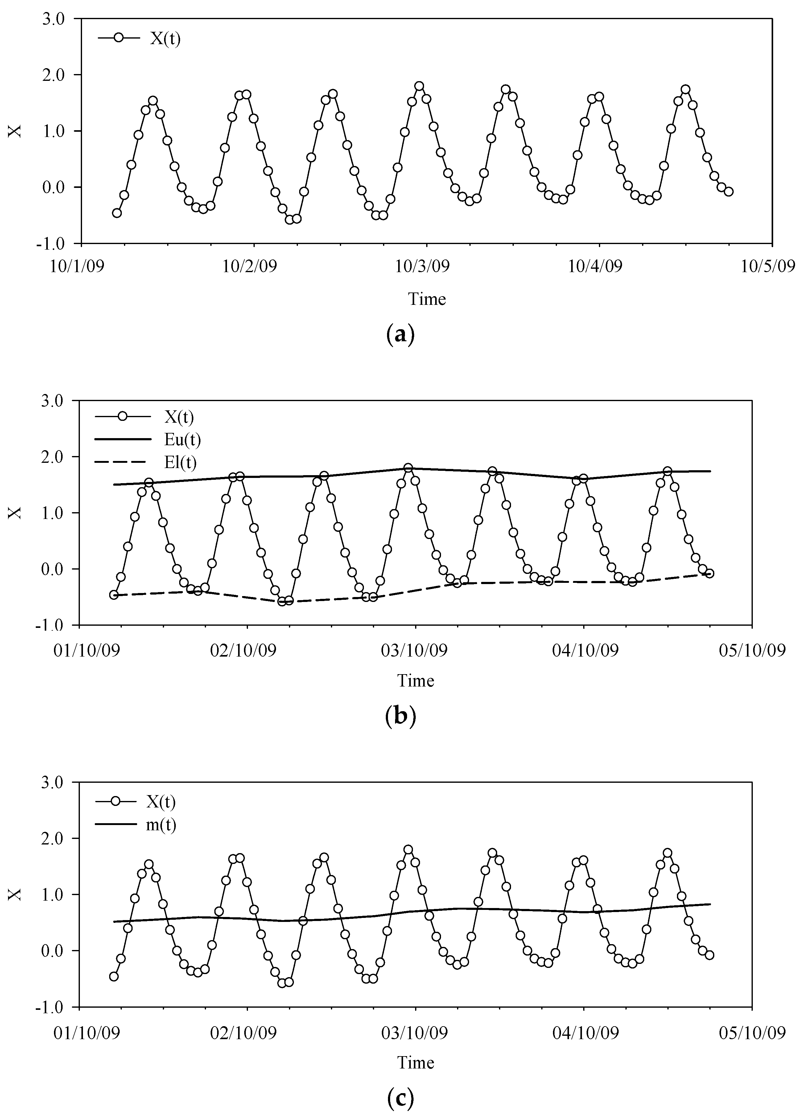
The procedure of extracting an IMF is called sifting. Figure 2 presents an example of the sifting process for the time series of water level X(t). This process involves the following steps:

A.

The local maxima and minima in X(t) are identified, as shown in Figure 2a.

B.

Cubic spline is used on the local maximum and minimum values to generate two curves approximating the envelopes, namely, the upper and lower envelopes, as displayed in Figure 2b.

C.

A mean curve is calculated from the two envelopes, as illustrated in Figure 2c. The mean is expressed as follows:

$$m\left(u\right)=\frac{E_u\left(t\right)+E_l\left(t\right)}{2}$$

(1)

where m(t) is the mean, E_u(t) is the upper envelope, and E_l(t) is the lower envelope.

A variable d(t) is defined as follows:

$$d\left(t\right)=X\left(t\right)-m\left(t\right)$$

(2)

where d(t) is the difference between X(t) and m(t). If d(t) does not meet the stopping criterion, d(t) is set as the new X(t) value, and the aforementioned steps are repeated to differentiate the extremes until d(t) reaches the stopping criterion.

An excessive number of selection cycles can reduce the physical meaning of the IMF’s instantaneous frequency and amplitude; thus, a stopping criterion must be set. The stopping criterion is based on the amplitude, energy, and phase. Common stopping criteria include the standard deviation, an S-number criterion [34], and an evaluation function [35]. In this study, the S-number criterion was used, where S is the maximum number of selection cycles. A selection cycle is terminated when the number of extreme values matches the number of zero-crossings.

The d(t) value that meets the stopping criterion is set as an IMF, namely, C_j(t), where j is a value from 1 to n. The residual R_j(t) is the new X_j+1(t) value, as expressed in the following equation:

$$R_j\left(t\right)=X_{j+1}\left(t\right)$$

(3)

EMD is then repeated to obtain additional IMFs. The final IMF n is recorded as C_j=n(t). The term X(t) represents the superposition of various IMF components (C_j(t) and R_n(t)) and is expressed as follows:

$$X\left(t\right)={\displaystyle \sum }_{j=1}^n{C}_j\left(t\right)+R_n\left(t\right)$$

(4)

In EMD, the problem of mode mixing occurs. Mode mixing is a problem in which an IMF produced through EMD decomposition contains components of different frequencies. Mode mixing is caused by intermittent signals and noise. In particular, mode mixing occurs because of unpredictable random noise contained in the original signal infiltrating the IMFs. This intermittent, irregular noise affects the determination of the upper and lower envelopes. Consequently, two signals of different time scales can be classified as one IMF, or signals of the same time scale might be separated into two IMFs. Mode mixing eliminates the physical significance of the IMF. To overcome this challenge, Wu and Huang [36] proposed the EEMD method, in which white noise is introduced to eliminate the effect of the original noise and obtain mode-consistent IMFs. EEMD is performed as follows. First, a white noise signal w_i(t) is added to the original signal to form an ensemble. Second, the ensemble is subjected to EMD decomposition into several IMFs. Third, the first and second steps are repeated by adding white noise on each time scale.

Because white noise is stochastic and uniformly distributed on every component, its effect can be eliminated as its ensemble number increases; that is, if sufficient white noise addition cycles are performed, the obtained solution approaches the true answer, and the goal of eliminating noise and mode mixing can be achieved. According to statistical theory, the influence of the added noise and its relation to the ensemble number is expressed as follows:

$${\epsilon }_n=\frac{\epsilon }{\sqrt{n}}$$

(5)

where n is the ensemble number, ε is the amplitude of the added white noise, and ε_n is the standard error. The noise-added signal based on the aforementioned relation is represented as follows:

$$X_E\left(t\right)=X\left(t\right)+\epsilon \times noise\left(t\right)$$

(6)

The signal in Equation (6) is subjected to EMD decomposition. The IMFs at different frequencies are obtained from the ensemble average of each component.

Each IMF (C_j(t)) calculated through EEMD inherits the physical meaning of the original data. Therefore, EEMD is often applied in geographic research [36]. Tidal river water level is profoundly influenced by tides. If EEMD is used for analysis, water level can be decomposed into mutually independent IMFs with corresponding frequencies. Thus, the frequency of each IMF can be compared with the tidal frequency in the studied area. If an IMF has periodicity, it is likely to be related to tides. Therefore, IMFs generated from water level data can be classified into two groups: tidal functions and flood functions. By adding all tidal IMFs, the ocean component can be obtained; similarly, the stream component can be obtained by summing the remaining IMFs.

2.2. Stepwise Regression Analysis

Stepwise regression, which is a multiple linear regression technique, is an efficient method of selecting the most useful explanatory variables. This method is a modification of forward selection. The general idea behind stepwise regression is that at each stage of selection, all model variables are evaluated using the partial F-test based on a preselected critical value.

Initially, the candidate variables are identified. Stepwise regression with forward selection begins with no variables in the regression model. Let the set of all possible variables be x₁, x₂, …, x_m. In stepwise regression, the model is initially fitted with only one variable. After fitting the variable x_i, the fit is checked using the critical F value. Models with two variables are then considered. The optimal regression model with variables x_i and x_j is selected using the F-test and is included in the model. This process continues until the F-test indicates that the inclusion of further functions is not useful, at which point a final model is obtained.

The key task in forecasting tidal river water levels involves constructing regression models for the ocean and stream components. The goal of the ocean- and stream-component regression models is to establish the relationship between the downstream and upstream water levels, respectively, and the forecasted values at the site of interest. By summing the forecasting values obtained from these two regression models, the water level of a tidal river can be predicted.

3. Study Area and Data Descriptions

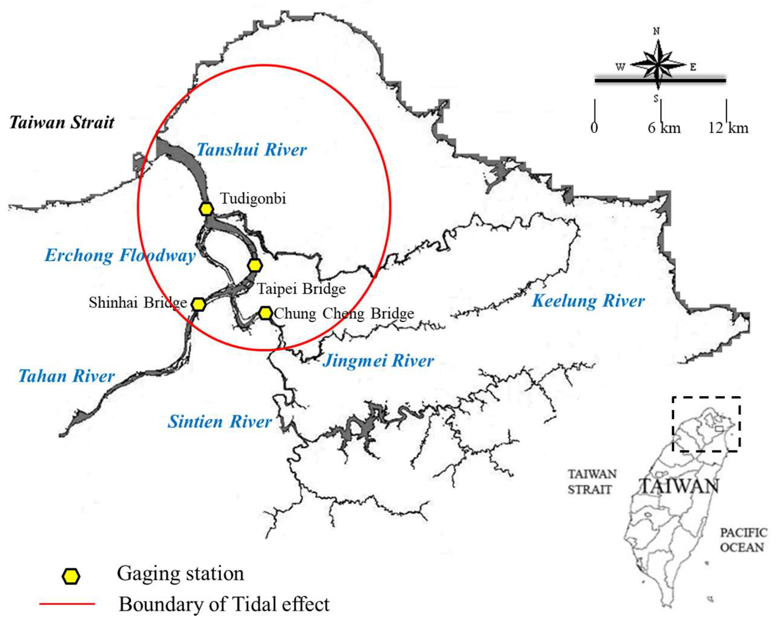
In this study, water level data from the Tanshui River in Taiwan were used to evaluate the proposed model. As illustrated in Figure 3, the tributaries of the Tanshui River include the Keelung River, Hsin-Tien River, and Dahan River. The Tanshui River is formed by the merger of the Tanhan River and Xindian River. The largest tributary of the Tanshui River is the Keelung River. The Hsin-Tien River is approximately 21 km long and runs south to north through Taipei to the Taiwan Strait. The main stream of the Tanshui River has a length of 158.7 km and drains 2575 km² in north Taiwan. It originates from a 3529 m high mountain with an average gradient of 1:122. In Figure 3, the circle denotes the tidal area of the Tanshui River [37]. Tides in the Taiwan Strait primarily comprise the four tide components O1, K1, M2, and S2; the tide level data mostly comprise the principal lunar semidiurnal constituent. Semidiurnal tides are the most influential tides in the Tanshui River. The average tide level at the river mouth gauging station is 0.03 m, with the average tide range being 2.19 m, spring tide range being 2.89 m, and maximum tide range being 3 m because of the contraction of the channel cross section and wave propagation. The difference between the two tidal ranges each day is small, and the tidal range of diurnal tides is approximately 1/5th that of semidiurnal tides.

The Tanshui River flows past the Taipei metropolitan area, which is Taiwan’s political and cultural center. Taipei, which is situated in a low-lying basin, is susceptible to flooding. A flood control system was constructed in Taipei beginning in 1970. This system includes dams, levees, pumping stations, floodways, and a warning system and is designed to withstand floods with a 200-year return period. Typically, no water flows in the Erchong Floodway on ordinary days. If extreme flooding occurs, the water from the Tahan River and Hsin-Tien River is redirected to the floodways and purged downstream in the Tanshui River. The flood warning system must accurately forecast water levels during flood periods. Therefore, gauging stations operated by the 10th River Management Office were established within the Tanshui River estuary region to collect water levels for flood routing; these stations include Tudigonbi, the Taipei Bridge on the Tanshui River, the Shinhai Bridge on the Tahan River, and the Chung Cheng Bridge on the Hsin-Tien River.

The narrowest cross section of the Tanshui River is located at the Taipei Bridge. Consequently, when flooding occurs, the velocity and water level at this spot increase considerably, which often results in serious damage. Therefore, forecasting the water level at the Taipei Bridge is an essential task for the flood warning system. In this study, EEMD was conducted to construct a water level forecasting model for flood warnings at the Taipei Bridge. The results of EEMD were used to assess the reliability and accuracy of the proposed model. Floods from the Tahan River and the Hsin-Tien River upstream of the Tanshui River and tides downstream of the Taipei Bridge affect the water level at the Taipei Bridge. Therefore, the stream component at the Taipei Bridge was forecast using data from the gauging station at the Shinhai Bridge on the Tahan River and the station at the Chung Cheng Bridge on the Hsin-Tien River, which is located upstream of the Taipei Bridge. The ocean component at the Taipei Bridge was forecast using data from the Tudigonbi station located downstream of the Taipei Bridge. Finally, by adding the forecasted stream and ocean components, the water level forecast at the Taipei Bridge was obtained.

The proposed model requires water level data for the Tudigonbi, Shinhai Bridge, and Chung Cheng Bridge stations to forecast the water level at the Taipei Bridge. The water level at each gauging station during typhoon periods differs considerably from that on ordinary days. Therefore, in this study, 15 typhoon or heavy storm events with complete water level data from 2004 to 2015 were used to establish a model for forecasting estuarine water levels. High-water data were selected as those from the period starting 1 day before the issue of a typhoon warning and ending the day after lifting the warning. A total of 10 out of the 15 events were further categorized for calibrating the proposed model; the remaining five events were used to verify the model.

Table 1. Summary description of water levels at the Taipei Bridge during typhoons.

Phase	Typhoon	Duration	Water Level (m)
			Max.	Min.
Calibration	Nock−Ten	22/10/2004–27/10/2004	1.88	−1.11
	Haitang	15/7/2005–21/7/2005	1.93	−1.34
	Matsa	2/8/2005–7/8/2005	3.62	−1.13
	Longwang	29/9/2005–4/10/2005	1.83	−1.12
	Fung−Wong	25/7/2008–30/7/2008	1.98	−1.13
	Fanapi	19/9/2010–21/9/2010	1.56	−0.91
	Saola	29/7/2012–4/8/2012	5.28	−1.09
	Soulik	10/7/2013–14/7/2013	2.88	−1.15
	Kong−Rey	26/8/2013–23/8/2013	1.68	−0.74
	Soudelor	5/8/2015–10/8/2015	5.17	−1.01
Verification	Mindulle	27/6/2004–4/7/2004	2.38	−1.58
	Kalmaegi	15/7/2008–19/7/2008	1.81	−1.12
	Sinlaku	10/9/2008–17/9/2008	3.45	−0.91
	Trami	19/8/2013–23/8/2013	2.85	−1.15
	Dujuan	26/9/2015–30/9/2015	3.78	−1.21

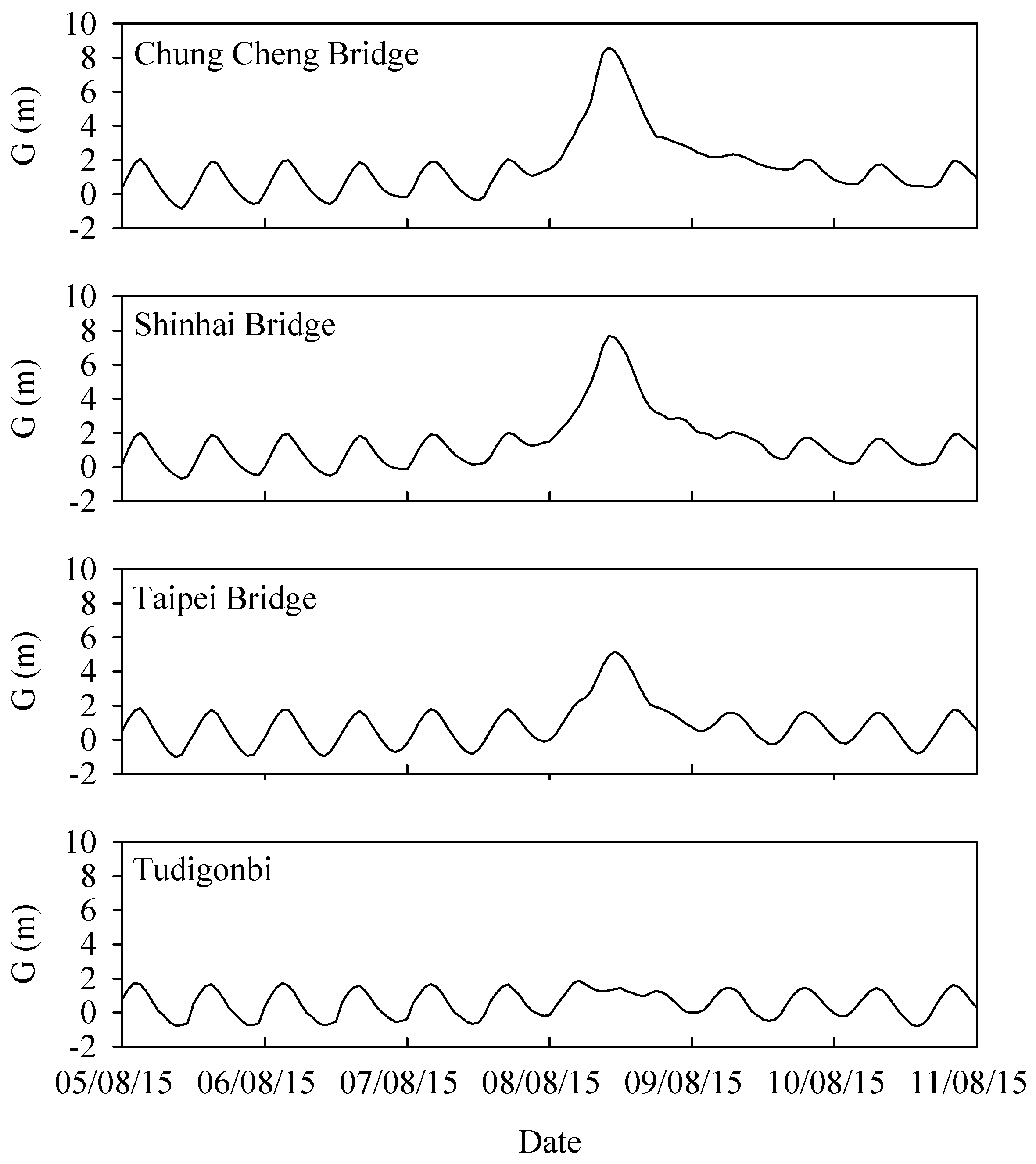
lists the starting and ending times and the highest and lowest water levels at the Taipei Bridge for each typhoon event. Figure 4 presents the water level at each gauging station during Typhoon Soudelor; all gauging stations had an atypically high water level. The water level at the Chung Cheng Bridge and Shinhai Bridge, which are located at the boundary of the tidal area, increased sharply because of flooding. The water level at the Taipei Bridge also increased; however, this increase was smaller than those at the Chung Cheng Bridge and Shinhai Bridge. The only station close to the river mouth, namely, the Tudigonbi station, also exhibited a higher water level than usual; however, the difference was small. The periodic regularity of the water level disappeared for all gauging stations.

4. Practical Applications

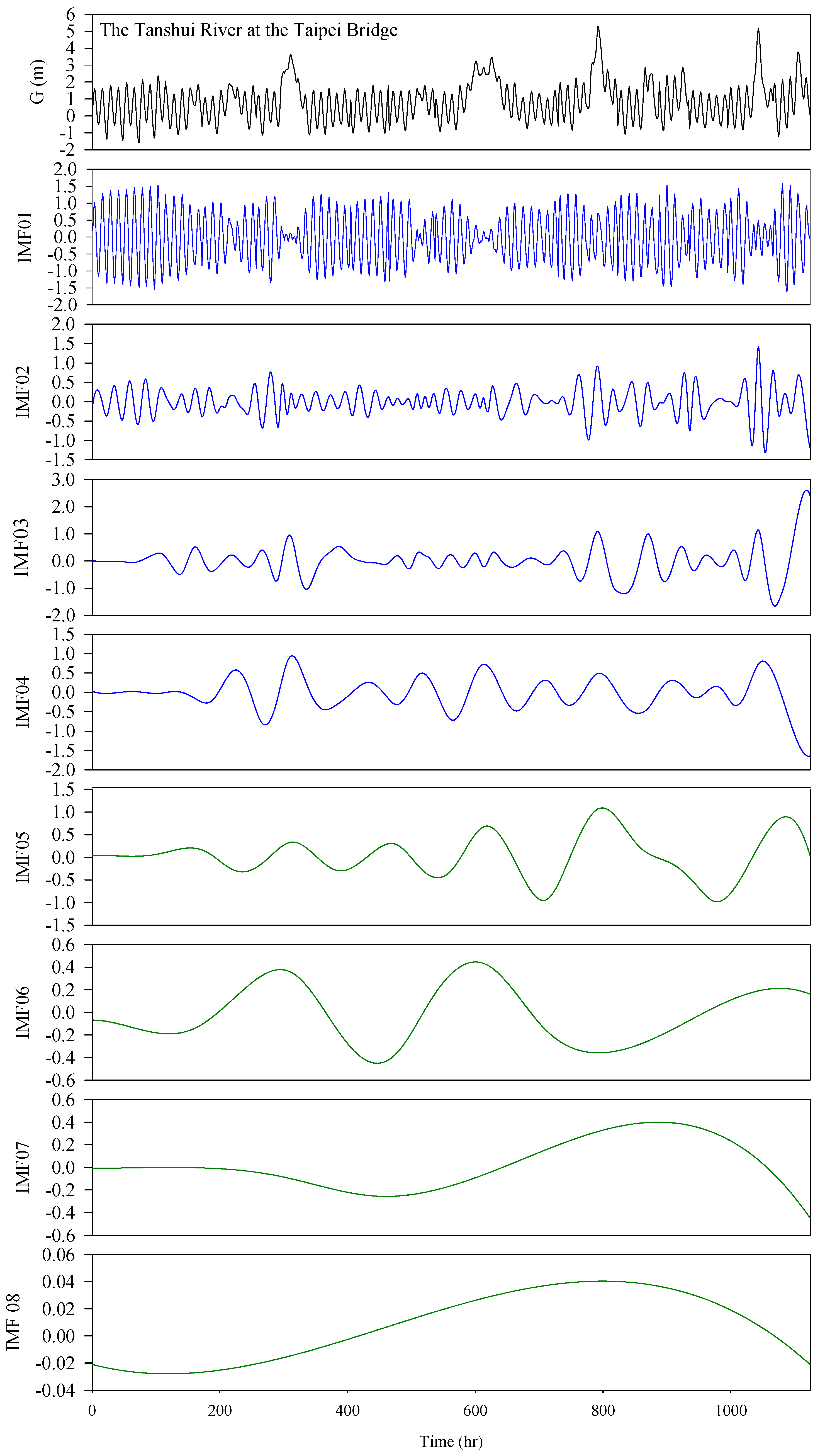
All hydrographs of the 15 events were connected, and EEMD was conducted to obtain the IMFs. The uppermost plot of Figure 5 presents the gauge height (G) at the Taipei Bridge, and the subsequent curves are represented in IMF1 to IMF8. IMF1, IMF2, IMF3, and IMF4 had periodicity; that is, these IMFs exhibited a pattern of cycles that repeat at intervals.

Table 2. Frequency (hr⁻¹) of the gauging stations.

Station	IMF1	IMF2	IMF3	IMF4	IMF5	IMF6	IMF7
Chung Cheng Bridge	0.0805	0.0805	0.0400	0.0218	0.0075	0.0049	0.0027
Shinhai Bridge	0.0805	0.0805	0.0415	0.0213	0.0098	0.0052	0.0025
Taipei Bridge	0.0805	0.0805	0.0388	0.0186	0.0100	0.0049	0.0025
Tudigonbi	0.0805	0.0805	0.0388	0.0174	0.0091	0.0049	0.0025

lists the periodicity for all IMFs at each gauging station. The frequencies (dividing the number of times an event occurs by the duration) of IMF1 and IMF2 for each station were approximately 0.0805 h⁻¹, which is similar to the M2 tidal component frequency presented in

Table 3. The classical tidal type.

Type	Characterizes	Name	Cycle (Hour/Cycle)	Frequency (hr−1)
Semidiurnal tides	K2	Lunisolar diurnal constituent	11.9672	0.0836
	S2	Principal solar semidiurnal constituent	12.0000	0.0833
	M2	Principal lunar semidiurnal constituent	12.4206	0.0805
	N2	Large lunar elliptic semidiurnal constituent	12.6583	0.0775
	2N2	Second large lunar elliptic semidiurnal constituent	12.9054	0.0790
Diurnal tides	K1	Lunisolar diurnal constituent	23.9345	0.0418
	P1	Principal solar diurnal constituent	24.0659	0.0416
	O1	Principal lunar diurnal constituent	25.8193	0.0387
	Q1	Large lunar elliptic constituent	26.8684	0.0372
Overtides	S4	Solar quarter constituent	6.0000	0.1667
	M4	Large lunar quarter constituent	6.2103	0.1610

. This result suggests that IMF1 and IMF2 represent the influences of the semidiurnal tides. The periodicity of IMF3 for all stations was close to the principal solar or lunar diurnal constituent (P₁ and O₁ in Table 3), which indicated that diurnal tides contributed to the IMF3 component. IMF5, IMF6, IMF7, and IMF8 were clearly related to the tides. Therefore, IMF1–IMF4, which exhibited periodicity, were classified as ocean components, and the remaining IMFs were classified as stream components. Thus, the following equation is obtained:

OC = IMF1 + IMF2 + IMF3 + IMF4

(7)

SC = G − OC

(8)

where OC is the ocean component and SC is the stream component.

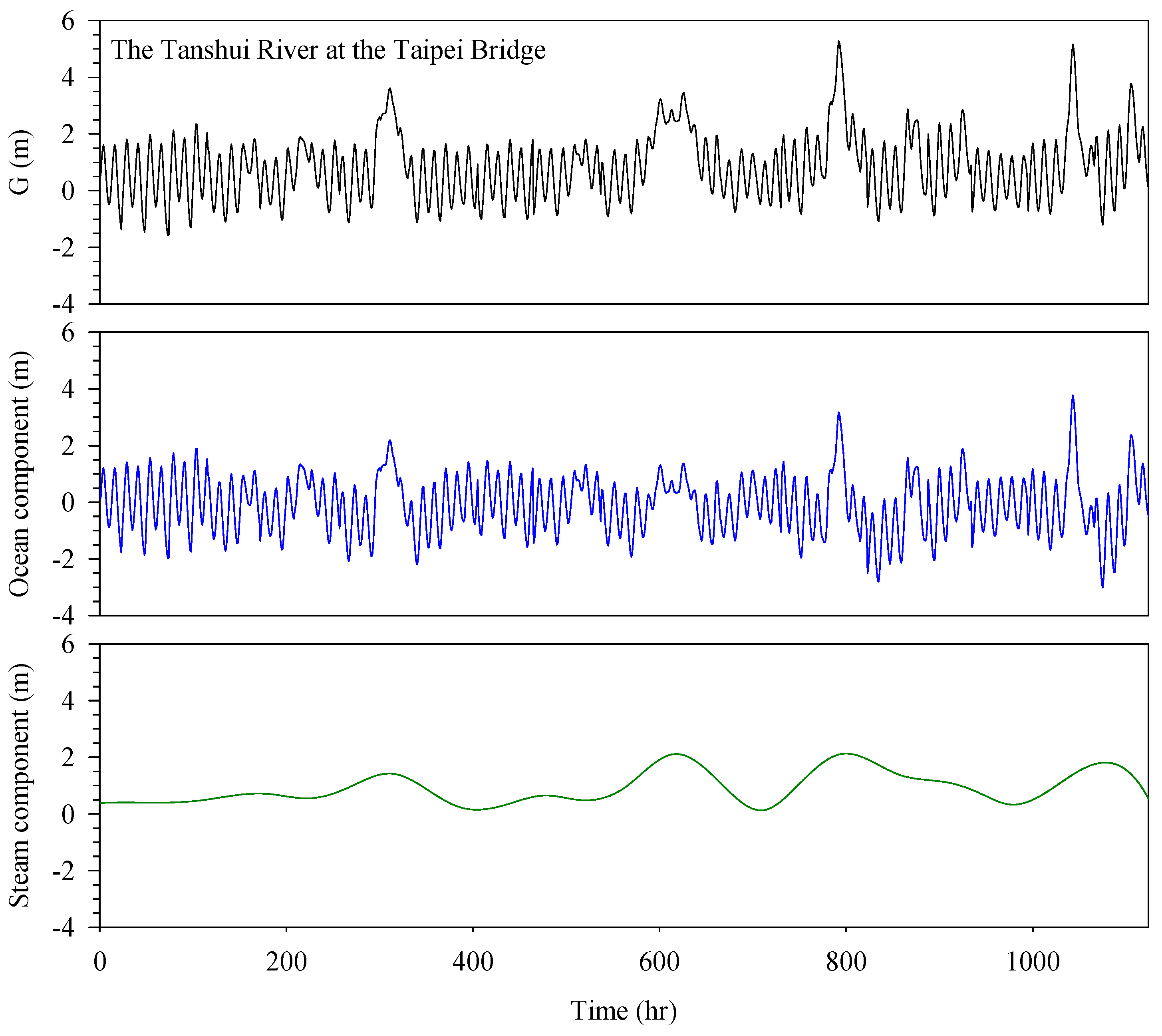
Figure 6 presents the results of the EEMD decomposition of the water level at the Taipei Bridge into ocean and stream components. The results reveal how tides and upstream discharge affect the water level at the Taipei Bridge.

The lag time of the ocean components at the Taipei Bridge is related to the tides. Therefore, the regressors for forecasting the 1 h ahead ocean component (at t + 1) are the neighboring values of the ocean component at the Taipei Bridge and Tudigonbi for up to 3 h before the event (i.e., from t − 2 to t). A suitable linear regression model is given as follows:

$$O{C}_{T, t+1}={\beta }_0+{\beta }_{1}O{C}_{T,t}+{\beta }_{2}O{C}_{T,t-1}+{\beta }_{3}O{C}_{T,t-2}+{\beta }_{4}O{C}_{D,t}+{\beta }_{5}O{C}_{D,t-1}+{\beta }_{6}O{C}_{D,t-2}$$

(9)

where OC_T and OC_D indicate the forecasted ocean components at the Taipei Bridge and Tudigonbi, respectively; the subscripts t − 2, t − 1, t, and t + 1 indicate the time; and β₀, β₁, …, β₆ are the regression coefficients. By fitting Equation (9) to the ocean component data of the calibration phase by using the stepwise regression method, the following equation is obtained:

$$O{C}_{T, t+1}=-0.004+1.791O{C}_{T,t}-0.456O{C}_{T,t-1}+0.213O{C}_{T,t-2}-1.052O{C}_{D,t-1}$$

(10)

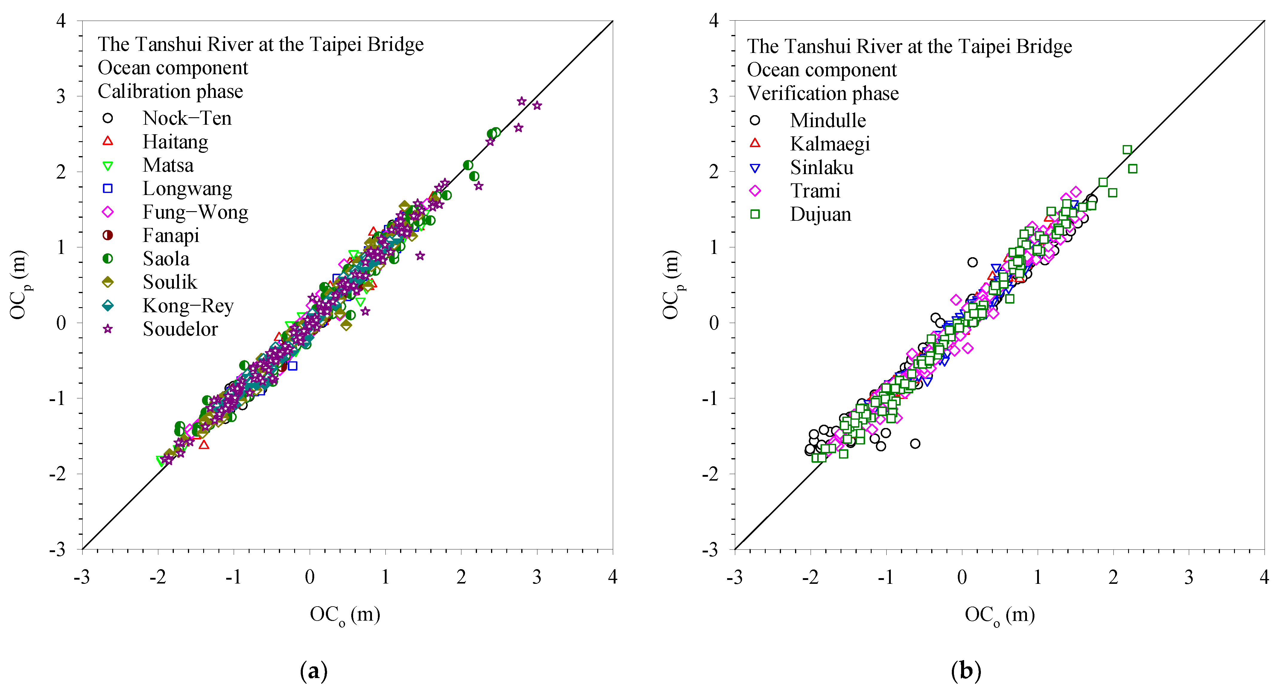
Figure 7 presents a comparison of the observed ocean component (OC_o) and forecasted ocean component (OC_p) and reveals that the water levels forecast through EEMD and stepwise regression are consistent with the observed water levels in the model calibration and verification processes. This figure also indicates that the proposed model can effectively reflect tidal dynamics.

Linear regression was conducted to forecast the stream component at the Taipei Bridge. The forecasted stream component at time t + 1 is a function of the stream components at the Chung Cheng Bridge and Shinhai Bridge at times t, t − 1, and t − 2. Stepwise regression was applied to produce the following stream component forecasting model:

$$S{C}_{T, t+1}=0.042+1.333S{C}_{C,t}-1.311S{C}_{C,t-1}+0.503S{C}_{S,t}$$

(11)

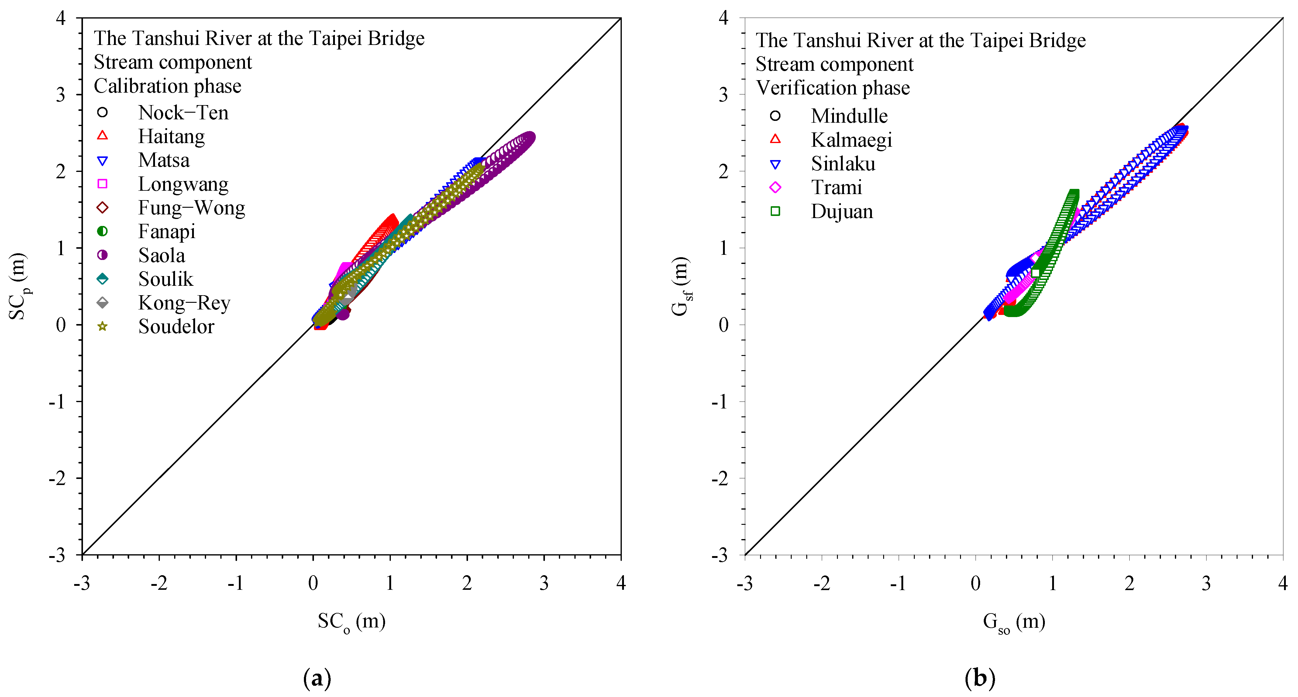
where SC_T,t+1 is the forecasted stream component of the Taipei Bridge at time t + 1; SC_C,t−1 is the stream component of the Chung Cheng Bridge at time t − 1; and SC_C,t and SC_S,t are the stream components of the Chung Cheng Bridge and Shinhai Bridge at time t, respectively. Scatter plots of the observed and forecasted stream components in the calibration and verification phases are displayed in Figure 8. The terms SC_o and SC_p denote the observed and forecasted stream components, respectively. All the data points fall on or near the line of agreement between the observed and predicted results, which indicates the accuracy of the forecasted stream components.

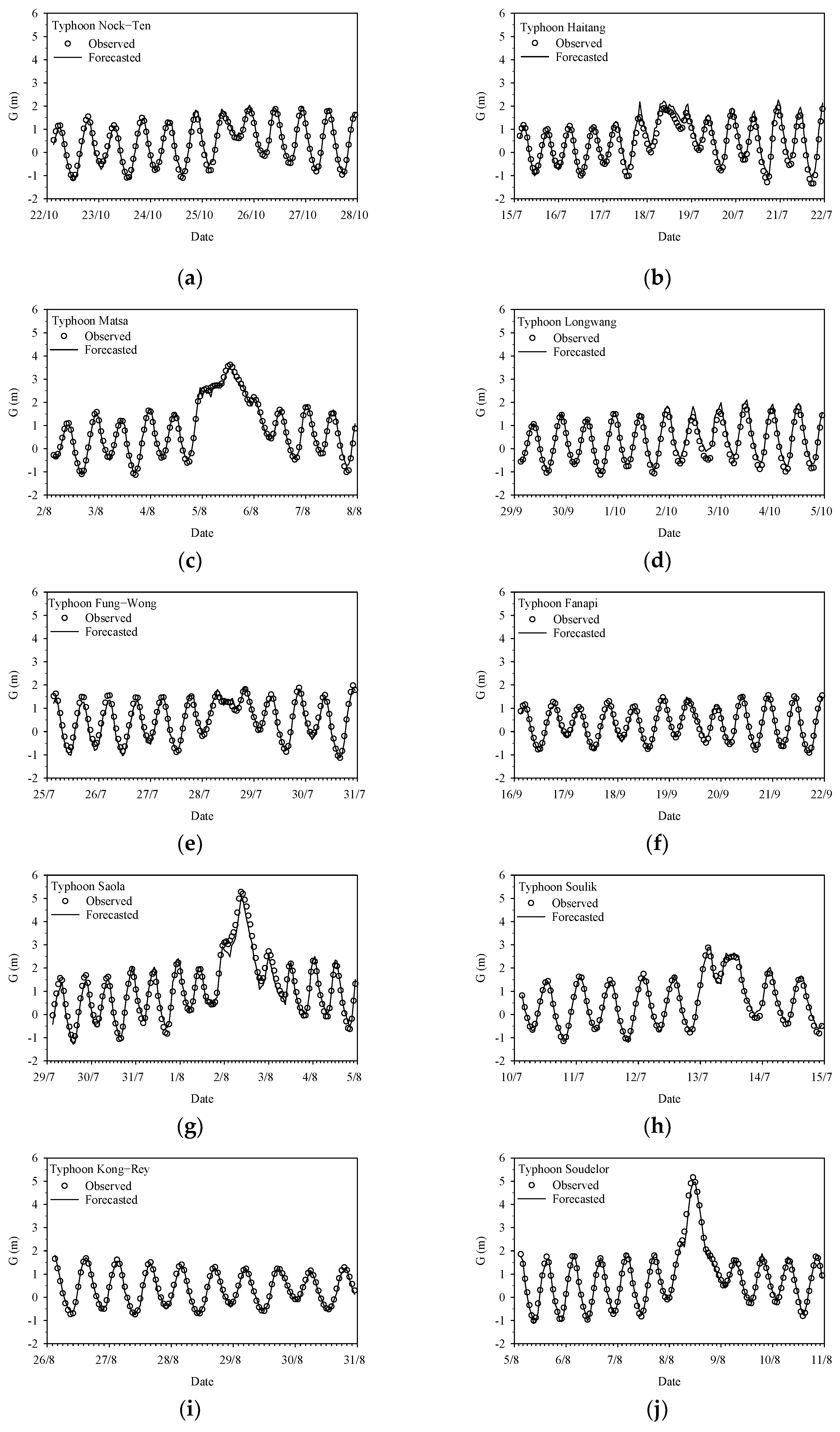
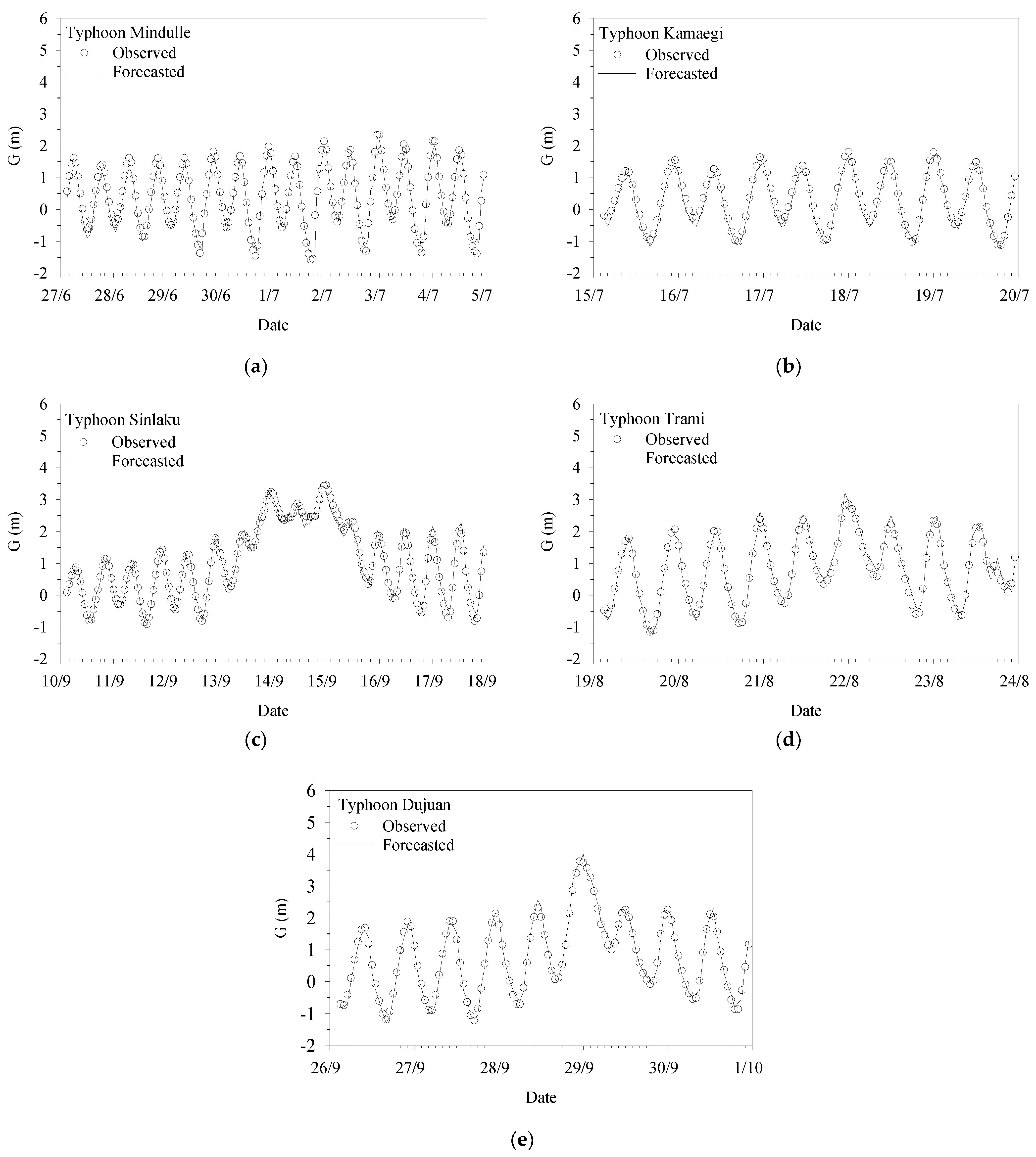
Figure 9 and Figure 10 present a comparison of the water levels forecast by the proposed model and the observed water levels in the calibration and validation phases. The forecasted water level is the sum of the forecasted ocean and stream components. The forecasted water levels of the proposed model are highly accurate. A comparison of the forecasted and observed water levels indicates that tidal amplitude, phase, and spring and neap tide modulations are accurately captured by the proposed model. Furthermore, the forecasted peaks are similar to the observed peaks. Therefore, the effect of floods on the water level in a tidal river can also be accurately forecast by the proposed EEMD model.

The quantitative metrics used for evaluating the accuracy of the proposed model were correlation coefficient (ρ) and root-mean-square error (RMSE), which are defined as follows:

$$\rho =\frac{{{\displaystyle \sum }}^{}\left(G_p-{\overline{G}}_p\right)\left(G_o-{\overline{G}}_o\right)}{\sqrt{{{\displaystyle \sum }}^{}{\left(G_p-{\overline{G}}_p\right)}^2{{\displaystyle \sum }}^{}{\left(G_o-{\overline{G}}_o\right)}^2}}$$

(12)

$$RMSE=\sqrt{\frac{{{\displaystyle \sum }}^{}{\left(G_p-G_o\right)}^2}{N}}$$

(13)

where G_p and G_o are the forecasted and observed water levels, respectively; ${\overline{G}}_p$ and ${\overline{G}}_o$ are the means of the forecasted and observed water levels, respectively; and N is the number of data sets.

Table 4. Summary of performance metrics carried out by comparing observations and forecasts.

	Phase	RMSE (m)	ρ
Ocean component	Calibration	0.10	0.986
	Verification	0.13	0.978
Stream component	Calibration	0.14	0.937
	Verification	0.12	0.969
Water level	Calibration	0.18	0.971
	Verification	0.17	0.976

lists the statistics corresponding to Figure 7, Figure 8, Figure 9 and Figure 10. All correlation coefficients are close to unity. The RMSEs are between 0.10 and 0.17 m. These values are considerably smaller than the water level range. These statistical measures indicate that the proposed model is accurate, and its predictions are consistent with the observations; thus, this model can effectively forecast the water level in a tidal river.

5. Summary and Conclusions

Numerous factors affect hydrological processes, and data collection in estuaries is challenging. Therefore, forecasting tidal river water levels is a difficult task. The proposed EEMD-based model is simpler than other hydrological and hydraulic models. EEMD does not require the numerous uncertain parameters used in other flooding simulation algorithms for forecasting water levels in tidal rivers, such as Manning’s coefficient, channel bed elevation, energy slope, and cross-sectional area. The only input data required by the proposed model are water level data, which are comparatively easy to obtain. Moreover, the proposed simple model does not require complex theories or computations; only EEMD and stepwise regression are used. First, EEMD is used to decompose the water level into ocean and stream components as the regressors representing the two influential factors for the water level of tidal rivers: the tides and river flow. Estuarine water level forecasting can then be achieved by separately performing stepwise regression on the ocean and stream components at downstream and upstream locations, respectively, and summing the results for a target location.

A successful implementation of the proposed methodology was demonstrated in a case study of the Tanshui River, which is a tidal river. A water level forecasting model was constructed to forecast the 1 h ahead water level at the Taipei Bridge. The qualitative results, RMSEs, and correlation coefficients indicate that the developed model can achieve accurate water level forecasting during high-water-level periods in tidal rivers. Moreover, the clear physical meaning of each component reveals the simplicity and reliability of the proposed model.

The comparison of the proposed model and the other methods for forecasting water levels in tidal rivers, such as the Variational Mode Decomposition method, should be performed in the future. If additional data on tidal rivers can be obtained, water level components can be decomposed into other groups apart from only ocean and stream components, which can enable a more reliable and accurate model to be established for forecasting water levels in tidal rivers.