Study of Bubble Size, Void Fraction, and Mass Transport in a Bubble Column under High Amplitude Vibration


Abstract
:1. Introduction
2. Theory
- bubble expansion and contraction is adiabatic,
- liquid temperature is uniform and no significant thermal effect takes place,
- the bubbles contain a negligible amount of liquid vapor (Pv << P0),
- bubble resonant frequency (fN) is significantly larger that the vibration frequency,
- bubble radial oscillations are sinusoidal and in phase with the liquid pressure field ,
- bubble initial/stationary radius is significantly larger than the oscillation amplitude and
- the standing acoustic wave length is much larger than the bubble radius.
2.1. Modeling Void Fraction
2.2. Modeling Mass Transfer Coefficient
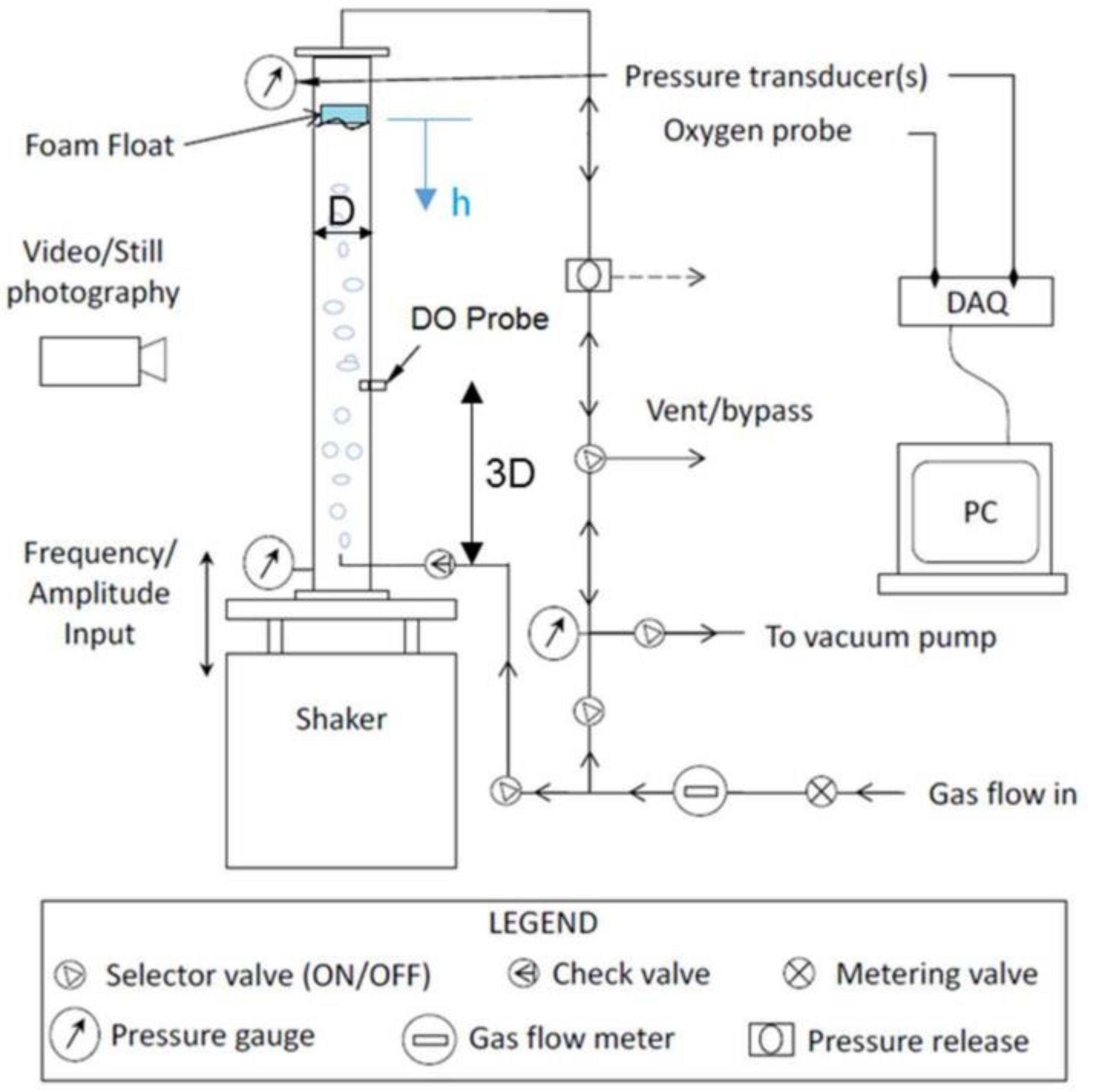
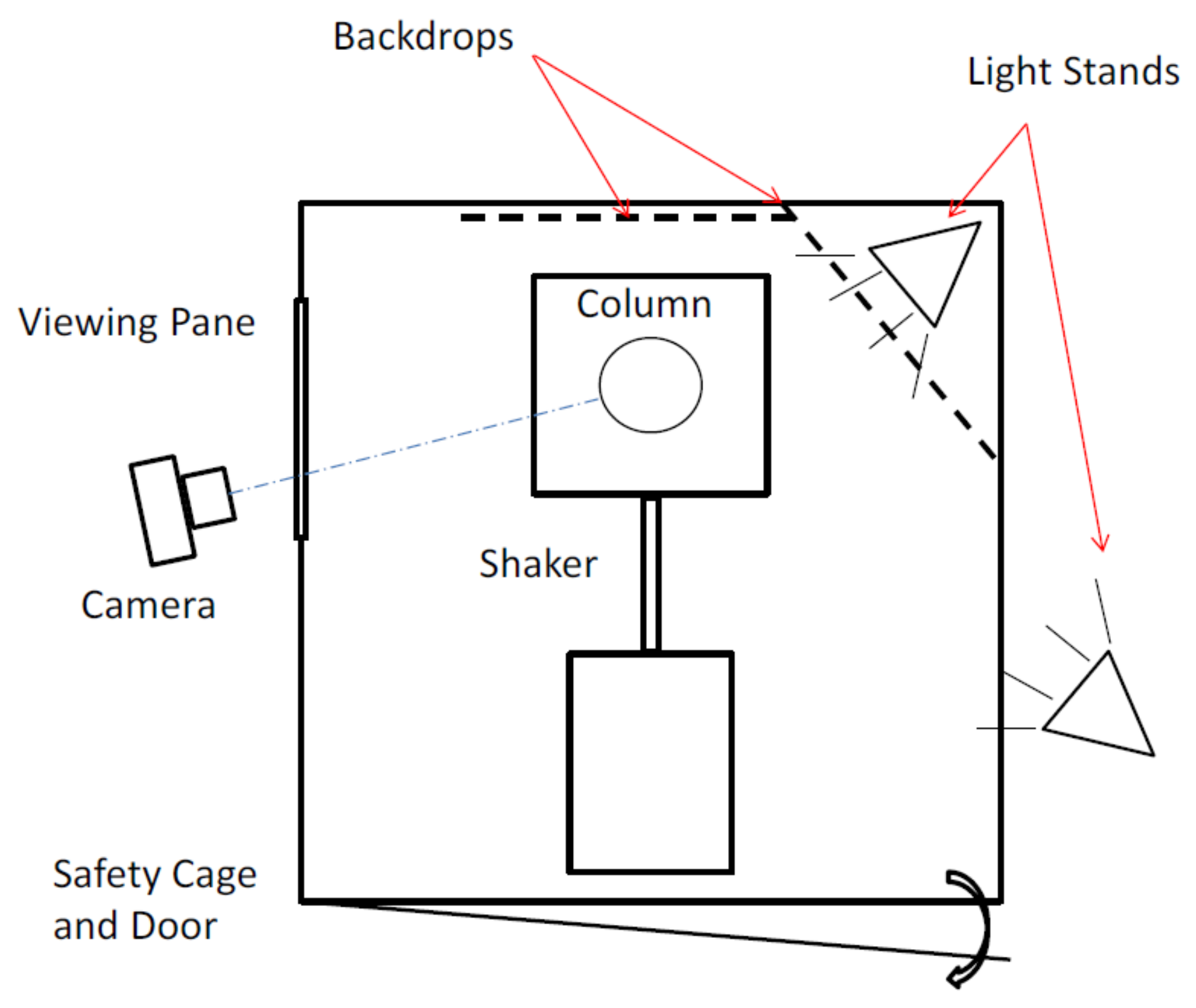
3. Experimental Methods
4. Results and Discussion
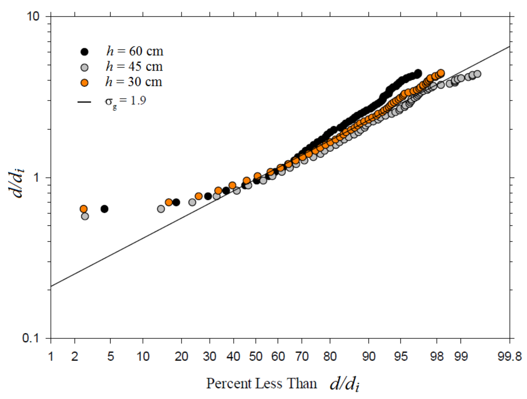
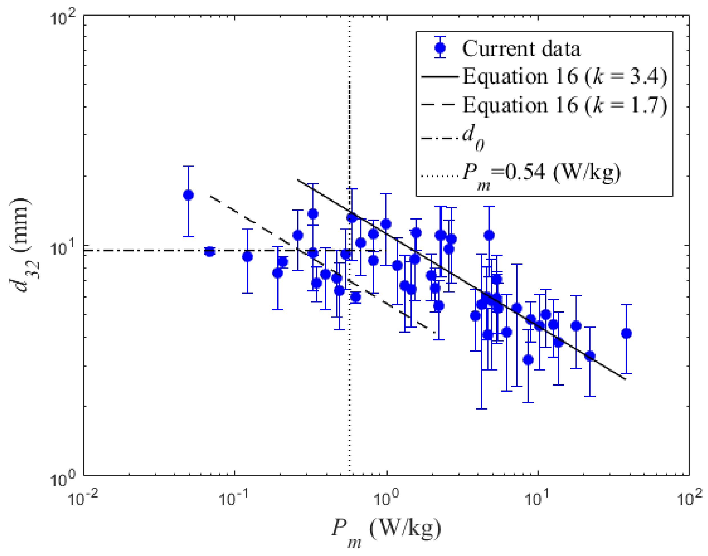
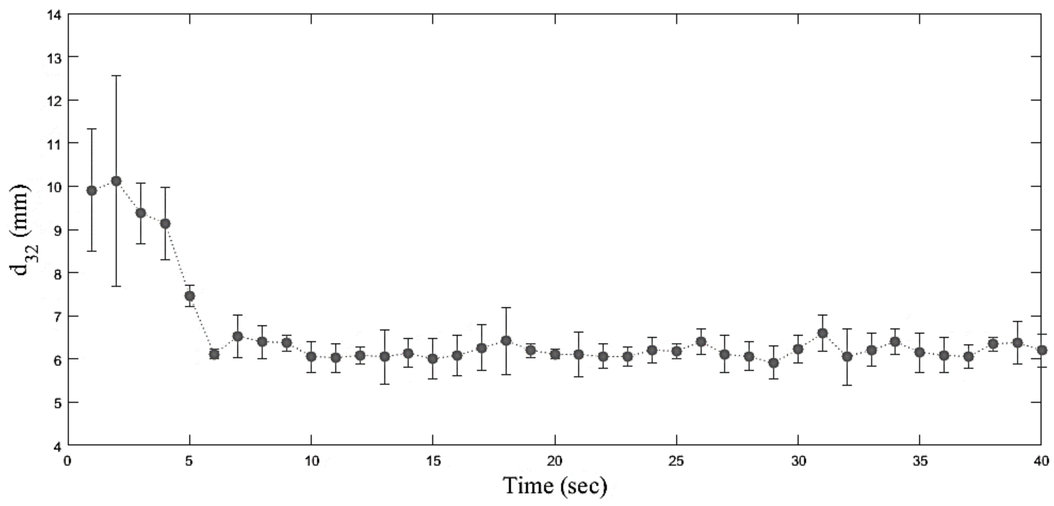
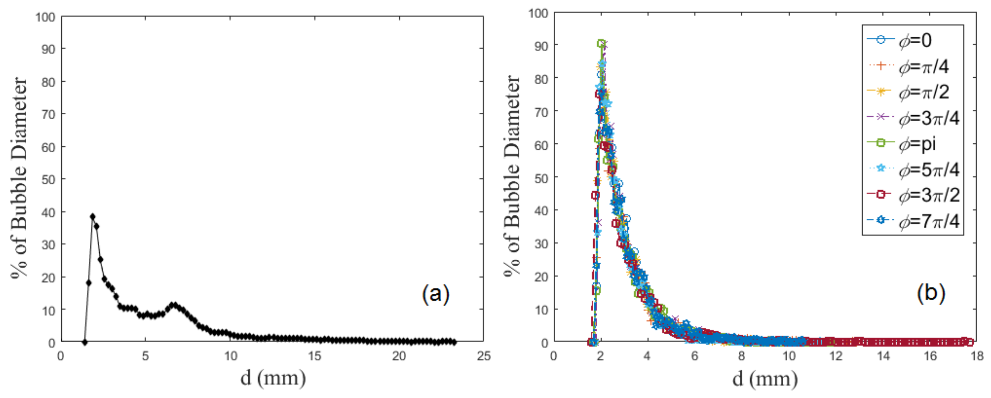
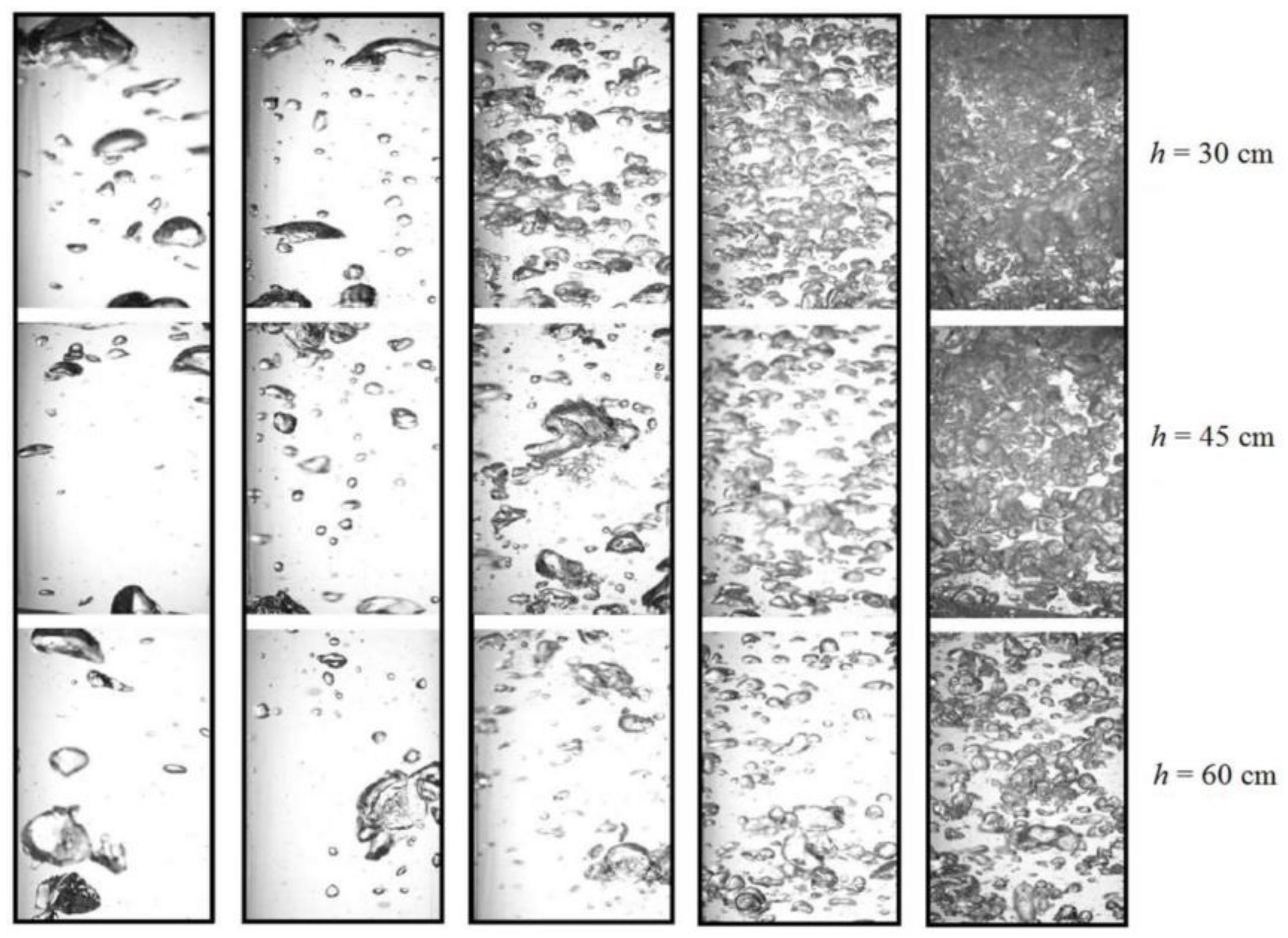
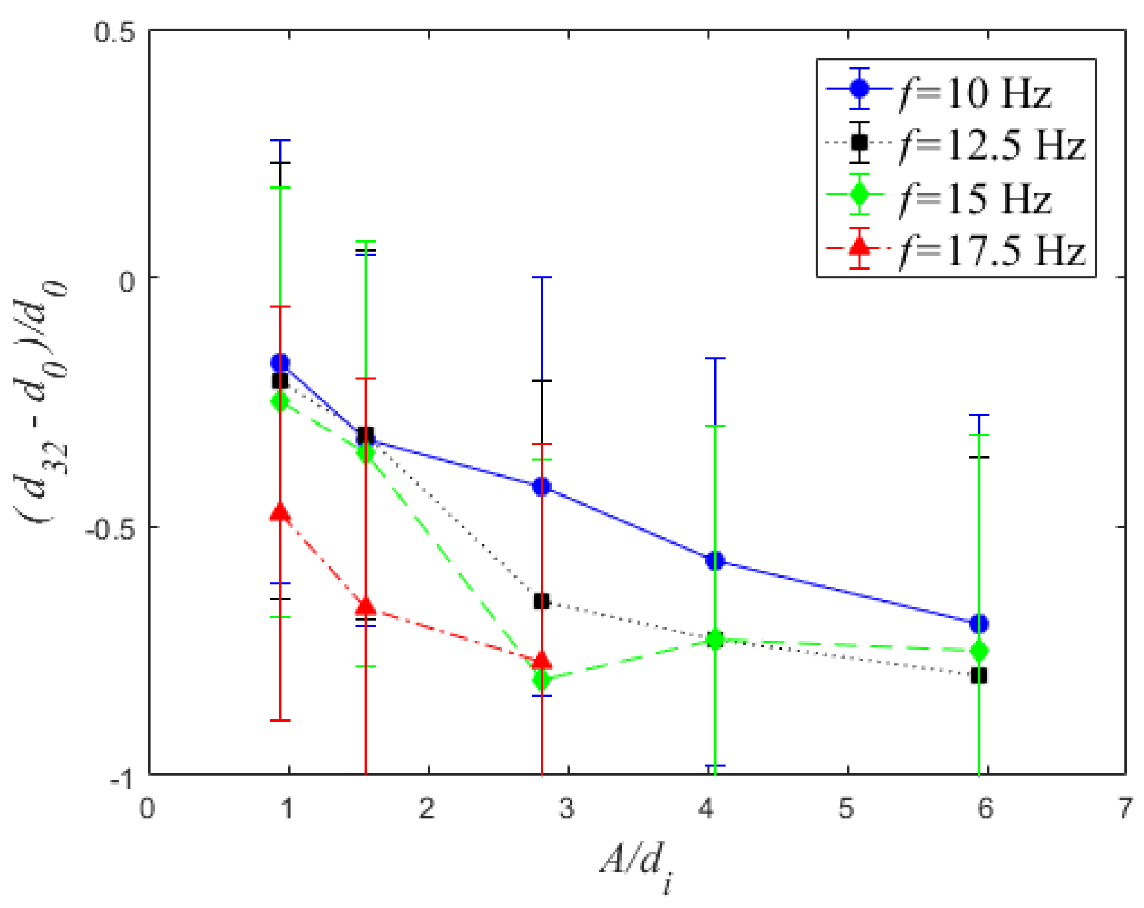
4.1. Bubble Size
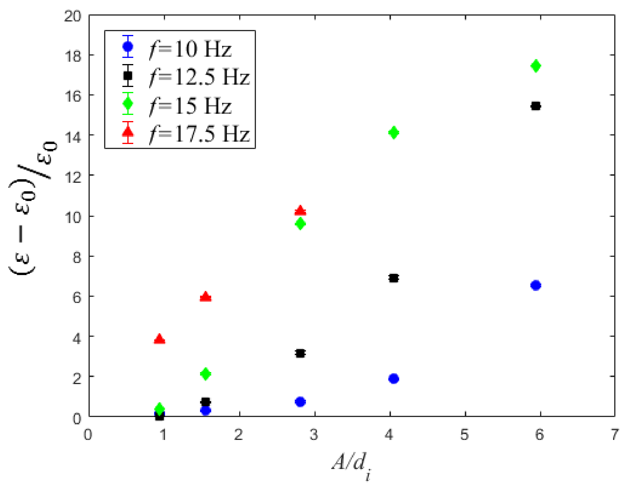
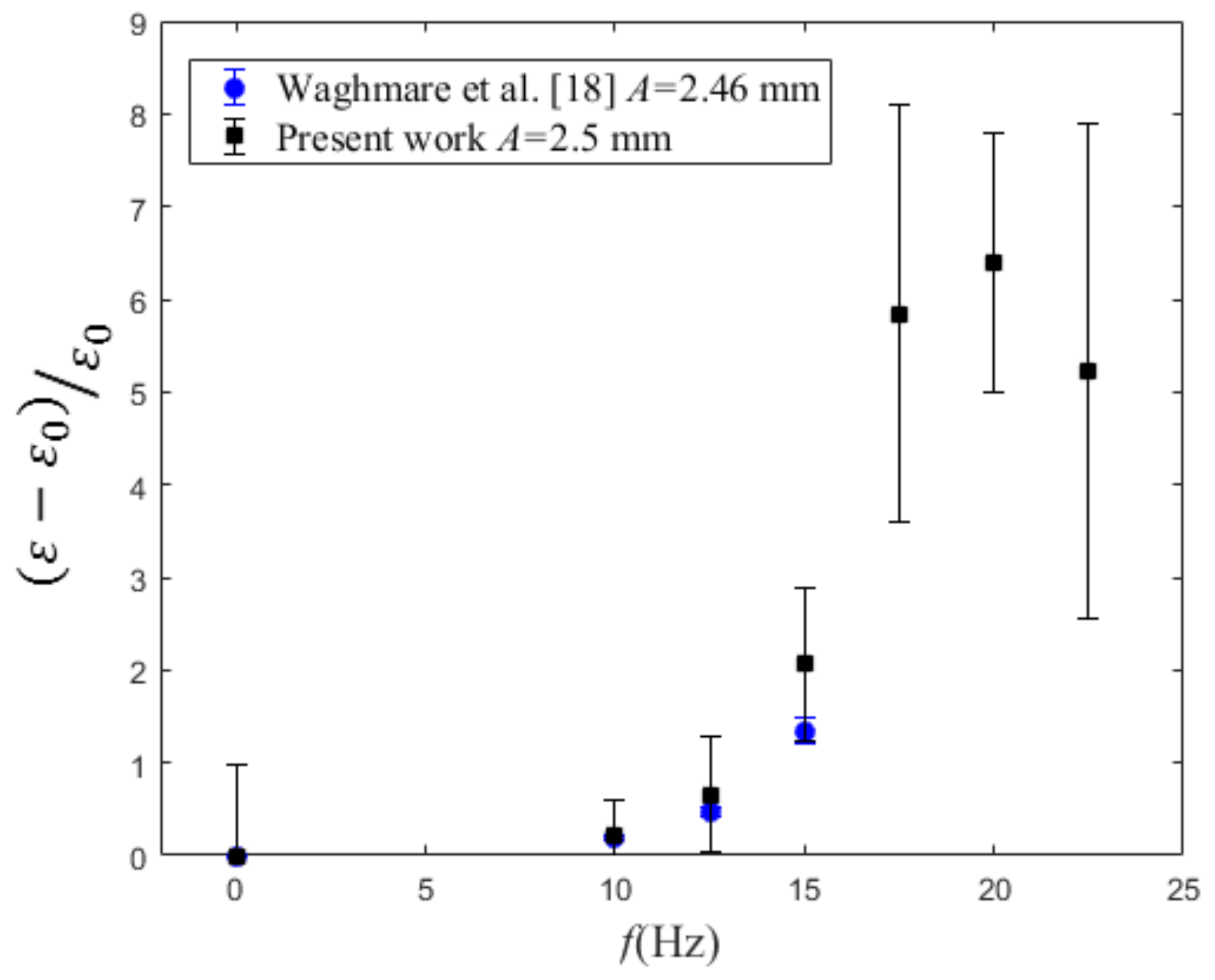
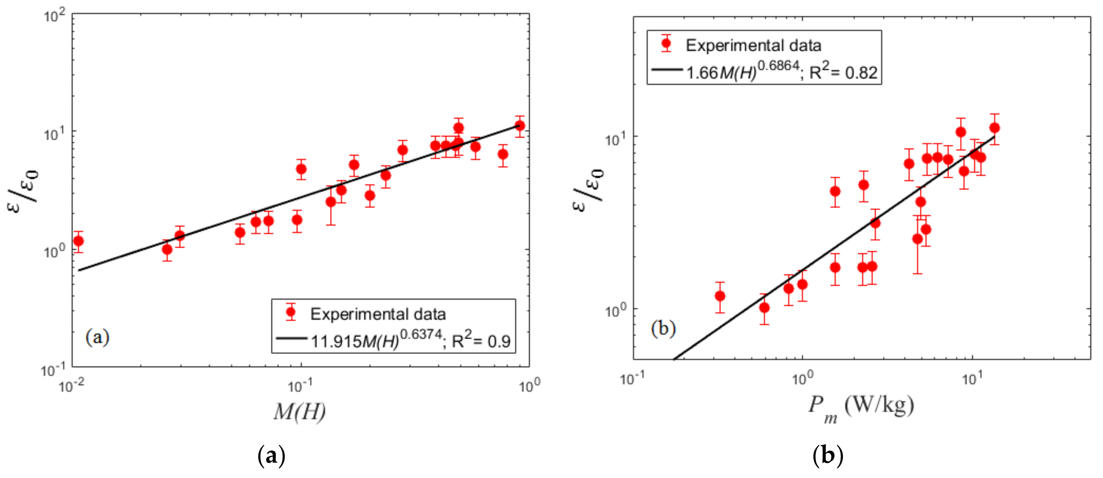
4.2. Void Fraction
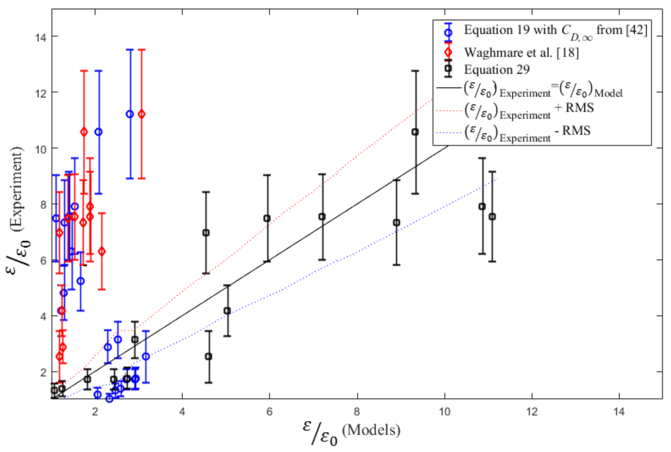
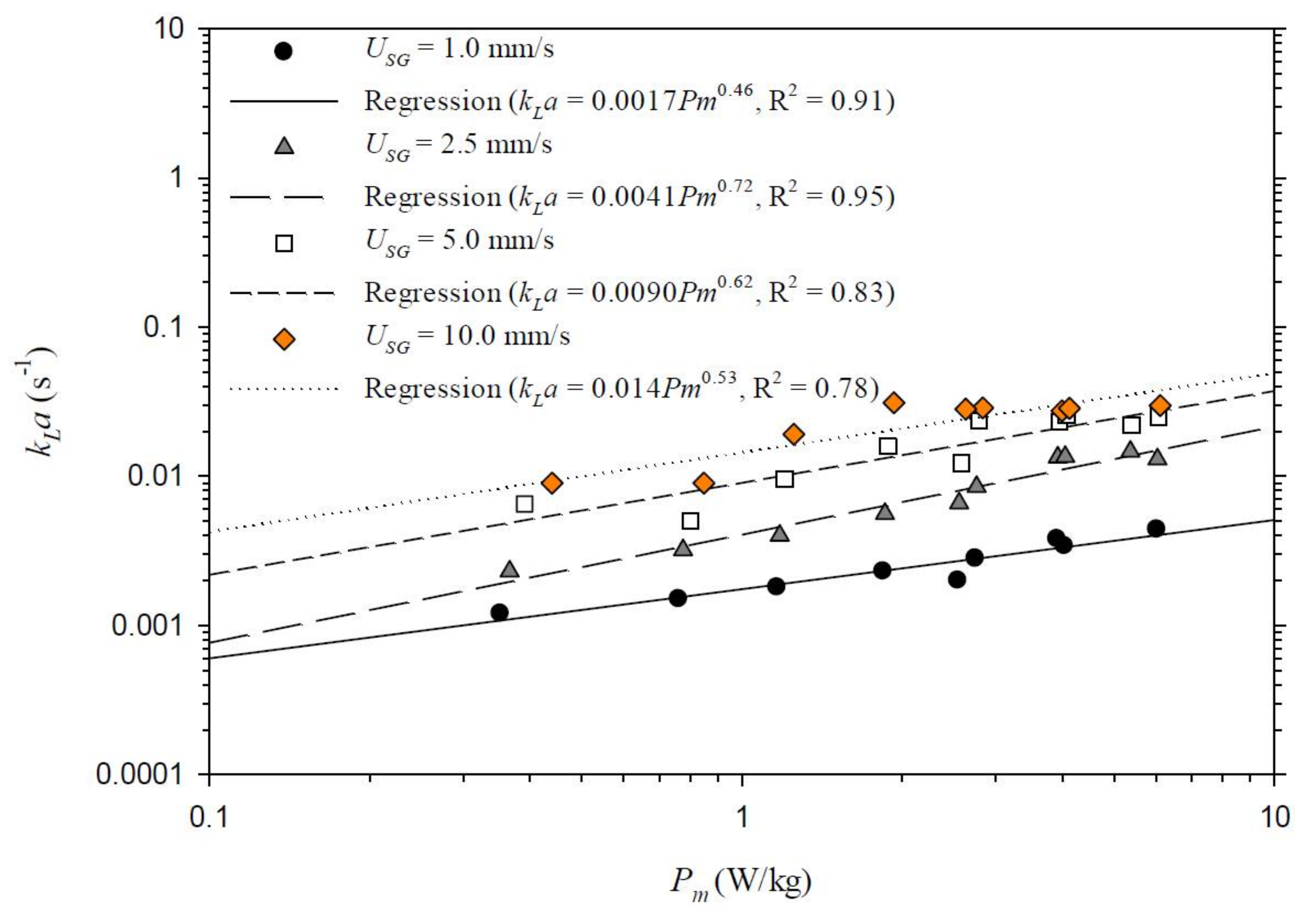
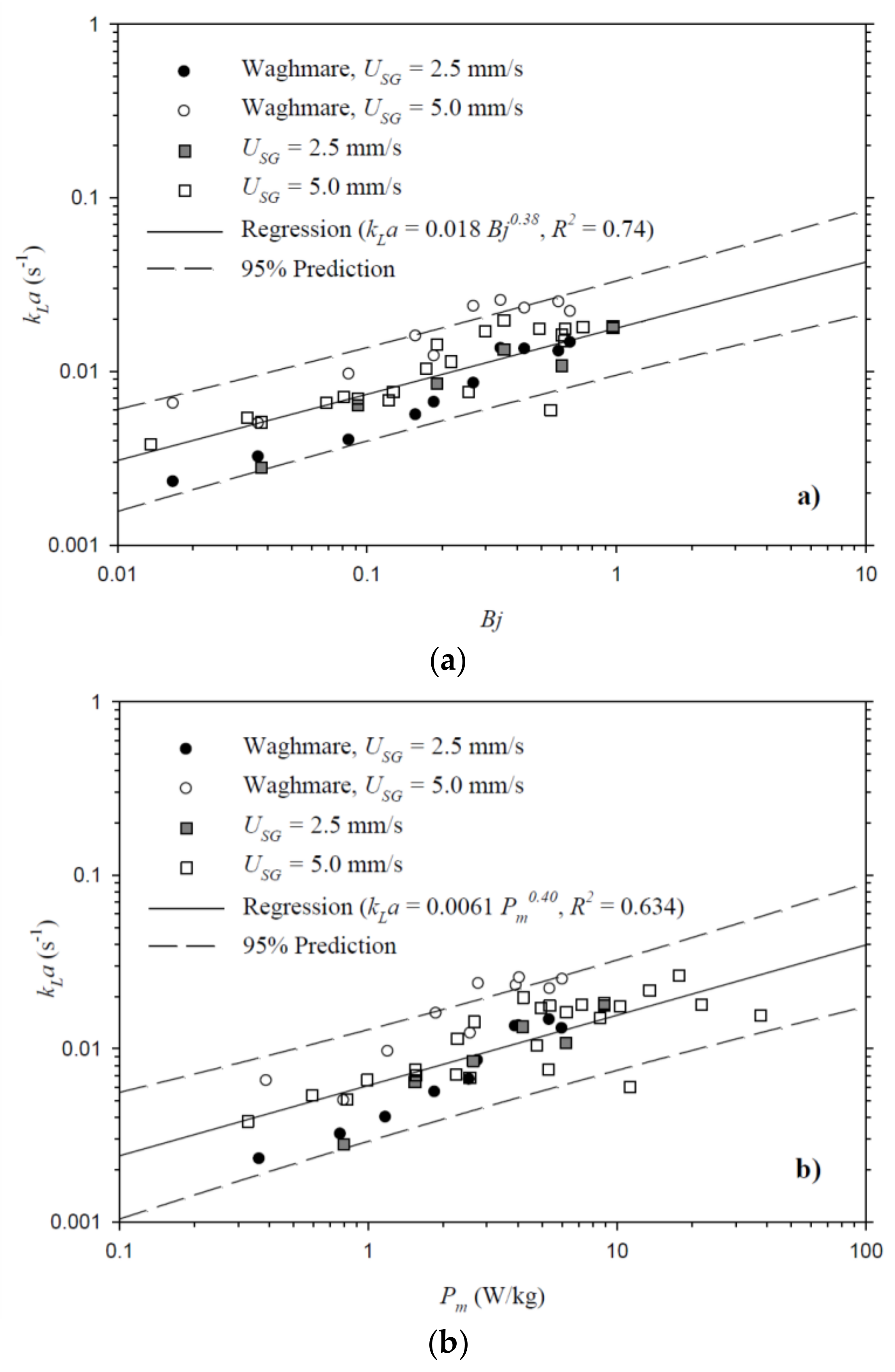
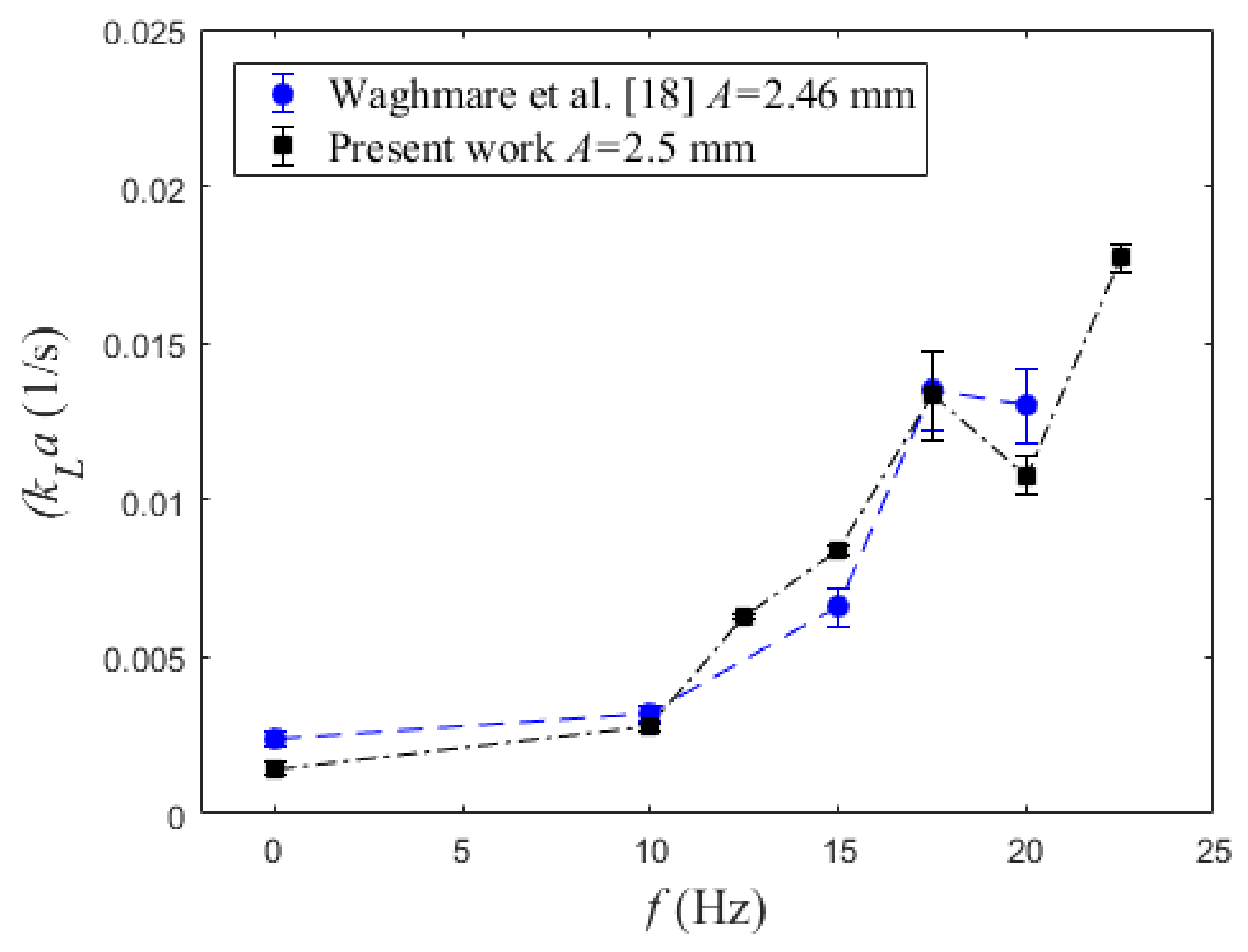
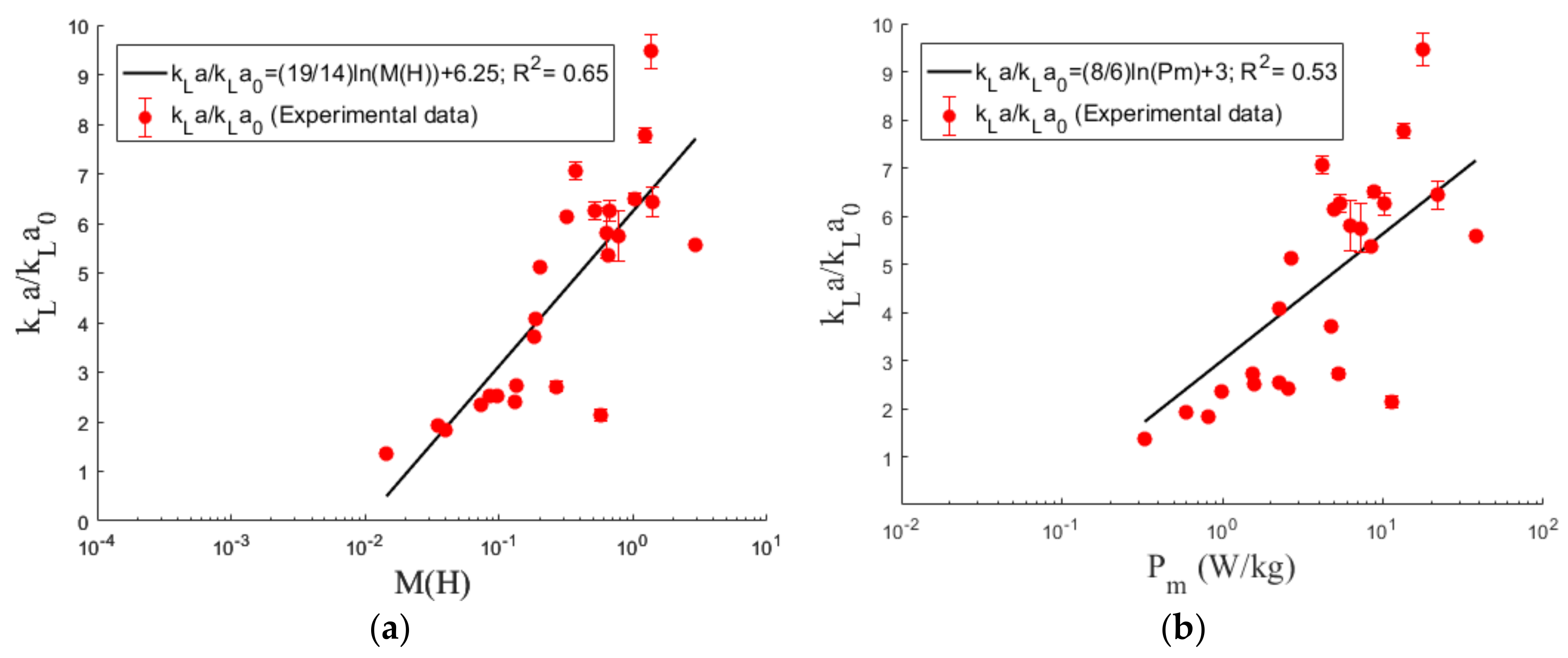
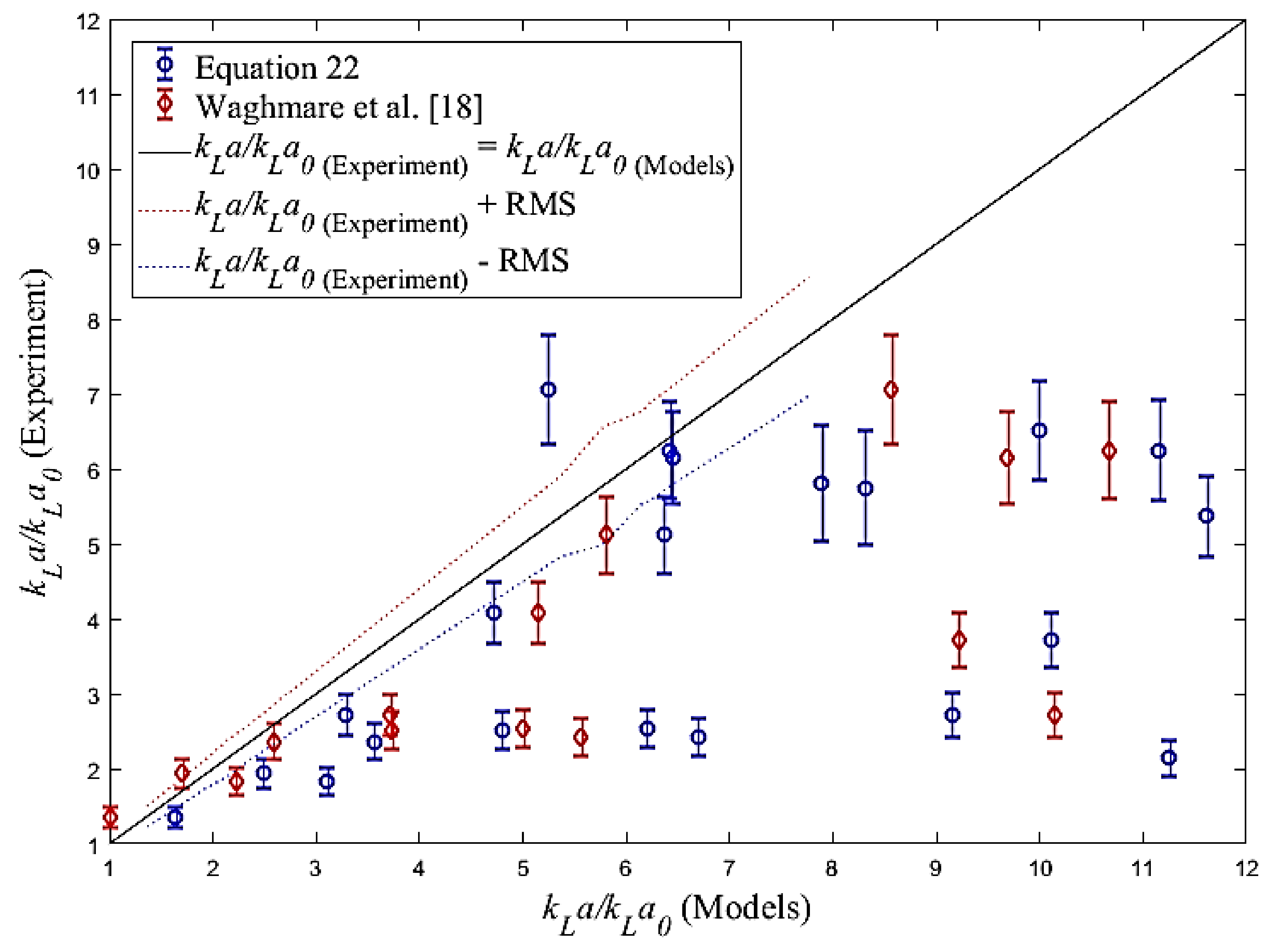
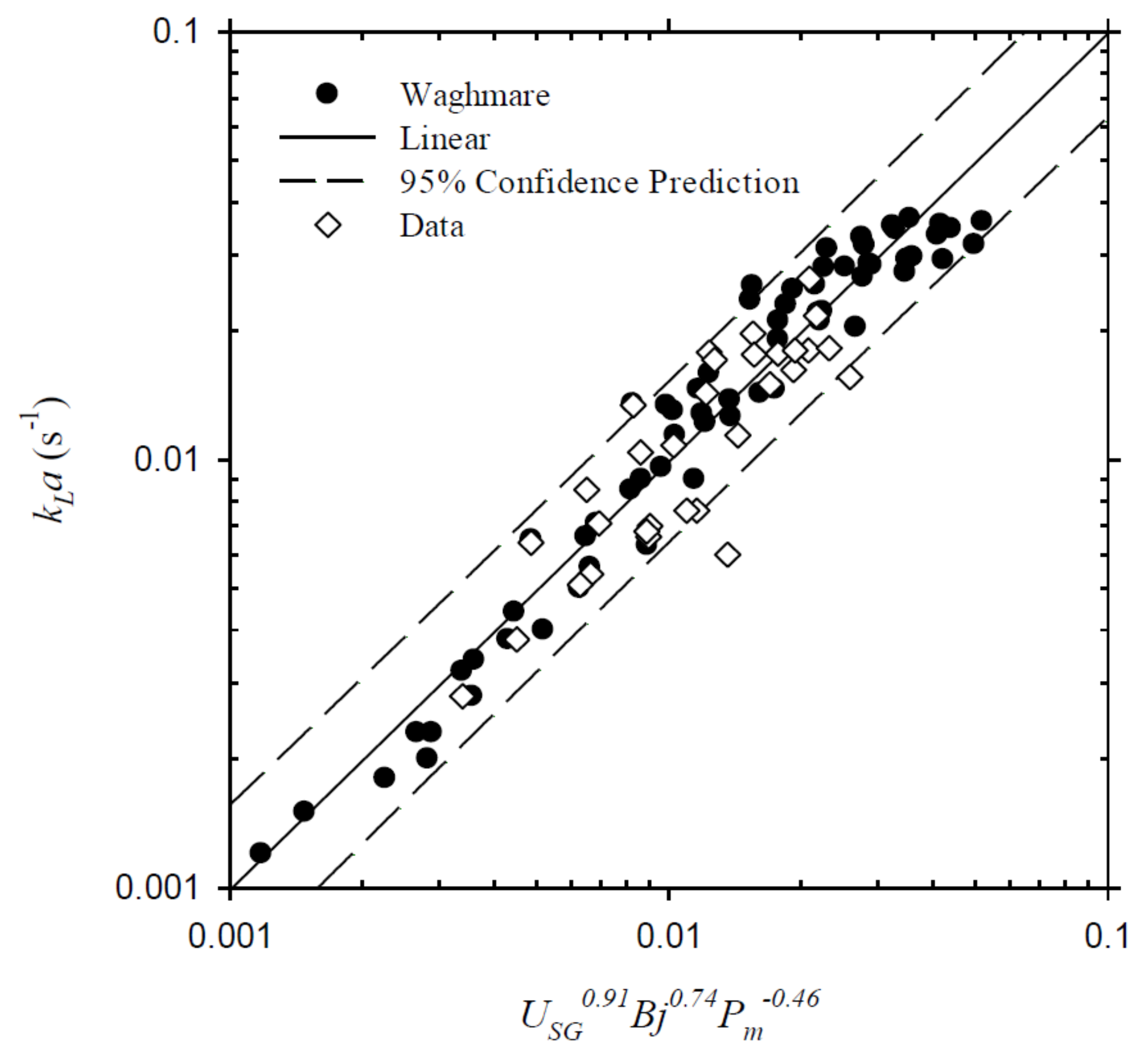
4.3. Volumetric Mass Transfer Coefficient
5. Conclusions
Acknowledgments
Author Contributions
Conflicts of Interest
Abbreviations
| Nomenclature | |
| A | Vibration Amplitude (mm) |
| ASC | Column Cross Section Area (mm2) |
| Aproj | Projected Two-Dimensional Area (mm2) |
| a | Interfacial Surface Area (mm2) |
| Bj | Bjerknes Number from Previous works [18,19,20,27] |
| C | Dissolved Gas Concentration (mg L−1) |
| C0 | Initial Dissolved Gas Concentration (mg L−1) |
| C* | Dissolved Gas Concentration at Saturation or Equilibrium (mg L−1) |
| C’ | Normalized Instantaneous Gas Concentration |
| CD | Coefficient of Drag for a Bubble Swarm |
| CD,∞ | Coefficient of Drag for a Single Isolated Bubble |
| D | Column Diameter (mm) |
| DDif | Molecular Diffusion Coefficient (mm2 s−1) |
| d | Bubble Diameter (mm) |
| deq | Area Equivalent Bubble Diameter (mm) |
| di | Injector Tube Diameter (mm) |
| d0 | Sauter Mean diameter in static column (mm) |
| d32 | Sauter Mean Diameter (mm) |
| F | Buoyancy Force (N) |
| f | Vibration Frequency (Hz) |
| fN | Bubble Resonance Frequency (Hz) |
| g | Gravitational Acceleration (m s−2) |
| HD | Dynamic Gas-Liquid Interface Height (m) |
| H | Static Liquid Height (m) |
| ∆H | Vertical Distance between Pressure Taps (m) |
| h | Liquid Height Above the Point of Interest (m) |
| K | Proportionality Coefficient in kLa Correlation |
| Kε | Proportionality Coefficient in ε Correlation |
| k | Proportionality Coefficient in Hinze Correlation |
| kL | Liquid Mass Transfer Coefficient (m/s) |
| kLa | Volumetric Mass Transfer Coefficient (s−1) |
| kLa0 | Volumetric Mass Transfer Coefficient in static column (s−1) |
| M(H) | Transient Buoyancy (Bjerknes) Number |
| Mo | Morton Number |
| m’G | Mass Flow Rate of Gas (kg s−1) |
| n | Number Count |
| PG | Gas Phase pressure at Injection Manifold (Pa) |
| Pm | Vibration Specific Power (m2 s−3) |
| Pm’(t) | Transient Vibration Specific Power (m2 s−3) |
| Pv | Liquid Vapor Pressure (Pa) |
| P0 | External or Ambient Pressure (Pa) |
| R | Transient Bubble Radius = (mm) |
| R0 | Initial Bubble Radius (in Static Column) (mm) |
| R2 | Linear Correlation Coefficient |
| P(t) | Transient Pressure from Vibration (Pa) |
| QG | Gas Volumetric flux (lit/min) |
| r | Amplitude of Bubble Oscillation (mm) |
| Re | Reynolds Number |
| Rair | Specific Ideal Gas Constant (kJ/kg K) |
| TG | Gas Phase Temperature |
| t | Time (s) |
| tc | Contact (Residence) Time (s) |
| Ub | Bubble Terminal Velocity (m/s) |
| USG | Superficial Gas Velocity (mm/s) |
| V | Bubble Volume (mm3) |
| V0 | Initial Bubble Volume (mm3) |
| We | Weber Number |
| Subscripts | |
| G | Gas |
| L | Liquid |
| Greek Symbols | |
| ε | Void Fraction |
| ε0 | Void Fraction in static column |
| κ | Gas Heat Capacity |
| μL | Liquid Dynamic Viscosity (Pa s) |
| νL | Liquid Kinematic Viscosity (m s−1) |
| ρL | Liquid Density (kg m−3) |
| ρG | Gas Density (kg m−3) |
| σ | Gas-Liquid Surface Tension (N m−1) |
| σg | Geometrical Standard Deviation |
| τ | O2 Saturation Time Scale (s) |
| Φ | Vibration Phase (Rad) |
| ω | Vibration angular velocity (Rad/s) |
References
- Harbaum, K.L.; Houghton, G. Effects of sonic vibrations on the rate of absorption of carbon dioxide in gas bubble-beds. J. Chem. Technol. Biotechnol. 1962, 12, 234–240. [Google Scholar] [CrossRef]
- Houghton, G. The behaviour of particles in a sinusoidal velocity field. Proc. R. Soc. Lond. A Math. Phys. Eng. Sci. 1963, 272, 33–43. [Google Scholar] [CrossRef]
- Jameson, G.J.; Davidson, J.F. The motion of a bubble in a vertically oscillating liquid: Theory for an inviscid liquid, and experimental results. Chem. Eng. Sci. 1966, 21, 29–34. [Google Scholar] [CrossRef]
- Jameson, G.J. The motion of a bubble in a vertically oscillating viscous liquid. Chem. Eng. Sci. 1966, 21, 35–48. [Google Scholar] [CrossRef]
- Houghton, G. Particle trajectories and terminal velocities in vertically oscillating fluids. Can. J. Chem. Eng. 1966, 44, 90–95. [Google Scholar] [CrossRef]
- Rubin, E. Behavior of gas bubbles in vertically vibrating liquid columns. Can. J. Chem. Eng. 1968, 46, 145–149. [Google Scholar] [CrossRef]
- Foster, J.M.; Botts, J.A.; Barbin, A.R.; Vachon, R.I. Bubble trajectories and equilibrium levels in vibrated liquid columns. J. Basic Eng. 1986, 90, 125–132. [Google Scholar] [CrossRef]
- Marmur, A.; Rubin, E. Viscous effect on stagnation depth of bubbles in a vertically oscillating liquid column. Can. J. Chem. Eng. 1976, 54, 509–514. [Google Scholar] [CrossRef]
- Tojo, K.; Nishimura, K.; Iwanaka, H.; Miyanami, K. Particle Movement in a Vertically Oscillating Liquid. Bull. Univ. Osaka Prefect. Ser. A Eng. Nat. Sci. 1981, 30, 41–53. [Google Scholar]
- Baird, M.H.I.; Garstang, J.H. Gas absorption in a pulsed bubble column. Chem. Eng. Sci. 1972, 27, 823–833. [Google Scholar] [CrossRef]
- Bretsznajder, S.; Jaszczak, M.; Pasiuk, W. Increasing the rate of certain industrial chemical processes by the use of vibration. Ind. Chem. Eng. 1963, 3, 496–502. [Google Scholar]
- Krishna, R.; Ellenberger, J.; Urseanu, M.I.; Keil, F.J. Utilisation of bubble resonance phenomena to improve ga-liquid contact. Naturwissenschaften 2000, 87, 455–459. [Google Scholar] [CrossRef] [PubMed]
- Krishna, R.; Ellenberger, J. Improving ga-liquid contacting in bubble columns by vibration excitement. International journal of multiphase flow. Int. J. Multiph. Flow 2002, 28, 1223–1234. [Google Scholar] [CrossRef]
- Ellenberger, J.; Krishna, R. Shaken, not stirred, bubble column reactors: Enhancement of mass transfer by vibration excitement. Chem. Eng. Sci. 2003, 58, 705–710. [Google Scholar] [CrossRef]
- Ellenberger, J.; Van Baten, J.M.; Krishna, R. Exploiting the Bjerknes force in bubble column reactors. Chem. Eng. Sci. 2005, 60, 5962–5970. [Google Scholar] [CrossRef]
- Knopf, F.C.; Ma, J.; Rice, R.G.; Nikitopoulos, D. Pulsing to improve bubble column performance: I. Low gas rates. AIChE J. 2006, 52, 1103–1115. [Google Scholar] [CrossRef]
- Knopf, F.C.; Waghmare, Y.; Ma, J.; Rice, R.G. Pulsing to improve bubble column performance: II. Jetting gas rates. AIChE J. 2006, 52, 1116–1126. [Google Scholar] [CrossRef]
- Waghmare, Y.G.; Knopf, F.C.; Rice, R.G. The Bjerknes effect: Explaining pulsed-flow behavior in bubble columns. AIChE J. 2007, 53, 1678–1686. [Google Scholar] [CrossRef]
- Waghmare, Y.G.; Rice, R.G.; Knopf, F.C. Mass transfer in a viscous bubble column with forced oscillations. Ind. Eng. Chem. Res. 2008, 47, 5386–5394. [Google Scholar] [CrossRef]
- Waghmare, Y.G.; Dorao, C.A.; Jakobsen, H.A.; Knopf, F.C.; Rice, R.G. Bubble size distribution for a bubble column reactor undergoing forced oscillations. Ind. Eng. Chem. Res. 2009, 48, 1786–1796. [Google Scholar] [CrossRef]
- Budzyński, P.; Dziubiński, M. Intensification of bubble column performance by introduction pulsation of liquid. Chem. Eng. Proc. Process Intensif. 2014, 78, 44–57. [Google Scholar] [CrossRef]
- Budzyński, P.; Gwiazda, A.; Dziubiński, M. Intensification of mass transfer in a pulsed bubble column. Chem. Eng. Proc. Process Intensif. 2017, 112, 18–30. [Google Scholar] [CrossRef]
- Gaddis, E.S. Mass transfer in ga-liquid contactors. Chem. Eng. Proc. Process Intensif. 1999, 38, 503–510. [Google Scholar] [CrossRef]
- Mohagheghian, S.; Elbing, B.R. Characterization of Bubble Size Distributions within a Bubble Column. Fluids 2018, 3, 13. [Google Scholar] [CrossRef]
- Hur, Y.G.; Yang, J.H.; Jung, H.; Park, S.B. Origin of regime transition to turbulent flow in bubble column: Orifice- and column-induced transitions. Int. J. Multiph. Flow 2013, 50, 89–97. [Google Scholar] [CrossRef]
- Oliveira, M.S.N.; Ni, X. Gas hold-up and bubble diameters in a gassed oscillatory baffled column. Chem. Eng. Sci. 2001, 56, 6143–6148. [Google Scholar] [CrossRef]
- Still, A.L.; Ghajar, A.J.; O’Hern, T.J. Effect of amplitude on mass transport, void fraction and bubble size in a vertically vibrating liquid-gas bubble column reactor. In Proceedings of the ASME 2013 Fluids Engineering Division Summer Meeting, Incline Village, NV, USA, 7–11 July 2013; p. V01CT17A004. [Google Scholar]
- Elbing, B.R.; Still, A.L.; Ghajar, A.J. Review of bubble column reactors with vibration. Ind. Eng. Chem. Res. 2016, 55, 385–403. [Google Scholar] [CrossRef]
- Besagni, G.; Inzoli, F.; Ziegenhein, T. Two-Phase Bubble Columns: A Comprehensive Review. ChemEngineering 2018, 2, 13. [Google Scholar] [CrossRef]
- Simonnet, M.; Gentric, C.; Olmos, E.; Midoux, N. Experimental determination of the drag coefficient in a swarm of bubbles. Chem. Eng. Sci. 2007, 62, 858–866. [Google Scholar] [CrossRef]
- Hinze, J.O. Fundamentals of the hydrodynamic mechanism of splitting in dispersion processes. AIChE J. 1955, 1, 289–295. [Google Scholar] [CrossRef]
- Lewis, D.; Davidson, J.F. Bubble splitting in shear flow. Trans. Inst. Chem. Eng. 1982, 60, 283–291. [Google Scholar]
- Wilkinson, P.M.; Spek, A.P.; van Dierendonck, L.L. Design parameters estimation for scale-up of high-pressure bubble columns. AIChE J. 1992, 38, 544–554. [Google Scholar] [CrossRef]
- Gaddis, E.S.; Vogelpohl, A. Bubble formation in quiescent liquids under constant flow conditions. Chem. Eng. Sci. 1986, 41, 97–105. [Google Scholar] [CrossRef]
- Besagni, G.; Inzoli, F. Novel gas holdup and regime transition correlation for two-phase bubble columns. In Journal of Physics: Conference Series; IOP Publishing: Bristol, UK, 2017. [Google Scholar]
- Besagni, G.; Di Pasquali, A.; Gallazzini, L.; Gottardi, E.; Colombo, L.P.M.; Inzoli, F. The effect of aspect ratio in counter-current gas-liquid bubble columns: Experimental results and gas holdup correlations. Int. J. Multiph. Flow 2017, 94, 53–78. [Google Scholar] [CrossRef]
- Clark, N.N.; Atkinson, C.M.; Flemmer, R.L.C. Turbulent circulation in bubble columns. AIChE J. 1987, 33, 515–518. [Google Scholar] [CrossRef]
- Abràmoff, M.D.; Magalhães, P.J.; Ram, S.J. Image processing with ImageJ. Biophotonics Int. 2004, 11, 36–42. [Google Scholar]
- Schneider, C.A.; Rasband, W.S.; Eliceiri, K.W. NIH Image to ImageJ: 25 years of image analysis. Nat. Methods 2012, 9, 671–675. [Google Scholar] [CrossRef] [PubMed]
- Rasband, W.S. ImageJ. U.S. National Institutes of Health: Bethesda, MD, USA, 1997–2016. Available online: http://imagej.nih.gov/ij (accessed on 16 April 2013).
- Besagni, G.; Inzoli, F.; Ziegenhein, T.; Lucas, D. Computational Fluid-Dynamic modeling of the pseudo-homogeneous flow regime in large-scale bubble columns. Chem. Eng. Sci. 2017, 160, 144–160. [Google Scholar] [CrossRef]
- Guédon, G.R.; Besagni, G.; Inzoli, F. Prediction of ga-liquid flow in an annular gap bubble column using a bi-dispersed Eulerian model. Chem. Eng. Sci. 2017, 161, 138–150. [Google Scholar] [CrossRef]
- Hedrick, T.L. Software techniques for two-and three-dimensional kinematic measurements of biological and biomimetic systems. Bioinspiration Biomim. 2008, 3, 034001. [Google Scholar] [CrossRef] [PubMed]
- Xue, J.; Al-Dahhan, M.; Dudukovic, M.P.; Mudde, R.F. Bubble velocity, size, and interfacial area measurements in a bubble column by four-point optical probe. AIChE J. 2008, 54, 350–363. [Google Scholar] [CrossRef]
- Xue, J.; Al-Dahhan, M.; Dudukovic, M.P.; Mudde, R.F. Four-point optical probe for measurement of bubble dynamics: Validation of the technique. Flow Meas. Inst. 2008, 19, 293–300. [Google Scholar] [CrossRef]
- Miyauchi, T.; Oya, H. Longitudinal dispersion in pulsed perforated-plate columns. AIChE J. 1965, 11, 395–402. [Google Scholar] [CrossRef]
- Bhaga, D.; Weber, M.E. Bubbles in viscous liquids: Shapes, wakes and velocities. J. Fluid Mech. 1981, 105, 61–85. [Google Scholar] [CrossRef]
- Brennen, C.E. Fundamental of Multiphase Flow, 1st ed.; Cambridge University Press: New York, NY, USA, 2005; pp. 60–66. ISBN 0521139988. [Google Scholar]
- Majumder, S.K. Hydrodynamics and Transport Processes of Inverse Bubbly Flow; Elsevier: New York, NY, USA, 2016. [Google Scholar]
- Hashimoto, H.; Sudo, S. Surface disintegration and bubble formation in vertically vibrated liquid column. AIAA J. 1980, 18, 442–449. [Google Scholar]
- Hashimoto, H.; Sudo, S. Dynamic behavior of liquid free surface in a cylindrical container subjected to vertical vibration. Bull. JSME 1984, 27, 923–930. [Google Scholar] [CrossRef]


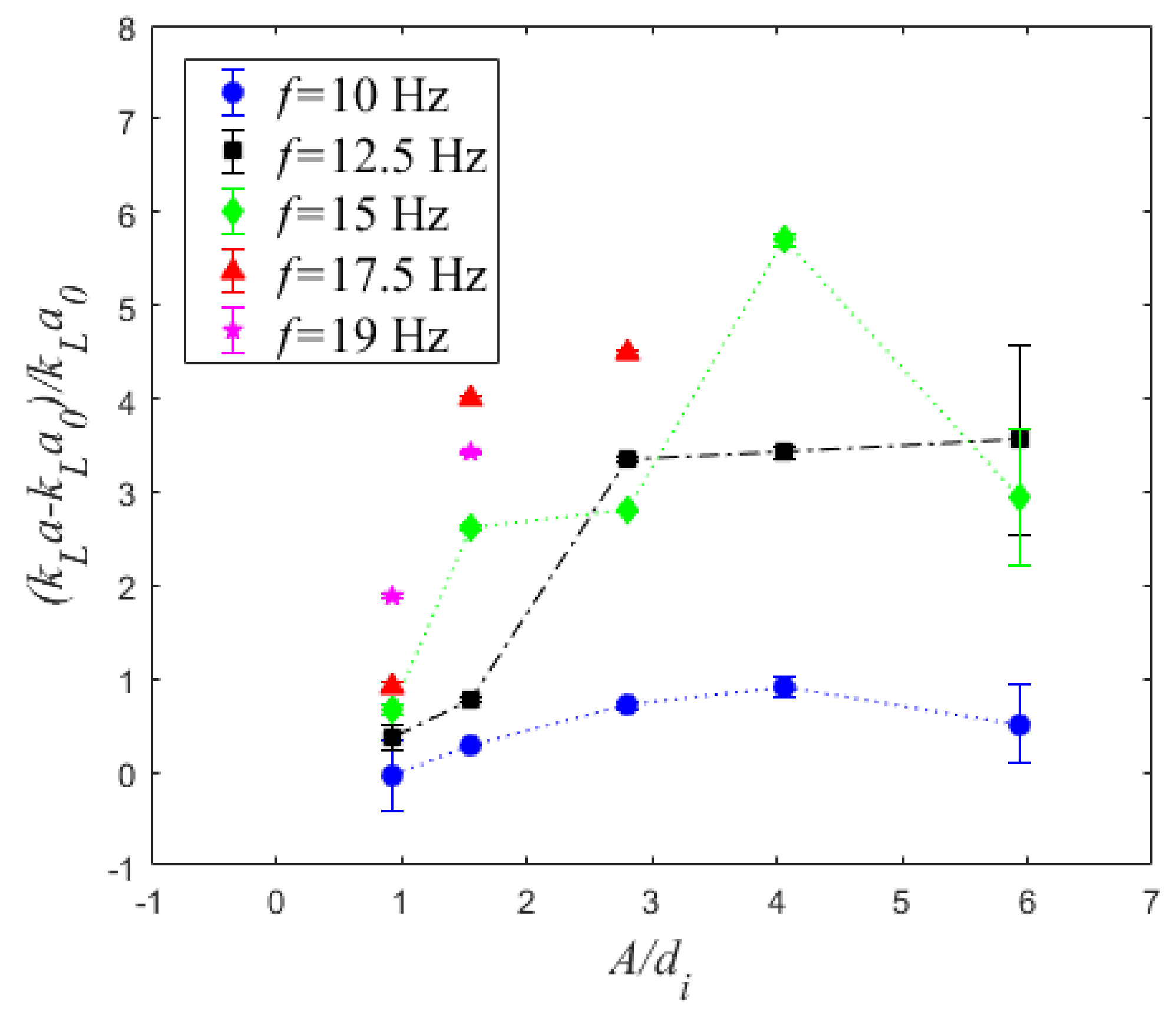
| f (Hz) | A = 1.5 mm | A = 2.5 mm | A = 4.5 mm | A = 6.5 mm | A = 9.5 mm |
|---|---|---|---|---|---|
| 7.5 | - | - | - | 2.7 | 4 |
| 10 | 1.5 | 2 | 2.6 | 2.9 | 2.3 |
| 12.5 | 2.1 | 2.7 | 6.6 | 6.8 | 6.9 |
| 15 | 2.5 | 5.5 | 5.8 | 10.2 | 6 |
| 17.5 | 2.9 | 7.6 | 8.3 | - | - |
| 20 | 4.4 | 6.2 | - | - | - |
| 22.5 | - | 7 | - | - | - |
© 2018 by the authors. Licensee MDPI, Basel, Switzerland. This article is an open access article distributed under the terms and conditions of the Creative Commons Attribution (CC BY) license (http://creativecommons.org/licenses/by/4.0/).
Share and Cite
Mohagheghian, S.; Still, A.L.; Elbing, B.R.; Ghajar, A.J. Study of Bubble Size, Void Fraction, and Mass Transport in a Bubble Column under High Amplitude Vibration. ChemEngineering 2018, 2, 16. https://doi.org/10.3390/chemengineering2020016
Mohagheghian S, Still AL, Elbing BR, Ghajar AJ. Study of Bubble Size, Void Fraction, and Mass Transport in a Bubble Column under High Amplitude Vibration. ChemEngineering. 2018; 2(2):16. https://doi.org/10.3390/chemengineering2020016
Chicago/Turabian StyleMohagheghian, Shahrouz, Adam L. Still, Brian R. Elbing, and Afshin J. Ghajar. 2018. "Study of Bubble Size, Void Fraction, and Mass Transport in a Bubble Column under High Amplitude Vibration" ChemEngineering 2, no. 2: 16. https://doi.org/10.3390/chemengineering2020016
APA StyleMohagheghian, S., Still, A. L., Elbing, B. R., & Ghajar, A. J. (2018). Study of Bubble Size, Void Fraction, and Mass Transport in a Bubble Column under High Amplitude Vibration. ChemEngineering, 2(2), 16. https://doi.org/10.3390/chemengineering2020016