Quantitative Characterization of Arnicae flos by RP-HPLC-UV and NIR Spectroscopy


Abstract
1. Introduction
2. Materials and Methods
2.1. Sample Material
2.2. HPLC-Analysis
- For the phenolic compounds—Hypersil ODS C18, 5 μm, 250 × 4.6 mm I.D. (Shandon, Runcom, England), with precolumn 30 × 4.6 mm (Interchim, Montluço France) with the same adsorbent.
- For the sesquiterpene lactones—Luna 5 μm C18 100 A, 150 × 4.6 mm (Phenomenex, Torrance, CA, USA), with precolumn 30 × 4.6 mm (Interchim, Montluçon, France) with the same adsorbent.
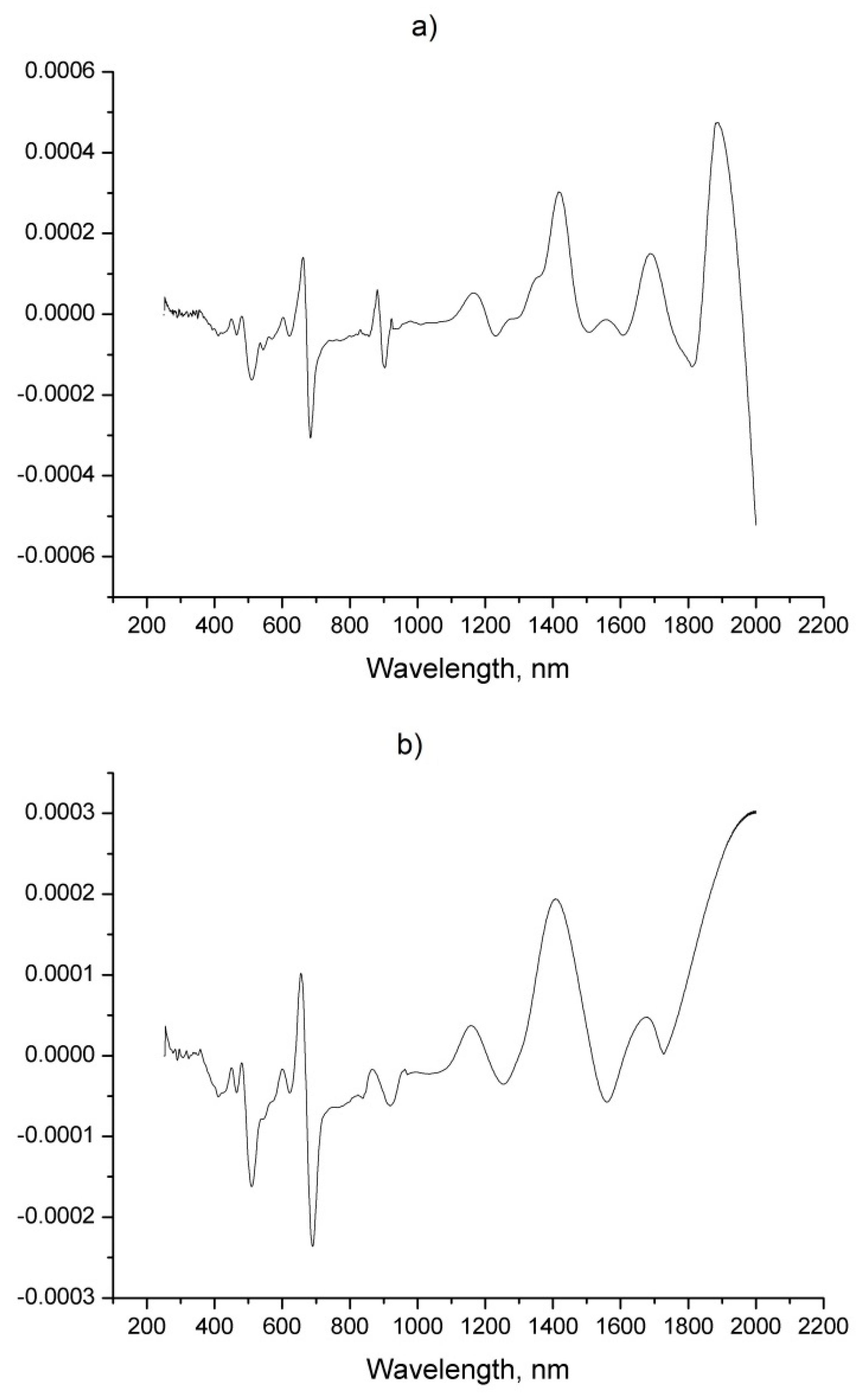
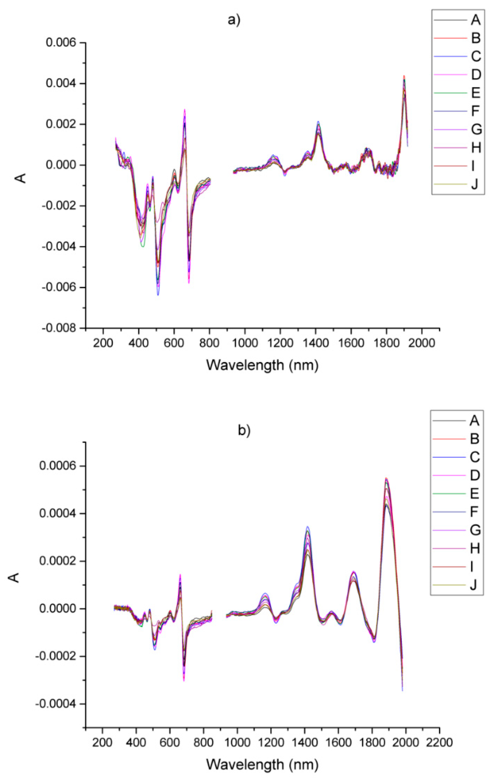
2.3. Spectral Measurements
- 270–850; 907–2000 nm for non-derivate spectra,
- 270–850; 935–1920 nm for spectra treated with GS,
- 270–850; 935–1980 nm for spectra treated with SBSF,
2.4. Data Processing
- choosing the lowest value of RMSECV or
- selecting the lowest number of PCs by which the largest percentage of variation can be described
3. Results and Discussion
4. Conclusions
Author Contributions
Funding
Acknowledgments
Conflicts of Interest
References
- Merfort, I. Arnika: Neue Erkenntnisse zum Wirkungsmechanismus einer traditionellen Heilpflanze. Complement. Med. Res. 2003, 10, 45–48. [Google Scholar] [CrossRef]
- Elena, G.M. Biodiversity and Protection of the Medicinal and Aromatic Plants in Bulgaria; Association for Medicinal and Aromatic Plants of Southeast European Countries (AMAPSEEC): Belgrade, Serbia, 2006. [Google Scholar]
- Alcalà, M.; Blanco, M.; Moyano, D.; Broad, N.W.; O’Brien, N.; Friedrich, D.; Pfeifer, F.; Siesler, H.W. Qualitative and Quantitative Pharmaceutical Analysis with a Novel Hand-Held Miniature near Infrared Spectrometer. J. Infrared Spectrosc. 2013, 21, 445–457. [Google Scholar] [CrossRef]
- Knuesel, O.; Weber, M.; Suter, A. Arnica montana gel in osteoarthritis of the knee: An open, multicenter clinical trial. Adv. Ther. 2002, 19, 209–218. [Google Scholar] [CrossRef]
- Ganzera, M.; Egger, C.; Zidorn, C.; Stuppner, H. Quantitative analysis of flavonoids and phenolic acids in Arnica montana L. by micellar electrokinetic capillary chromatography. Anal. Chim. Acta 2008, 614, 196–200. [Google Scholar] [CrossRef]
- Staneva, J.; Denkova, P.; Todorova, M.; Evstatieva, L. Quantitative analysis of sesquiterpene lactones in extract of Arnica montana L. by 1H NMR spectroscopy. J. Pharm. Biomed. Anal. 2011, 54, 94–99. [Google Scholar] [CrossRef] [PubMed]
- Stefanache, C.; Bujor, O.; Necula, R.; Grigoras, V.; Mardari, C.; Birsan, C.; Danila, D. Sesquiterpene lactones and phenolic compounds content in Arnica montana flowers and leaves samples harvested from wild sites in North-East Romania. Planta Med. 2016, 81, S1–S381. [Google Scholar] [CrossRef]
- Albert, A.; Sareedenchai, V.; Heller, W.; Seidlitz, H.K.; Zidorn, C. Temperature is the key to altitudinal variation of phenolics in Arnica montana L. cv. ARBO. Oecologia 2009, 160, 1–8. [Google Scholar] [CrossRef] [PubMed]
- Lange, D. Europe’s Medicinal and Aromatic Plants: Their Use, Trade and Conservation; Traffic International: Cambridge, UK, 1998. [Google Scholar]
- Albert, H.; Biertümpfel, A.; Blaschek, W.; Blüthner, W.D.; Böhme, M.; Bomme, U.; Brunner, P.; Carlen, C.; Adam, L. Handbuch des Arznei-und Gewürzpflanzenbaus, Band 4; Verein für Arznei- und Gewürzpflanzen: Bernburg, Germany, 2012; pp. 54–86. [Google Scholar]
- Savitzky, A.; Golay, M.J.E. Smoothing and Differentiation of Data by Simplified Least Squares Procedures. Anal. Chem. 1964, 36, 1627–1639. [Google Scholar] [CrossRef]
- Steinier, J.; Termonia, Y.; Deltour, J. Smoothing and differentiation of data by simplified least square procedure. Anal. Chem. 1972, 44, 1906–1909. [Google Scholar] [CrossRef] [PubMed]
- Antonov, L. An alternative for the calculation of derivative spectra in the near-infrared spectroscopy. J. Infrared Spectrosc. 2017, 25, 145–148. [Google Scholar] [CrossRef]
- Jaiswal, R.; Kuhnert, N. Identification and Characterization of Two New Derivatives of Chlorogenic Acids in Arnica (Arnica montana L.) Flowers by High-Performance Liquid Chromatography/Tandem Mass Spectrometry. J. Agric. Food Chem. 2011, 59, 4033–4039. [Google Scholar] [CrossRef] [PubMed]
- Merfort, I.; Pietta, P.G.; Mauri, P.L.; Zini, L.; Catalano, G.; Willuhn, G. Separation of Sesquiterpene Lactones from Arnicae Flos DAB 10 by Micellar Electrokinetic Chromatography. Phytochem. Anal. 1997, 8, 5–8. [Google Scholar] [CrossRef]
- Zheleva-Dimitrova, D.; Balabanova, V.; Gevrenova, R.; Doichinova, I.; Vitkova, A. Chemometrics-based approach in analysis of Arnicae flos. Pharmacogn. Mag. 2015, 11, 538. [Google Scholar]
- Petrov, V.; Antonov, L.; Ehara, H.; Harada, N. Step by step filter based program for calculations of highly informative derivative curves. Comput. Chem. 2000, 24, 561–569. [Google Scholar] [CrossRef]


| Sample | Origin | Harvest Year |
|---|---|---|
| A | Bulgaria, Vitosha, cultivated | 2012 |
| B | Finland, Oulu University, cultivated | 2002 |
| C | Germany, agricultural cultivation, “Margurg” variety | 2002 |
| D | Finland Joensuu University, cultivated | 2002 |
| E | Finland, Turku University, cultivated | 2002 |
| F | Germany, agricultural cultivation, “Arbo” variety | 2002 |
| G | Poland, Lublin, University of Natural Sciences, cultivated | 2011 |
| H | Central America, bought from a herbal pharmacy | 2010 |
| I | Bulgaria, West Rodopi, cultivated | 2013 |
| J | Romania, Cluj, wild population | 2013 |
| Compounds | Samples | A | B | C | D | E | F | G | H | I | J |
|---|---|---|---|---|---|---|---|---|---|---|---|
| 1 | C | 0.020 | 0.099 | 0.11 | 0.098 | 0.080 | 0.140 | 0.013 | 0.069 | 0.120 | - |
| SD | 0.006 | 0.001 | 0.002 | 0.003 | 0.007 | 0.011 | 0.001 | 0.013 | 0.010 | - | |
| 2 | C | 1.48 | 1.030 | 1.5 | 2.06 | 1.51 | 1.39 | 0.680 | 1.66 | 0.79 | 1.80 |
| SD | 0.10 | 0.001 | - | 0.17 | 0.36 | 0.07 | 0.004 | 0.87 | 0.12 | 0.22 | |
| 3 | C | 0.073 | 0.066 | 0.061 | 0.079 | 0.062 | 0.162 | - | 0.017 | 0.03 | 0.106 |
| SD | 0.012 | 0.001 | - | 0.040 | 0.042 | 0.076 | - | 0.002 | 0.02 | 0.037 | |
| 4 | C | 0.064 | 0.048 | 0.058 | 0.050 | 0.058 | 0.052 | 0.056 | 0.045 | 0.050 | - |
| SD | 0.005 | 0.006 | - | 0.005 | 0.003 | 0.002 | 0.003 | 0.001 | 0.002 | - | |
| 5 | C | 0.096 | 0.096 | 0.062 | 0.075 | 0.062 | 0.046 | 0.071 | 0.015 | - | 0.0218 |
| SD | 0.013 | 0.049 | - | 0.011 | 0.013 | 0.009 | 0.007 | - | - | 0.0130 | |
| 6 | C | 1.44 | 1.27 | 0.77 | 1.15 | 1.18 | 1.17 | 0.86 | 0.25 | 1.73 | 0.93 |
| SD | 0.30 | 0.03 | 0.18 | 0.15 | 0.08 | 0.14 | 0.16 | 0.06 | 0.21 | 0.07 | |
| 7 | C | 1.49 | 1.49 | 1.92 | 0.93 | 1.82 | 2.12 | 1.93 | 1.74 | 0.27 | - |
| SD | 0.23 | 0.09 | 0.03 | 0.04 | 0.45 | 0.12 | 0.02 | 0.19 | 0.03 | ||
| 8 | C | 0.37 | 0.71 | 1.21 | 1.11 | 1.00 | 0.8 | 0.66 | 0.1 | 0.17 | 0.354 |
| SD | 0.03 | 0.005 | 0.08 | 0.03 | 0.22 | 0.095 | 0.01 | 0.02 | 0.0001 | 0.18 | |
| 9 | C | 0.83 | 2.52 | 2.5 | 3.37 | 2.34 | 2.86 | 1.58 | - | 0.44 | 1.197 |
| SD | 0.07 | 0.29 | 0.001 | 0.29 | 0.51 | 0.35 | 0.02 | 0.03 | 0.05 | ||
| 10 | C | 0.43 | 1.03 | 1.22 | 0.93 | 1.833 | 1.08 | 0.75 | - | 0.22 | 0.604 |
| SD | 0.08 | 0.008 | 0.008 | 0.052 | 0.376 | 0.128 | 0.009 | 0.01 | 0.018 | ||
| 11 | C | 0.15 | 0.19 | 0.11 | 0.07 | 0.06 | 0.1 | 0.18 | 1.15 | 0.03 | 0.0406 |
| SD | 0.03 | 0.122 | 0.021 | 0.008 | 0.0001 | 0.061 | 0.006 | 0.0198 | 0.01 | 0.002 | |
| 12 | C | 0.58 | 0.45 | 0.41 | 0.38 | 0.46 | 0.42 | 0.45 | - | 0.33 | 0.204 |
| SD | 0.15 | 0.03 | 0.01 | 0.02 | 0.09 | 0.09 | 0.04 | 0.004 | 0.008 | ||
| 13 | C | 0.16 | 0.15 | 0.09 | 0.18 | 0.15 | 0.17 | 0.48 | - | 0.06 | 0.0995 |
| SD | 0.02 | 0.02 | 0.01 | 0.02 | 0.04 | 0.007 | - | 0.004 | 0.004 | ||
| 14 | C | 0.028 | 0.022 | 0.025 | 0.026 | 0.035 | 0.033 | 0.053 | - | 0.023 | 0.0417 |
| SD | 0.016 | 0.004 | 0.01 | 0.011 | 0.018 | 0.002 | 0.004 | 0.008 | 0.002 |
| No | Components | SBSF First Derivative | GS First Derivative | Zero Order (Figure 1b) | ||||||
|---|---|---|---|---|---|---|---|---|---|---|
| RMSECV | R2 | PCs | RMSECV | R2 | PCs | RMSECV | R2 | PCs | ||
| 1 | Protocatechuic acid | 0.0125 | 0.9153 | 7 | 0.0135 | 0.9020 | 9 | 0.0128 | 0.9116 | 5 |
| 2 | Chlorogenic acid | 0.154 | 0.8636 | 7 | 0.2621 | 0.6170 | 7 | 0.2467 | 0.6858 | 8 |
| 3 | Caffeic acid | 0.0136 | 0.8712 | 6 | 0.0225 | 0.7230 | 7 | 0.0161 | 0.8701 | 8 |
| 4 | p-Coumaric acid | 0.0014 | 0.9375 | 8 | 0.0024 | 0.8215 | 7 | 0.0018 | 0.9213 | 9 |
| 5 | Ferulic acid | 0.0081 | 0.9134 | 7 | 0.0111 | 0.8394 | 7 | 0.0113 | 0.8471 | 8 |
| 6 | Sesquierpene lacones | 0.1241 | 0.898 | 5 | 0.1204 | 0.9017 | 6 | 0.1525 | 0.8635 | 6 |
| 7 | Luteolin-7-gly | 0.0391 | 0.8471 | 8 | 0.0404 | 0.8344 | 6 | 0.0347 | 0.8774 | 9 |
| 8 | Isoquercitrin | 0.1936 | 0.9099 | 6 | 0.2561 | 0.817 | 4 | 0.2330 | 0.8187 | 10 |
| 9 | Apigenin-7-gly | 0.0729 | 0.9595 | 5 | 0.0799 | 0.9621 | 5 | 0.0756 | 0.9616 | 5 |
| 10 | Astragalin | 0.2094 | 0.9508 | 6 | 0.1967 | 0.9581 | 5 | 0.3840 | 0.8578 | 3 |
| 11 | Isorhamnetin-3-gly | 0.1262 | 0.9298 | 6 | 0.1227 | 0.9260 | 3 | 0.1578 | 0.9069 | 3 |
| 12 | Quercetin | 0.0153 | 0.9390 | 8 | 0.0224 | 0.8532 | 8 | 0.0239 | 0.8188 | 9 |
| 13 | Kaempferol | 0.0144 | 0.8608 | 6 | 0.0140 | 0.8837 | 3 | 0.0122 | 0.9240 | 8 |
| 14 | Isorhamnetin | 0.0027 | 0.9085 | 4 | 0.0027 | 0.9238 | 5 | 0.0034 | 0.8995 | 4 |
© 2018 by the authors. Licensee MDPI, Basel, Switzerland. This article is an open access article distributed under the terms and conditions of the Creative Commons Attribution (CC BY) license (http://creativecommons.org/licenses/by/4.0/).
Share and Cite
Ivanova, D.; Deneva, V.; Zheleva-Dimitrova, D.; Balabanova-Bozushka, V.; Nedeltcheva, D.; Gevrenova, R.; Antonov, L. Quantitative Characterization of Arnicae flos by RP-HPLC-UV and NIR Spectroscopy. Foods 2019, 8, 9. https://doi.org/10.3390/foods8010009
Ivanova D, Deneva V, Zheleva-Dimitrova D, Balabanova-Bozushka V, Nedeltcheva D, Gevrenova R, Antonov L. Quantitative Characterization of Arnicae flos by RP-HPLC-UV and NIR Spectroscopy. Foods. 2019; 8(1):9. https://doi.org/10.3390/foods8010009
Chicago/Turabian StyleIvanova, Daniela, Vera Deneva, Dimitrina Zheleva-Dimitrova, Vesela Balabanova-Bozushka, Daniela Nedeltcheva, Reneta Gevrenova, and Liudmil Antonov. 2019. "Quantitative Characterization of Arnicae flos by RP-HPLC-UV and NIR Spectroscopy" Foods 8, no. 1: 9. https://doi.org/10.3390/foods8010009
APA StyleIvanova, D., Deneva, V., Zheleva-Dimitrova, D., Balabanova-Bozushka, V., Nedeltcheva, D., Gevrenova, R., & Antonov, L. (2019). Quantitative Characterization of Arnicae flos by RP-HPLC-UV and NIR Spectroscopy. Foods, 8(1), 9. https://doi.org/10.3390/foods8010009