
Article

Determination of the Formation Constants of Copper(II) Complexes Using Quantum Chemical Calculations

by
Nikita S. Aksenin
1,
Mikhail S. Bukharov
1,
Valery G. Shtyrlin
1 and
Nikita Yu. Serov
1,2,*
1
Alexander Butlerov Institute of Chemistry, Kazan Federal University, Kazan 420008, Russia
2
Federal Research Center “Kazan Scientific Center of the Russian Academy of Sciences”, Kazan 420111, Russia
*
Author to whom correspondence should be addressed.
Inorganics 2026, 14(8), 202; https://doi.org/10.3390/inorganics14080202
Submission received: 17 June 2026 / Revised: 21 July 2026 / Accepted: 25 July 2026 / Published: 28 July 2026
(This article belongs to the Special Issue Copper(II) Complexes and Their Properties)

Abstract

Gibbs free energy values obtained from quantum-chemical calculations were used to determine the formation constants of homo- and heteroligand copper(II) complexes with various ligands (amino acids, diimines, and phosphorylated dithiocarbamates) in an aqueous medium. A computationally robust, yet moderately expensive, level of theory—B3LYP/def2-TZVPPD—was employed. Solvent effects were accounted for using two models: C-PCM and SMD. A key prerequisite for obtaining reliable results is the use of a reference complex with a known formation constant that is structurally and solvation-wise similar to the compound under study. In this context, “similarity” implies identical stoichiometry, the same coordination number, the same number of water molecules in the inner coordination sphere; matching charges, however, is considerably less critical. The importance of considering conformers and isomers to obtain the most accurate values is demonstrated. The more rigid the structure and the greater the degree of similarity between the studied and reference compounds, the better the agreement between calculated and experimental data; the discrepancy can be as low as 0.1–0.2 logarithmic units. When an appropriate reference is selected, the average deviation of the calculated stability constants is less than 1 logarithmic unit.

1. Introduction

Determining the stability constants of metal complexes with organic and inorganic ligands is one of the central challenges in coordination chemistry. These constants are fundamentally important for understanding the mechanisms of complex formation and are of practical relevance to analytical and bioinorganic chemistry, catalysis, and materials science. Traditionally, such values are determined experimentally using potentiometric, spectrophotometric, calorimetric, NMR/relaxation titration, and related methods. However, the applicability of these techniques is often limited by individual or combined factors, including poor compound solubility, side processes such as redox reactions and hydrolysis, solution viscosity, the kinetic inertness of complexes, and the narrow range of experimentally accessible conditions. Accordingly, the ability to estimate stability constants prior to synthesis or comprehensive experimental investigation can provide a powerful tool for complex design tailored to specific applications.
Quantum-chemical methods, primarily density functional theory combined with solvation models, enable the prediction of stability constants (logK) for metal complexes with organic ligands and can be used for their relative ranking. However, the accuracy of absolute logK calculations varies substantially depending on the chosen computational strategy. Direct calculations based on a standard thermodynamic cycle, which combines gas-phase binding energies with Gibbs energies of solvation and desolvation, invariably lead to large absolute errors, often exceeding 10 logarithmic units [1,2]. This arises because the target reaction energy is obtained as a small difference between very large energy terms [3]. Nevertheless, three strategies can provide substantially better agreement with experimental data: (1) linear correlation of calculated Gibbs energy values or logK with experimental data [1,4]; (2) ligand-exchange reaction schemes [5,6]; and (3) element-specific reparameterization of the solvation model, which has been shown to markedly improve the accuracy of calculations for Hg(II) complexes [2].
Solvation modeling is perhaps the most critical methodological factor and should not be treated merely as an additional correction. For di- and trivalent cations, cluster–continuum approaches that explicitly account for water molecules in the near-field solvation shell are generally required [7,8]. Importantly, geometry optimization in a solvent environment is more efficient than gas-phase optimization followed by single-point calculation of solvation corrections [9,10]. Using a cluster–continuum scheme with 16 explicitly modeled water molecules, Gentry et al. reduced the mean absolute error for a “pure” thermodynamic cycle from 16.7 to 3.2 kcal/mol [7]. Similarly, Kostelnik et al. found that inclusion of a second solvation shell comprising 12–19 explicitly modeled water molecules significantly improved the agreement between theoretical and experimental NMR spectra; however, the stability constants remained systematically underestimated [11]. Lutoshkin et al. demonstrated that calculated stability constants vary by more than 30 logarithmic units depending on the assumed coordination number, which ranged from 2 to 10; in this context, hexacoordination was identified as the most physically plausible arrangement for La3+ complexes with β-diketones [8]. In contrast, for Pb2+ complexes with flavonoids, the best agreement, within ±1.0 logarithmic unit, was achieved using one to two explicit water molecules [12]. Roy and Martin used 90 explicitly modeled water molecules to determine the solvation structure correctly before applying a continuum model to account for bulk-phase effects, achieving an average error of 1.2 logarithmic units for La(III) complexes with lactate [13].
Additional possible sources of error include the covalent character of certain metal–ligand bonds and the difficulty of determining the actual coordination state due to the Jahn–Teller effect [14], challenges associated with describing open-shell electronic configurations [15], and the charge state of the ligand; in particular, calculations involving divalent anions are more complex than those involving monovalent anions [1,9].
In contrast to the direct thermodynamic-cycle approach, ligand-exchange reaction schemes provide better results by reducing systematic errors through mutual cancellation. Application of this method using experimentally determined stability constants for reference complexes yielded mean absolute deviations of 1.13–1.39 logarithmic units for copper(II) complexes with amino acids, their derivatives, and carboxylic acids [5]. However, the exclusive assignment of tetrahedral coordination to Cu(II), along with some of the reported complex structures, raises questions, particularly for tridentate ligands such as histidine and aspartic acid. The stability constants calculated for the proposed structures may differ substantially from those corresponding to the species actually present in solution. Bay et al. applied a similar reference-complex strategy, obtaining errors of 0.58 and 0.94 logarithmic units for copper(II) complexes with fluorescent ligands [6]. Nevertheless, the choice of solvation environment for the reference and target structures appears inappropriate. For example, a complex with iminodiacetic acid, in which copper(II) is three-coordinate, was used as a reference.
A new approach, the “cellmetry” method developed by Purgel et al., uses plane-wave DFT under periodic boundary conditions for the direct calculation of stability constants. Using this method, the authors calculated stability constants for 81 metal complexes, achieving accuracies of 0.5–4 logarithmic units depending on the magnitude of the structural changes involved [16].
The variation in reported agreement between calculated and experimental stability constants across different studies reflects the inherent complexity of the computational problem, which depends on the nature of the metal ion, its coordination sphere and charge, and the complexity of the ligand. Predicting absolute stability constants using a standard thermodynamic cycle does not provide sufficient accuracy for quantitative applications. A linear-regression approach based on calibration against experimental data can undoubtedly improve accuracy; however, it is limited to the specific experimental dataset used for calibration and yields different equations for different metal ions and ligand types or sizes. A more promising approach appears to be the ligand-exchange reaction method using structurally similar reference complexes.
While studying the copper(II)-phosphorylated dithiocarbamates system in aqueous medium, we encountered difficulties in experimentally determining the stability constants due to the charge of the complex, ligand hydrolysis, side oxidation processes, and the very large absolute values of the stability constants [17]. This prompted us to estimate these constants using a computational approach. Direct calculation of ligand coordination to the aqua ion substantially overestimated the constants and was highly sensitive to the solvation environment of the free Cu2+ ion. Further calculations showed that the ligand-exchange method yielded values closer to the literature data for complexes in organic media. Interestingly, the C-PCM and SMD solvent models produced constants lying on opposite sides of the approximate literature values, whereas averaging the results from the two models proved unexpectedly successful. The stability constants subsequently obtained experimentally were in close agreement with these averaged calculated values.
In the present work, we extend this approach to copper(II) complexes with a broad range of organic ligands and propose criteria of structural and solvation similarity for selecting reference ligands that provide the closest estimates of complex stability constants.

2. Results and Discussion

2.1. Copper(II) Bis-Homoligand Complexes

The formation of copper(II) bis-complexes with phosphorylated dithiocarbamates (PDTC, described previously [17]) can be represented by a simple reaction (1), and the formation constant is related to Gibbs energy by Equation (2):
Cu(H2O)n2+ + 2PDTC2− = Cu(PDTC)22− + nH2O,
G = 2.3 R T lg β = ( G products G reagents ) × 2625.5 ,
where n is 5 or 6; ∆G refers to the Gibbs free energy change; R is the universal gas constant; T is the temperature (298 K for standard conditions); lgβ is the logarithm of the formation constant; and Gproducts and Greagents are Gibbs energies in Hartree (a.u.) from quantum-chemical calculations for products and reagents, respectively. However, attempts to obtain formation constants for copper(II) bis-complexes with phosphorylated dithiocarbamates using Equation (2) and the Gibbs free energy of reaction (1) from quantum-chemical calculations yielded lgβ values more than 30 units higher than the experimental ones. This discrepancy likely stems from inaccuracies in determining the energy of several water molecules or the copper aqua ion. Attempts to improve the situation by calculating water molecules as clusters or as molecules in the second coordination sphere of the resulting complex can decrease the difference between calculated and experimental values; however, the inconsistency between modeled and measured data remains at the level of tens of logarithmic units. It should be noted that determining lgβ using calculations in a vacuum gives highly unreliable results, such as values of ±250 logarithmic units.
To obtain more realistic results, a method similar to that described in the literature [5,6] was employed. The main idea is to use a reference complex with a known formation constant. In this case, the Gibbs energy is calculated for the following reaction (charges of reference ligand and its complex are omitted for clarity):
Cu(Lref)2 + 2PDTC2− = Cu(PDTC)22− + 2Lref,
where Lref is reference ligand. The formation constant for the desired complex can be calculated using the following equation:
lg β = G 2.3 R T + lg β ref ,
where ∆G refers to reaction (3) and is determined from quantum-chemical calculations. To obtain reliable results for the phosphorylated dithiocarbamate complexes, it was proposed that the reference ligand must have a “−2” charge and form a chelate with copper(II). Aspartic acid can serve as such reference. Calculated formation constants for homoligand bis-complexes with phosphorylated dithiocarbamates, selected amino acids, and nitrogen-containing ligands are given in Table 1 in comparison with experimental data.
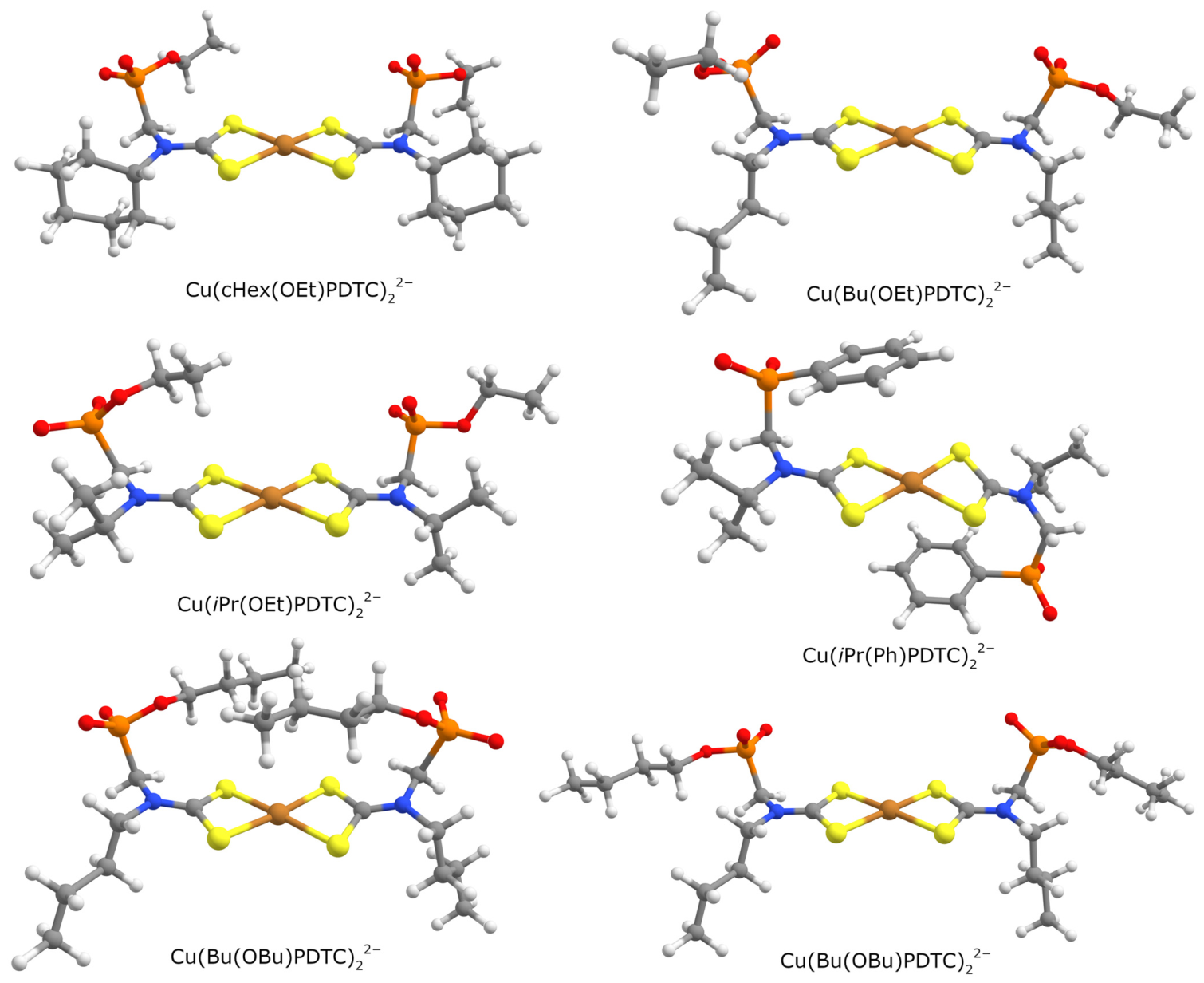
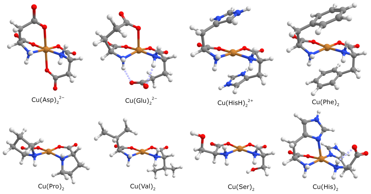
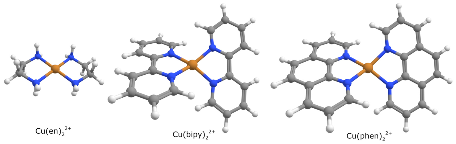
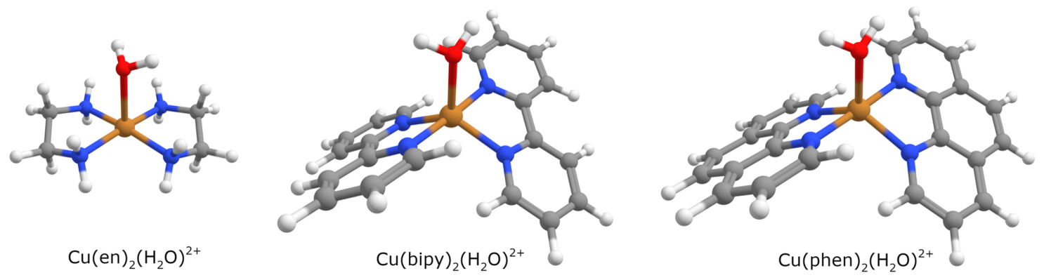
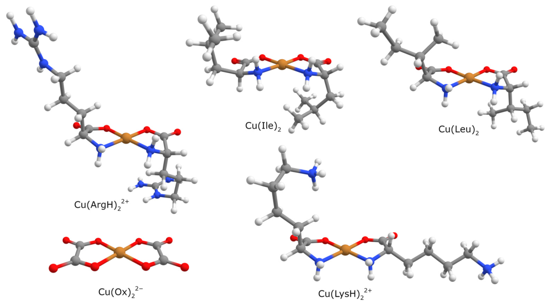
Some optimized structures are shown in Figure 1, Figure 2 and Figure 3 for complexes with phosphorylated dithiocarbamates, amino acids, and diimines, respectively (other structures with amino acids are given in Figure A1, Appendix A; more detailed information about complexes with phosphorylated dithiocarbamates can be found in the previously published work [17]).
As can be seen from Table 1, when aspartic acid is used as reference ligand, the constants for complexes with PDTC using the C-PCM model are significantly smaller than the experimental values, whereas values obtained using the SMD model are significantly larger than the measured constants. If the mean value of the two models’ results is taken, good agreement between calculated and experimental values is observed—the difference can be as small as a few tenths of a logarithmic unit. This is a highly interesting result, as the complexes with phosphorylated dithiocarbamates are structurally very different from the reference complex with aspartic acid (see Figure 1 and Figure 2): the coordinated atoms are not the same (only sulfur for PDTC; nitrogen and oxygen for Asp), the coordination arrangement differs (square planar for PDTC, distorted octahedral for Asp), and the chelate rings also differ (four-membered for PDTC; five- and six-membered for Asp). Only the charges of the ligands and complexes are identical.
When one of the PDTC ligands is used as reference, the calculated constants using the C-PCM and SMD models are much closer to the experimental values (Table 2). At the same time, the mean values are practically identical for cases using Asp (Table 1) and cHex(OEt)PDTC (Table 2) as reference ligands.
It should be noted that in the case of Bu(OBu)PDTC, two different sets of constants are obtained (see Table 1 and Table 2): in the first, the mean value is larger than the experimental result, whereas in the second, it is smaller. The two sets correspond to two different structures (Figure 1), which differ in the orientation of the BuO-substituents in the phosphonate fragments: in the first, the alkyl chains of neighboring ligands are located roughly parallel on one side of the copper plane (left structure in Figure 1); in the second, the BuO-groups are oriented outward, leaving the space above the CuS4-plane empty (right structure). The Gibbs free energy values of these two forms in solution differ significantly, so the constant can be overestimated or underestimated, whereas the mean value of them (21.87 for Table 1 and 21.78 tor Table 2) corresponds better to the experimental result. Therefore, for complexes with flexible side chains that can interact with each other, it is necessary to consider multiple optimized structures.
Returning to the data in Table 1, it can be seen that good agreement between calculated and experimental values is observed for some amino acid complexes (glutamic acid and phenylalanine), whereas for others, the values differ significantly (arginine, lysine, and serine). Inspection of the structures in Figure 2 and Figure A1 in comparison with data in Table 1 reveals the following observation: the differences between calculated and experimental values are small for complexes with direct axial coordination of ligand side chain (glutamic acid, similar to the reference aspartic acid) or with additional d-π-interaction with aromatic fragments (phenylalanine), whereas large discrepancies occur in the absence of such bonding. The possible reason for this is the some oversimplification of the given structures without axial interactions; copper(II) must be pentacoordinate with N,O-containing ligands [24,25], and an additional water molecule is necessary (see the next section).
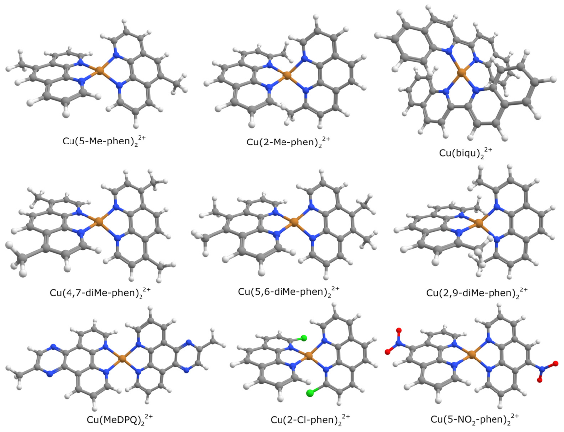
Additional attention in Table 1 is attracted by the significant difference (near 10 logarithmic units) between calculated and experimental values for bis-complexes with diimines. This discrepancy cannot be attributed to the non-planarity of the CuN4 arrangement in phenanthroline and bipyridine complexes (Figure 3), as the deviation for the ethylenediamine complex is similarly large, despite its nearly planar coordination geometry (Figure 3). A similar underestimation of the constant is observed for the complex with protonated histidine (Table 1). In this case, the ligand is neutral (zwitterionic form), and the complex carries a “+2” charge.
Therefore, the much more probable explanation for this discrepancy is the significant difference in charges of the ligands (neutral for the target; dianionic for the reference) and the complexes (investigated has “+2” charge; reference has “−2” charge). Consequently, the error likely stems from the differing solvation energy calculations for species with different charges, rendering the chosen reference ligand and complex inappropriate for this case. To address this issue, recalculation was performed using ethylenediamine (en) as reference ligand, and the results are presented in Table 3 (including additional substituted phenanthrolines and related ligands; structures are shown in Figure A2).
As can be seen from Table 3, much better agreement between calculated and experimental values is observed when en is used as the reference, with only a few exceptions. The first exception is the biquinolyl complex; however, its experimental constant differs significantly from those of related complexes (see Table 3). This discrepancy may arise from the experimental value itself, particularly considering the literature-reported stabilization of copper(I) relative to copper(II) in complex with this ligand [26]. The remaining two exceptions are the chloro- and nitro-substituted phenanthrolines, for which the calculations consistently underestimate the experimental values (at practically the same level for both ligands). This is likely due to altered solvation of the ligands and complexes upon introduction of electron-withdrawing groups into the aromatic system, so the reference without such substituents became inappropriate.
Interestingly, when ethylenediamine is used as the refence, the calculated constant for the complex with protonated histidine (Cu(HisH)22+ form) is in very good agreement with the experimental value (Table 3).
Based on these results, it can be concluded that obtaining accurate calculated constants requires the use of an appropriate reference complex that closely resembles the target complex.

2.2. Copper(II) Bis-Homoligand Complexes with Additional Water Molecules

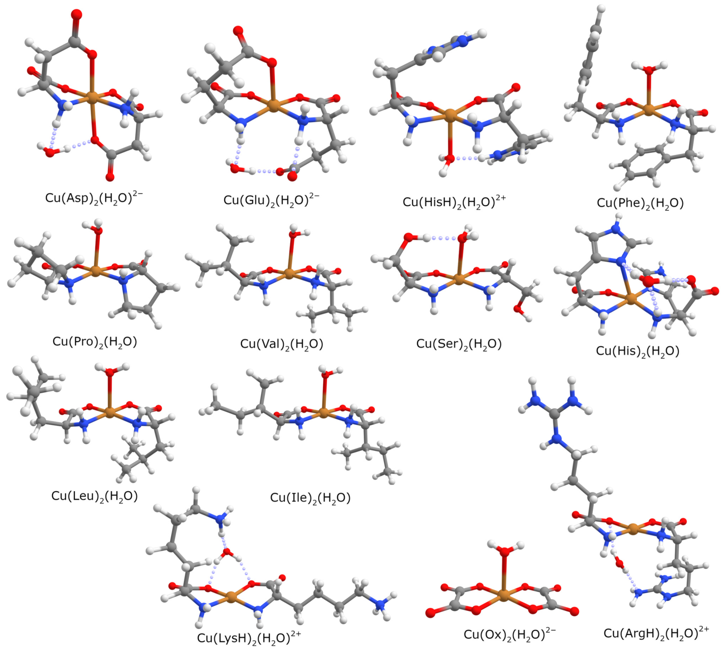
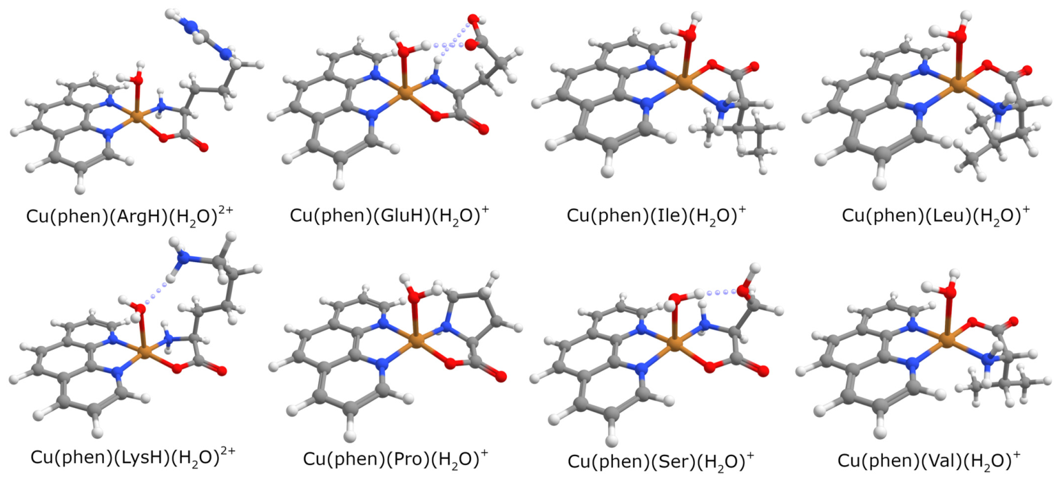
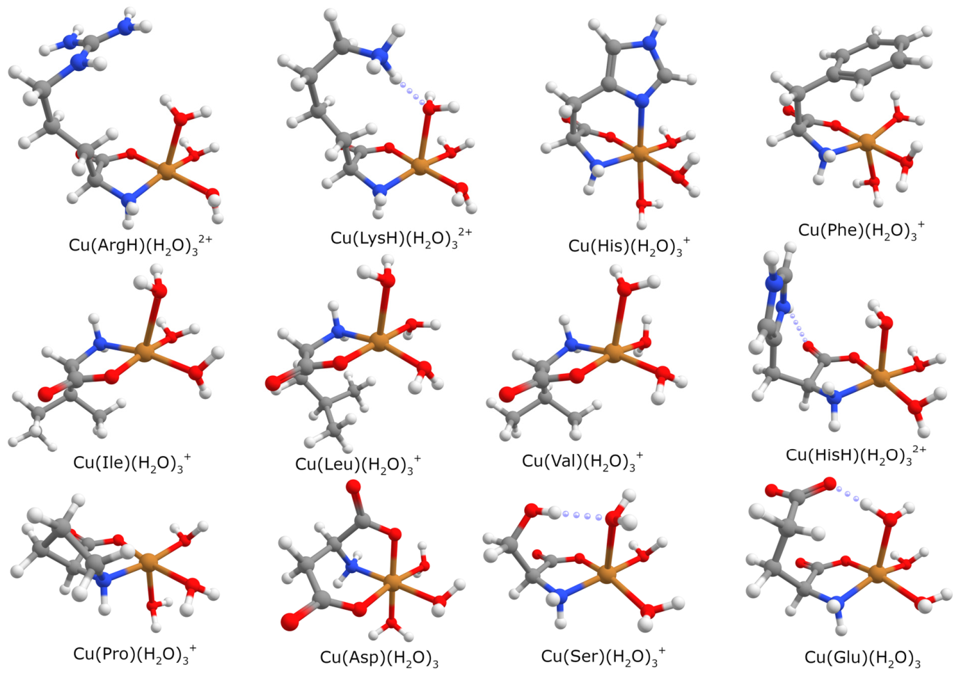
As was mentioned in the previous Section, copper(II) complexes with N,O-containing ligands are typically pentacoordinate. However, many structures presented in Figure 2, Figure 3, Figure A1, and Figure A2 exhibit only four-coordinate geometries. To make more realistic structures for all complexes (except those with PDTC, which adopt square-planar coordination [17]), an additional water molecule was added (where possible, it was initially placed in the axial position of the copper ion; otherwise, it was positioned near the amino/carboxy-groups). Optimized structures with an explicit water molecule for complexes with acids are shown in Figure 4, and recalculated formation constants are summarized in Table 4. In this case, leucine, an amino acid without a coordinated side chain, was selected as the reference.
As can be seen from Table 4, good agreement between the mean calculated and experimental values is primarily observed for copper(II) complexes containing an axially coordinated water molecule (see structures in Figure 4), namely those with isoleucine, oxalic acid, and serine. A good prediction for the isoleucine complex is expected when leucine is used as the reference. Meanwhile, the good agreement for serine (where additional hydrogen bond between the hydroxy group of the side chain and the axially coordinated water molecule is formed) and, especially for oxalic acid (which does not have side chains and differs in complex charge), is less straightforward. In all of these complexes, a square-pyramidal coordination arrangement is observed. However, the very similar complexes with proline and valine do not exhibit such good convergence between calculated and experimental data, which somewhat undermines the assumption of structural similarity between the studied and reference complexes.
As can be seen from Table 1 and Table 4, adding a water molecule to complexes with arginine and, especially, lysine reduces the discrepancy between calculated and experimental formation constants. However, good agreement is not achieved, likely due to hydrogen bonding between the side chains of these amino acids and the coordinated groups via the water molecule (Figure 4). Possibly, it is necessary to choose another reference in these cases.
Adding a water molecule to the complex with protonated histidine did not substantially alter the outcome; the discrepancy between calculated and experimental constants remains large (see Table 1 and Table 4). Conversely, the situation for the phenylalanine complex worsened, likely due to displacement of the phenyl ring from axial position of copper(II) upon water coordination. Furthermore, adding a water molecule to bis-complexes with aspartic and glutamic acids significantly worsens the results, increasing the discrepancy between calculated and experimental values to more than four logarithmic units (Table 4). The explanation about the dissimilarity of charges of the determined and reference complexes, which seems logical at first glance, is not suitable, since the complex with oxalic acid (similar in charge) shows good agreement in the same calculation scheme. Therefore, a more plausible explanation is that, in the cases of aspartic and glutamic acids, the additional water molecule does not coordinate to the copper ion but instead forms hydrogen bonds with the amino and carboxyl groups (Figure 4), thereby failing to maintain “similarity” with the reference complex.
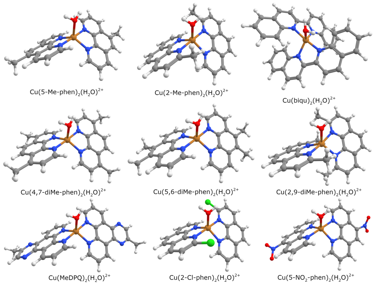
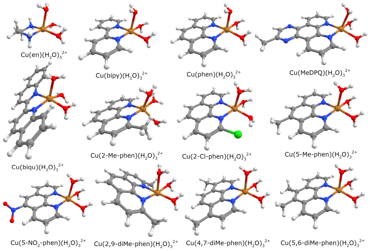
Re-evaluated data for diimine complexes in the presence of water molecule are presented in Table 5. Optimized structures are shown in Figure 5 and Figure A3, revealing that copper(II) is pentacoordinate in all cases. The coordination arrangement is a distorted trigonal bipyramid, with the exception of the ethylenediamine complex, which adopts a square-pyramidal geometry (Figure 5). Nevertheless, using en as the reference can give appropriate results for the calculated constants (Table 5). However, adding a water molecule to these complexes yields practically no improvement in the calculated constants. Comparing the data in Table 3 and Table 5 reveals that the deviations from experimental results are very similar, with only minor improvements observed for complexes with MeDPQ, 2,9-diMe-phen, and 5,6-diMe-phen. This contrasts sharply with amino acids complexes, where adding a water molecule can significantly improve the agreement between calculated and experimental data.
It should be noted that the formation constant for the bis-complex with protonated histidine can be properly predicted both with and without an explicit water molecule, using the ethylenediamine complex as the reference (see Table 3 and Table 5).

2.3. Copper(II) Heteroligand Complexes

The next objective of this study was to assess the possibility of calculating the constants for heteroligand complexes. Copper(II) compounds with diimines (1,10-phenanthroline and 2-methyldipyridoquinoxaline) and amino acids were selected for computational assessment, as these systems have been previously investigated in sufficient detail [18]. The calculation scheme remains the same; the difference lies in the increased number of interacting ligands compared to reaction (3), ranging from three to four depending on the formation reaction from the reference complex. Four ligands’ energies are necessary for the following reaction:
Cu(Lref1)(Lref2) + LA + LB = Cu(LA)(LB) + Lref1 + Lref2,
where Lref1 and Lref2 are the reference ligands; and LA and LB are the investigated ligands. When one ligand is not changed, then only two ligands’ energies are necessary:
Cu(L)(Lref) + LA = Cu(L)(LA) + Lref,
where ligand L is the same in the investigated and reference complexes. Another possible pathway for heteroligand complex formation uses a bis-homoligand compound as a reference; in this case, three ligands’ energies are necessary:
Cu(Lref)2 + LA + LB = Cu(LA)(LB) + 2Lref
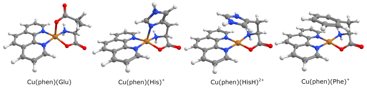
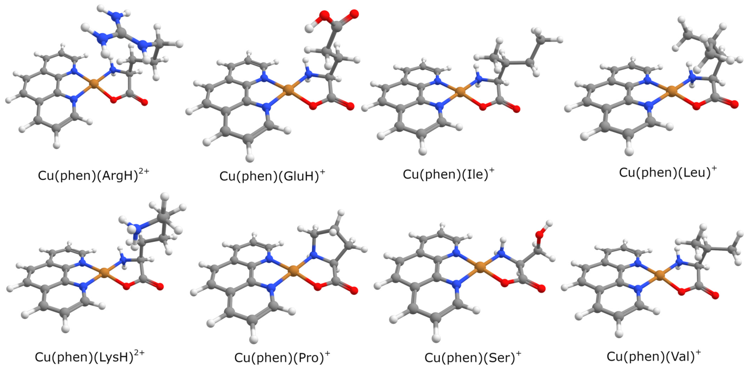
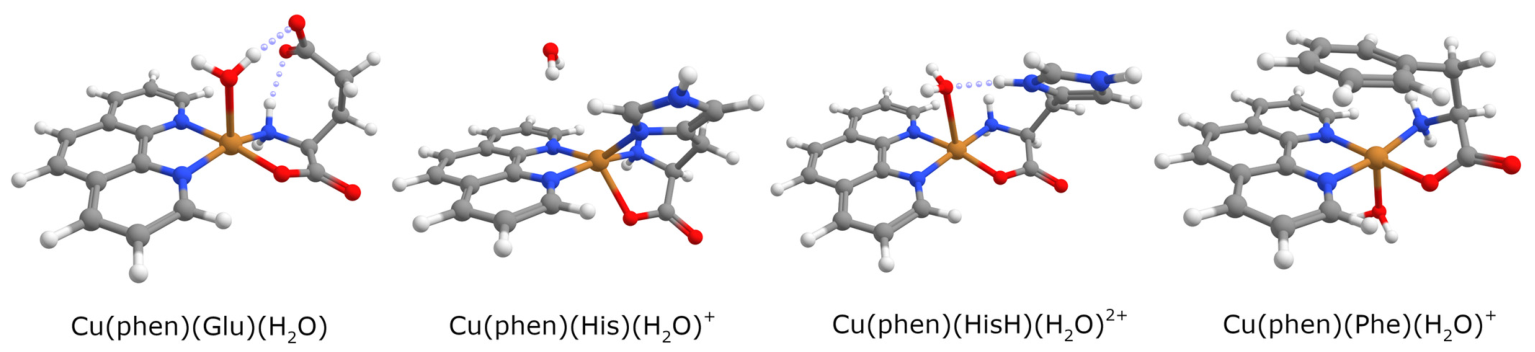
As observed in homoligand amino acid complexes (see data and discussion above), certain amino acids in heteroligand complexes can interact with the axial position of copper(II), making an additional water molecule unnecessary in these cases. Calculated constants for complexes with axial interactions are given in Table 6, and optimized structures are shown in Figure 6 for heteroligand complexes with phenanthroline (structures for complexes with MeDPQ are very similar and not presented).
As can be seen from Table 6, good agreement between calculated and experimental values is observed. Similar data for complexes lacking axial interaction and calculated without an explicit water molecule are presented in Table A1, with structures shown in Figure A4. Even this simplification of copper(II) coordination arrangement from square-pyramidal to square-planar yields relatively good agreement between predicted and measured values in certain cases (see Table A1).
Explicit water molecule addition gives square-pyramidal structures with axial H2O (optimized structures are shown in Figure 7) and improves the agreement between calculated and experimental formation constants (Table 7).
Conversely, adding water molecule to heteroligand complexes with Glu2−, His, HisH, and Phe results in a slight increase in differences between predicted and measured values (compare Table 6 and Table A2).
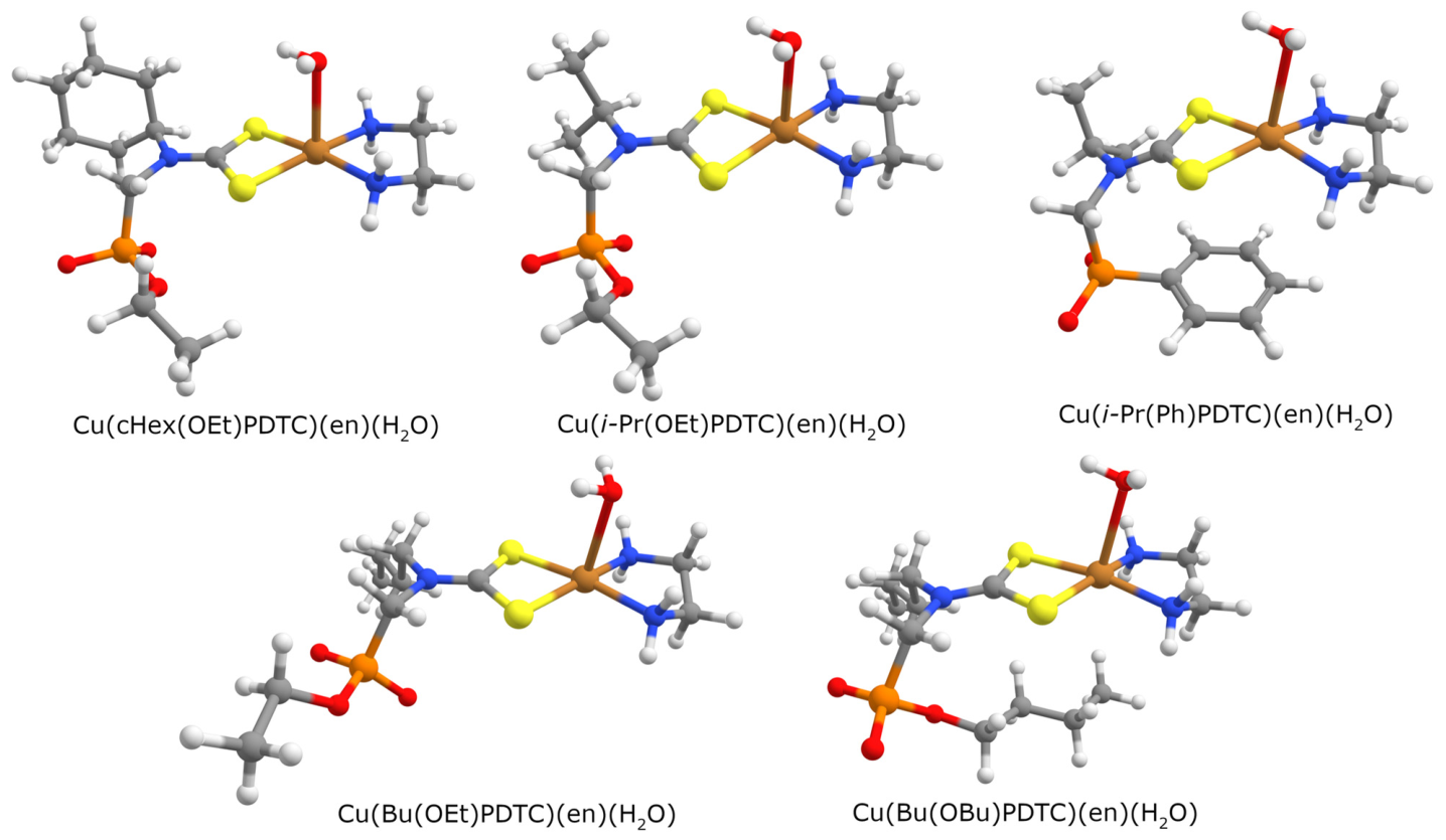
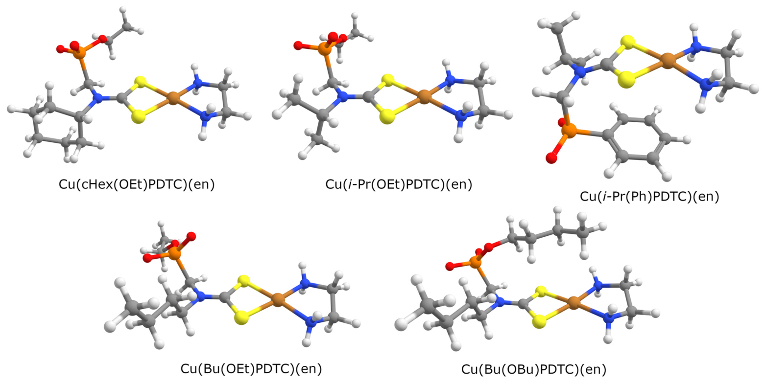
Formation constants for copper(II) heteroligand complexes with phosphorylated dithiocarbamates and ethylenediamine were also calculated. As these complexes are pentacoordinate (see Figure 8 and work [17]), a reference complex containing an axially coordinated water molecule should be used. Results of such calculations are presented in Table 8. As can be seen from the given data, relatively good agreement between experimental data and calculated values is observed. A significant discrepancy is observed only for the heteroligand complex with Bu(OBu)PDTC, which may be attributed to conformational flexibility, similar to that observed for the homoligand complex of this ligand (see Section 2.1).
Calculations for heteroligand complexes with PDTC without an explicit water molecule (structures in Figure A6) were also performed, with results presented in Table A3. However, the discrepancy between predicted and experimental values is larger than in the case including water (Table 8). This suggests that using “realistic” structures (square-pyramidal for the mentioned complexes, Figure 8) is preferable to simplified ones (square-planar, Figure A6), and that structural similarity may be more critical than charge similarity.
The data presented in this section provide evidence that the described method can also be applied to calculate formation constants for copper(II) heteroligand complexes.

2.4. Copper(II) Monoligand Complexes

Another question regarding the applicability of the proposed method is its use for determining the formation constants of copper(II) complexes containing a single organic ligand, with the remaining coordination sites occupied by water molecules. Mono complexes with amino acids and diimines were optimized (structures shown in Figure A7 and Figure A8), and calculated constants are presented in Table 9. Two reference complexes were used: a monoligand complex with leucine (for amino acids) and a compound with ethylenediamine (for diimines and histidine).
As can be seen from Table 9, relatively good agreement between experimental and calculated values is observed for many cases. The discrepancy is notable for amino acids with long side chains (arginine and lysine; reasons discussed above) and for acidic ligands (aspartic, glutamic, and oxalic acids). It was previously suggested that charge similarity is less critical for accurate predictions of bis-complexes (see Section 2.1); however, for mono-complexes with small, highly charged ligands, this may not hold true due to their higher charge density compared to complexes with two ligands.
The constants for complexes with chloro- and nitro-substituted phenanthrolines are again underestimated (similar to their bis-complexes; see Table 3 and Table 5). The distortion of the coordination arrangement for complexes with biqu, 2-Me-phen, and 2,9-diMe-phen (Figure A8) cannot explain the larger discrepancies between calculated and experimental values (Table 9), as the differences for complexes with phen and 4,7-diMe-phen are similarly large, despite significantly less distortion.
Based on the presented data, it can be concluded that the described method also works satisfactorily for monoligand complexes when an appropriate reference is used. Thus, the formation constants for various copper(II) complexes (mono- and bis-; homo- and heteroligand) with diverse organic ligands (such as amino acids and diimines) can be relatively accurately predicted using quantum-chemical calculations. The applicability of the described method to other complex formers merits further investigations.

2.5. Statistical Analysis

To evaluate the effectiveness of the approach used for averaging the stability constants obtained using the C-PCM and SMD models, a statistical analysis was performed using the mean error (ME), mean absolute error (MAE), and root mean squared error (RMSE) metrics, using the data from Table 1, Table 2, Table 3, Table 4, Table 5, Table 6, Table 7, Table 8, Table A1, Table A2 and Table A3. Before describing the obtained metrics, it is worth discussing the definition of the data sample for this statistical analysis. Since the primary and most powerful factor in obtaining close calculated constants in the calculation scheme used is the selection of the correct reference complex, the accuracy of the calculations using the models should be assessed only based on the sample of values for which the correct reference was used. Therefore, we introduced the selection criterion ∆lgβ between the experimental and model-averaged values. A level of ∆lgβ < 2 log. units was chosen as an indicator of the correct reference selection, taking into account possible deviations due to the accuracy of the experimental constants and the influence of conformers. The results obtained are presented in Table 10 (similar data for other values of the ∆lgβ criterion are given in Table A4).
According to the mean error data, the CPCM model exhibits a tendency to systematically underestimate values (ME = −0.900), while the SMD model, conversely, systematically overestimates them (ME = +0.615). Both models are characterized by a moderate error spread, as indicated by the RMSE/MAE ratio of ~1.38 for both models. Averaging the values obtained from the two models led to a significant improvement in calculation accuracy, mitigating the multidirectional bias of the solvation models. The MAE of the mean dataset was 0.837, demonstrating a 44.8% and 42.8% reduction in mean absolute error compared to CPCM and SMD, respectively. A significant increase in accuracy was recorded for the RMSE metric: the value decreased to 0.992, corresponding to a 52.3% and 51.1% reduction relative to the isolated models. The ratio of RMSE to MAE, which serves as an indicator of the homogeneity of the error distribution, is also shown to be decreased from ~1.38 to 1.19 (by ~14%). The convergence of these metrics toward unity indicates that the distribution of ensemble errors has become more homogeneous. The averaging procedure not only reduced the average magnitude of the errors but also mitigated the impact of outliers present in each of the baseline models individually.
The mutual compensation of systematic errors and the suppression of random errors make the use of averaged values a statistically sound and preferable approach, providing a significant increase in the reliability of the final results when selected an appropriate reference complex.
Statistical analysis of the effect of an explicit water molecule revealed that for a set of complexes in which none of the ligands interacts with the axial position of copper(II), calculations with an explicit water molecule reduced the MAE by ~35% (from 1.090 to 0.727) and the RMSE by ~29% (from 1.268 to 0.914) for the model-averaged value of the constant. We should clarify that complexes for which, in calculations with and without water, ∆lgβ > 2 between the experimental and model-averaged values were excluded from the set. However, when using the entire set (while maintaining the exclusion criterion of ∆lgβ > 2), the MAE and RMSE are almost identical, indicating that the axial water molecule reduces the accuracy for complexes in which the ligand side chains can interact with the axial position of copper(II). Such ligands, in our case, include, for example, Asp, Glu, His, and Phe. As a result, it can be concluded that the use of an explicit water molecule in the calculation can improve the accuracy of the calculation scheme, but it is necessary to clearly understand whether the coordinated ligands can interact with the axial position of copper.

3. Materials and Methods

Quantum-chemical calculations were performed using Orca program (version 6.1.0) [28,29] at the B3LYP/def2-TZVPPD level [30,31,32,33,34] with D3 dispersion correction [35,36] using the Becke–Johnson damping scheme. The C-PCM [37] and SMD [38] models were used to account for solvent effects. Optimizations in C-PCM and SMD models were made independently. Frequency calculations are made for all species, including ligands. Due to the presence of copper(II) unpaired electron, all calculations were made in an unrestricted Hartree–Fock scheme. SCF, grid, RI/auxiliary basis, and solvation settings were used as defaults. The Gibbs energies from the calculations were used “as is”. Initial structures for calculations were prepared using the Avogadro program (version 1.2.0) [39]. Chemcraft (version 1.8, build 814) [40] was used for viewing and visualizing calculation results.

4. Conclusions

Determining reliable stability constants for metal complexes using solely quantum chemical methods is a non-trivial task. The primary challenges lie in correctly identifying the structures actually present in solution, adequately describing the solvation energies of the complexes and ligands, and accurately reproducing the energies of coordination bonds. This paper proposes a multifactorial approach that enables the calculation of stability constants for copper(II) complexes with organic ligands that are reasonably close to experimental values.
A key element of the proposed approach is the use of a ligand-exchange reaction involving a reference complex for which the experimental stability constant is known. In this case, the calculation of the reaction ΔG leads to the partial cancellation of certain systematic errors. The most significant of these are errors arising from the calculation of the energy of small, highly polar species—primarily the copper ion and the water molecule (as in direct ligand-addition reactions)—as well as inaccuracies associated with the description of complex solvation. Utilizing the experimentally determined stability constant of the reference complex allows these contributions to be averaged out, thereby improving the agreement between calculated and experimental data.
Further improvement in the calculated constants was observed when averaging the results obtained from two solvation models: C-PCM and SMD. This effect appears to stem not only from the contribution of the CDS component in the SMD model but also from differences in the structural optimization of the compounds within the two models. It can be hypothesized that, in some instances, the actual solution-phase structure of the complex lies somewhere between the structures optimized using C-PCM and SMD. Although one model yielded values closer to experimental data for specific complexes, averaging the results led to improved agreement in the vast majority of cases. Nevertheless, such averaging does not entirely eliminate errors in the solvation description of various compounds; therefore, employing a reference ligand with similar solvation characteristics is crucial for obtaining more accurate constants.
The coordination similarity between the complex under study and the reference complex is an equally significant factor. For copper(II) complexes, using a square-planar complex (or one lacking distinct axial coordination) as a reference for calculating a pentacoordinate structure yields significantly poorer results than using a similar complex that includes an axially coordinated water molecule. In this context, distortion of the coordination center appears to be a less critical factor; for instance, the Cu(phen)22+ complex, which features a distorted equatorial plane, is well described using Cu(en)22+ as a reference, even though the latter has its four nitrogen atoms arranged in a virtually perfect plane. In this case, the accurate description of the solvation of the neutral ligands and the positively charged complex likely plays a more substantial role.
Ligands containing conformationally labile groups warrant special attention. The complex Cu(Bu(OBu)PDTC)22− demonstrates that limiting conformational states of the butyl fragments within the phosphonate group can yield calculated constant values that deviate from the experimental value by approximately two orders of magnitude in opposite directions. Consequently, when labile substituents are present, it is necessary to consider multiple potential structures and assess their impact on the final calculated constant. However, since conformational searching is a computationally intensive task, developing an optimal approach to account for conformers and isomers remains a subject for further research.
Based on the results obtained, the proposed approach for calculating stability constants can be formulated as follows:
  • A ligand-exchange reaction involving a reference complex—for which the stability constant was experimentally determined—is used as the computational model.
  • The reference ligand is selected to be structurally and solvationally similar to the ligand under study. Additionally, the reference complex must possess the same stoichiometry (including presence or absence coordinated water molecules) as the complex being characterized.
  • Calculations are performed using two solvation models (C-PCM and SMD), and the resulting values are averaged.
  • If the ligand contains conformationally labile groups, calculations are performed for several possible structures to assess the influence of the conformational state on the calculated stability constant.
Finally, it must be emphasized that the accuracy of the proposed approach depends largely on the reliability of the experimental constants used both for reference complexes and for comparison with calculated values. Stability constants depend, to varying degrees, on temperature and the background electrolyte. While a temperature of 25 °C is generally considered a standard condition, accounting for the background electrolyte presents a more complex challenge. The type and concentration of the background electrolyte can significantly influence the stability constant’s value. Furthermore, even under identical conditions, experimental values obtained by different research groups may differ due to variations in data processing and the software employed. For instance, the standard deviation for the Cu(en)22+ complex, calculated from data involving various background electrolytes and different research groups, is on the order of 0.4 logarithmic units. According to our assessment, published stability constant values for copper(II) amino acid complexes can differ by up to two logarithmic units; however, in most cases, the discrepancy does not exceed one logarithmic unit. Therefore, the selection of a reliable stability constant value for the reference complex is also key factor determining the reliability of the calculated result.
Further work in this area will focus on quantitatively calculating and assessing the «similarity parameter» between the determined and reference complexes. During quantum chemical calculations of the structure and delta-gamma of a complex, the output files contain many other parameters in addition to the total energy. A key to assessing «similarity» may be a model that includes the dielectric and CDS components of the solvation energy, the HOMO/LUMO, the spin distribution, bond lengths, and the bond and dihedral angles of both the complex and the ligands used.

Supplementary Materials

The following supporting information can be downloaded at https://www.mdpi.com/article/10.3390/inorganics14080202/s1. Archive contains xyz-files (with cartesian coordinates) for all optimized structures, including complexes and free ligands.

Author Contributions

Conceptualization, N.S.A. and N.Y.S.; methodology, N.Y.S. and M.S.B.; software, N.Y.S.; validation, N.S.A.; formal analysis, N.S.A., M.S.B. and N.Y.S.; investigation, N.S.A. and N.Y.S.; resources, N.Y.S.; data curation, N.S.A. and N.Y.S.; writing—original draft preparation, N.S.A. and N.Y.S.; writing—review and editing, M.S.B. and V.G.S.; visualization, N.S.A. and N.Y.S.; supervision, V.G.S.; project administration, N.S.A.; funding acquisition, N.Y.S. All authors have read and agreed to the published version of the manuscript.

Funding

The work of N. Yu. Serov was funded by financial support from the government assignment for the FRC Kazan Scientific Center of RAS, grant number 125030503189-7.

Institutional Review Board Statement

Not applicable.

Informed Consent Statement

Not applicable.

Data Availability Statement

The original contributions presented in this study are included in the article/Supplementary Materials. Further inquiries can be directed to the corresponding author.

Acknowledgments

The authors express sincere appreciation to Kazan Scientific Center of the Russian Academy of Science for providing the computational resources that enabled this work.

Conflicts of Interest

The authors declare no conflicts of interest. The funders had no role in the design of the study; in the collection, analyses, or interpretation of data; in the writing of the manuscript; or in the decision to publish the results.

Abbreviations

The following abbreviations are used in this manuscript:
AmAcamino acid
C-PCMconductor-like polarizable continuum model
DFTdensity functional theory
DiImdiimine
enethylenediamine
PDTCphosphorylated dithiocarbamate
Phen1,10-phenantroline
SMDsolvation model (based) on density

Appendix A

Figure A1. Optimized structures (B3LYP-D3/def2-TZVPPD level) of the copper(II) bis-complexes with animo acids in water (C-PCM model). Hydrogen atoms have white color; carbon—gray; nitrogen—blue; oxygen—red; and copper—brown.
Inorganics 14 00202 g0a1
Figure A2. Optimized structures (B3LYP-D3/def2-TZVPPD level) of the copper(II) bis-complexes with diimines in water (C-PCM model). Hydrogen atoms have white color; carbon—gray; nitrogen—blue; oxygen—red; chlorine—green; and copper—brown.
Inorganics 14 00202 g0a2
Figure A3. Optimized structures (B3LYP-D3/def2-TZVPPD level) of the copper(II) bis-complexes with diimines in the presence of additional water molecule (C-PCM model, water). Hydrogen atoms have white color; carbon—gray; nitrogen—blue; oxygen—red; chlorine—green; and copper—brown.
Inorganics 14 00202 g0a3
Table A1. Formation constants for copper(II) heteroligand complexes with phen/MeDPQ and amino acids, calculated using several references (designated at the corresponding block of the table). Solvent effects were treated in C-PCM and SMD models. Experimental values from the literature data are given for comparison.
Complexlgβ
(C-PCM)
lgβ
(SMD)
lgβ
(Mean 1)
lgβ
(Exp.)
∆lgβ 2
Reference—Cu(phen)(Leu)+, lgβ = 15.60 [18]
Cu(phen)(GluH)+11.049.7110.3710.96 [18]−0.59
Cu(phen)(Ile)+15.1215.4815.3015.61 [18]−0.31
Cu(phen)(Pro)+18.6416.6017.6216.18 [18]1.44
Cu(phen)(Ser)+14.7914.3614.5815.34 [18]−0.77
Cu(phen)(Val)+15.3514.4114.8815.75 [18]−0.87
Cu(MeDPQ)(GluH)+11.7710.0310.9010.05 [18]0.85
Cu(MeDPQ)(Ile)+15.1015.9115.5114.57 [18]0.94
Cu(MeDPQ)(Leu)+15.3515.8315.5914.54 [18]1.05
Cu(MeDPQ)(Pro)+18.0616.2617.1615.19 [18]1.97
Cu(MeDPQ)(Ser)+13.8813.8313.8514.41 [18]−0.56
Cu(MeDPQ)(Val)+14.5314.6814.6014.74 [18]−0.13
Reference—Cu(phen)(ArgH)2+, lgβ = 15.24 [18]
Cu(phen)(LysH)2+12.5814.1713.3815.31 [18]−1.93
Cu(MeDPQ)(ArgH)2+14.6516.0815.3614.22 [18]1.15
Cu(MeDPQ)(LysH)2+12.2013.6412.9214.29 [18]−1.37
1 Mean value between two models—C-PCM and SMD. 2 Differences between mean and experimental values.
Figure A4. Optimized structures (B3LYP-D3/def2-TZVPPD level) of the copper(II) heteroligand complexes with phen and amino acids (C-PCM model, water). Hydrogen atoms have white color; carbon—gray; nitrogen—blue; oxygen—red; and copper—brown.
Inorganics 14 00202 g0a4
Table A2. Formation constants for copper(II) heteroligand complexes with phen/MeDPQ and amino acids with explicit water molecule, calculated using several references (designated at the corresponding block of the table). Solvent effects were treated in C-PCM and SMD models. Experimental values from the literature data are given for comparison.
Complexlgβ
(C-PCM)
lgβ
(SMD)
lgβ
(Mean 1)
lgβ
(Exp.)
∆lgβ 2
Reference—Cu(phen)(Glu)(H2O), lgβ = 16.05 [18]
Cu(phen)(His)(H2O)+12.0315.3913.7116.56 [18]−2.85
Cu(phen)(Phe)(H2O)+13.1617.6215.3916.01 [18]−0.62
Cu(MeDPQ)(Glu)(H2O)15.4616.9116.1815.11 [18]1.07
Cu(MeDPQ)(His)(H2O)+12.7014.8213.7615.75 [18]−1.98
Cu(MeDPQ)(Phe)(H2O)+13.2117.4215.3214.29 [18]1.02
Reference—Cu(en)2(H2O)2+, lgβ = 20.03 [21]
Cu(phen)(HisH)(H2O)2+10.7811.0810.9312.74 [18]−1.81
Cu(MeDPQ)(HisH)(H2O)2+11.1211.3111.2211.73 [18]−0.51
1 Mean value between two models—C-PCM and SMD. 2 Differences between mean and experimental values.
Figure A5. Optimized structures (B3LYP-D3/def2-TZVPPD level) of the copper(II) heteroligand complexes with phen and amino acids with explicit water molecule (C-PCM model, water). Hydrogen atoms have white color; carbon—gray; nitrogen—blue; oxygen—red; and copper—brown.
Inorganics 14 00202 g0a5
Figure A6. Optimized structures (B3LYP-D3/def2-TZVPPD level) of the copper(II) heteroligand complexes with phosphorylated dithiocarbamates and ethylenediamine (C-PCM model, water). Hydrogen atoms have white color; carbon—gray; nitrogen—blue; oxygen—red; phosphorus—orange; sulfur—yellow; and copper—brown.
Inorganics 14 00202 g0a6
Table A3. Formation constants for copper(II) heteroligand complexes with phosphorylated dithiocarbamates and ethylenediamine, calculated using Cu(phen)(Glu) as reference (lgβ = 16.05 [18]). Solvent effects were treated in C-PCM and SMD models. Experimental values from the literature data are given for comparison.
Complexlgβ
(C-PCM)
lgβ
(SMD)
lgβ
(Mean 1)
lgβ
(Exp.)
∆lgβ 2
Cu(cHex(OEt)PDTC)(en)18.0924.0021.0521.33 [17]−0.28
Cu(iPr(OEt)PDTC)(en)17.5223.4020.4621.74 [17]−1.28
Cu(Bu(OEt)PDTC)(en)16.1321.7518.9421.32 [17]−2.38
Cu(Bu(OBu)PDTC)(en)17.0922.4719.7821.15 [17]−1.37
Cu(iPr(Ph)PDTC)(en)17.2624.2220.7421.72 [17]−0.98
1 Mean value between two models—C-PCM and SMD. 2 Differences between mean and experimental values.
Figure A7. Optimized structures (B3LYP-D3/def2-TZVPPD level) of the copper(II) monocomplexes with amino acids (C-PCM model, water). Hydrogen atoms have white color; carbon—gray; nitrogen—blue; oxygen—red; and copper—brown.
Inorganics 14 00202 g0a7
Figure A8. Optimized structures (B3LYP-D3/def2-TZVPPD level) of the copper(II) monocomplexes with diimines (C-PCM model, water). Hydrogen atoms have white color; carbon—gray; nitrogen—blue; oxygen—red; chlorine—green; and copper—brown.
Inorganics 14 00202 g0a8
Table A4. Statistical processing of deviations of the obtained stability constants of copper(II) bis-complexes for a data sample satisfying different criteria of ∆lgβ between the experimental and model-averaged values.
∆lgβ <MetricC-PCMSMDMean
1ME−1.0370.766−0.135
MAE1.4211.3740.498
RMSE2.1342.0950.576
RMSE/MAE1.5021.5251.158
2ME−0.9000.615−0.142
MAE1.5161.4630.837
RMSE2.0792.0300.992
RMSE/MAE1.3711.3881.185
3ME−1.0390.776−0.131
MAE1.7691.6611.033
RMSE2.4982.3431.263
RMSE/MAE1.4121.4111.223
4ME−1.0960.708−0.194
MAE1.8111.6801.077
RMSE2.5342.3511.333
RMSE/MAE1.3991.3991.237
5ME−0.9470.750−0.098
MAE1.9461.7611.210
RMSE2.6962.4271.582
RMSE/MAE1.3861.3781.307
6ME−1.0170.641−0.188
MAE2.0871.8851.367
RMSE2.8702.5791.874
RMSE/MAE1.3751.3681.371
All presented dataME−1.5930.250−0.671
MAE2.6062.1431.788
RMSE3.9332.9752.842
RMSE/MAE1.5091.3881.589

References

  1. Vukovic, S.; Hay, B.P.; Bryantsev, V.S. Predicting Stability Constants for Uranyl Complexes Using Density Functional Theory. Inorg. Chem. 2015, 54, 3995–4001. [Google Scholar] [CrossRef] [Scilit] [PubMed]
  2. Devarajan, D.; Lian, P.; Brooks, S.C.; Parks, J.M.; Smith, J.C. Quantum Chemical Approach for Calculating Stability Constants of Mercury Complexes. ACS Earth Space Chem. 2018, 2, 1168–1178. [Google Scholar] [CrossRef] [Scilit]
  3. Gutten, O.; Rulíšek, L. Predicting the Stability Constants of Metal-Ion Complexes from First Principles. Inorg. Chem. 2013, 52, 10347–10355. [Google Scholar] [CrossRef] [Scilit] [PubMed]
  4. Holland, J.P. Predicting the Thermodynamic Stability of Zirconium Radiotracers. Inorg. Chem. 2020, 59, 2070–2082. [Google Scholar] [CrossRef] [Scilit] [PubMed]
  5. Casasnovas, R.; Ortega-Castro, J.; Donoso, J.; Frau, J.; Muñoz, F. Theoretical Calculations of Stability Constants and pKa Values of Metal Complexes in Solution: Application to Pyridoxamine–Copper(Ii) Complexes and Their Biological Implications in AGE Inhibition. Phys. Chem. Chem. Phys. 2013, 15, 16303. [Google Scholar] [CrossRef] [Scilit] [PubMed]
  6. Bay, M.V.; Hien, N.K.; Thanh, H.K.; Nam, P.C.; Quang, D.T. Prediction of Stability Constants of Cu2+ Complexes with Organic Fluorescent Ligands Using Thermodynamic Cycle in Combination with DFT Theory and SMD Solvent Model. Hue Univ. J. Sci. Nat. Sci. 2020, 129, 15–23. [Google Scholar] [CrossRef] [Scilit]
  7. Gentry, B.M.; Choi, T.H.; Belfield, W.S.; Keith, J.A. Computational Predictions of Metal–Macrocycle Stability Constants Require Accurate Treatments of Local Solvent and pH Effects. Phys. Chem. Chem. Phys. 2021, 23, 9189–9197. [Google Scholar] [CrossRef] [Scilit] [PubMed]
  8. Lutoshkin, M.A. Solvation Effects on the Sustainability of Lanthanum Complexes. J. Phys. Chem. A 2025, 129, 5490–5498. [Google Scholar] [CrossRef] [Scilit] [PubMed]
  9. García Alejo, A.; De Silva, N.; Liu, Y.; Windus, T.L.; Pérez García, M. Solvent Phase Optimizations Improve Correlations with Experimental Stability Constants for Aqueous Lanthanide Complexes. Solvent Extr. Ion Exch. 2023, 41, 241–251. [Google Scholar] [CrossRef] [Scilit]
  10. Herchel, R.; Pražáková, M.; Drahoš, B. Computational Insight into Manganese(II) Complexes Comprising Macrocyclic Ligands for Magnetic Resonance Imaging. Dalton Trans. 2025, 54, 14495–14504. [Google Scholar] [CrossRef] [Scilit] [PubMed]
  11. Kostelnik, T.I.; Scheiber, H.; Cappai, R.; Choudhary, N.; Lindheimer, F.; Guadalupe Jaraquemada-Peláez, M.D.; Orvig, C. Phosphonate Chelators for Medicinal Metal Ions. Inorg. Chem. 2021, 60, 5343–5361. [Google Scholar] [CrossRef] [Scilit] [PubMed]
  12. Lutoshkin, M.A.; Kuznetsov, B.N.; Levdanskiy, V.A. The Interaction of Morin and Morin-5’-Sulfonic Acid with Lead(II): Study of the 1:1 Complex Formation Process in Aqueous Solution. Main Group Met. Chem. 2019, 42, 67–72. [Google Scholar] [CrossRef] [Scilit]
  13. Roy, L.E.; Martin, L.R. Theoretical Prediction of Coordination Environments and Stability Constants of Lanthanum Lactate Complexes in Solution. Dalton Trans. 2016, 45, 15517–15522. [Google Scholar] [CrossRef] [Scilit] [PubMed]
  14. Gutten, O.; Beššeová, I.; Rulíšek, L. Interaction of Metal Ions with Biomolecular Ligands: How Accurate Are Calculated Free Energies Associated with Metal Ion Complexation? J. Phys. Chem. A 2011, 115, 11394–11402. [Google Scholar] [CrossRef] [Scilit] [PubMed]
  15. Lutoshkin, M.A.; Petrov, A.I.; Malyar, Y.N.; Kazachenko, A.S. Interaction of Rare-Earth Metals and Some Perfluorinated β-Diketones. Inorg. Chem. 2021, 60, 3291–3304. [Google Scholar] [CrossRef] [Scilit] [PubMed]
  16. Purgel, M.; Schuur, J.H. First Principle Determination of Stability Constants of Metal Complexes by Cellmetry Method. Int. J. Quantum Chem. 2023, 123, e27214. [Google Scholar] [CrossRef] [Scilit]
  17. Aksenin, N.S.; Bukharov, M.S.; Rodionov, A.A.; Kuzin, Y.I.; Gubaidullin, A.T.; Islamov, D.R.; Shtyrlin, V.G.; Serov, N.Y. Copper Complexes with Phosphorylated Dithiocarbamates in Aqueous Media: Complexation, Structures and Redox Activity. Inorganics 2026, 14, 114. [Google Scholar] [CrossRef] [Scilit]
  18. Ermolaev, A.V.; Shtyrlin, V.G.; Gizatullin, A.I.; Zhernakov, M.A.; Serov, N.Y.; Urazaeva, K.V.; Bukharov, M.S.; Gilyazetdinov, E.M.; Islamov, D.R.; Rodionov, A.A.; et al. Development of Comprehensive Approaches to Characterizing CuII Complexes: Structures in Solution and Solid-state, Dynamic Behavior, and Bioactivity. ChemistrySelect 2023, 8, e202303333. [Google Scholar] [CrossRef] [Scilit]
  19. Yadava, P.C.; Ghose, A.K.; Yadava, K.L.; Dey, A.K. Stability Constants of Oxalate Complexes of Copper (II) and Nickel (II) by Paper Electrophoresis. Chromatographia 1976, 9, 410–412. [Google Scholar] [CrossRef] [Scilit]
  20. McBryde, W.A.E. A Critical Review of Equilibrium Data for Proton- and Metal Complexes of 1,10-Phenanthroline, 2,2’-Bipyridyl and Related Compounds; IUPAC Chemical Data Series; Pergamon Press: Oxford, UK, 1978. [Google Scholar]
  21. Maes, A.; Peigneur, P.; Cremers, A. Stability of Metal Uncharged Ligand Complexes in Ion Exchangers. Part 2.—The Copper+ethylenediamine Complex in Montmorillonite and Sulphonic Acid Resin. J. Chem. Soc. Faraday Trans. 1 1978, 74, 182. [Google Scholar] [CrossRef] [Scilit]
  22. Murphy, J.M.; Powell, B.A.; Brumaghim, J.L. Stability Constants of Bio-Relevant, Redox-Active Metals with Amino Acids: The Challenges of Weakly Binding Ligands. Coord. Chem. Rev. 2020, 412, 213253. [Google Scholar] [CrossRef] [Scilit]
  23. Bregier-Jarzebowska, R.; Gasowska, A.; Lomozik, L. Complexes of Cu(II) Ions and Noncovalent Interactions in Systems with L-Aspartic Acid and Cytidine-5′-Monophosphate. Bioinorg. Chem. Appl. 2008, 2008, 253971. [Google Scholar] [CrossRef] [Scilit] [PubMed]
  24. Bukharov, M.S.; Shtyrlin, V.G.; Mukhtarov, A.S.; Mamin, G.V.; Stapf, S.; Mattea, C.; Krutikov, A.A.; Il’in, A.N.; Serov, N.Y. Study of Structural and Dynamic Characteristics of Copper(Ii) Amino Acid Complexes in Solutions by Combined EPR and NMR Relaxation Methods. Phys. Chem. Chem. Phys. 2014, 16, 9411–9421. [Google Scholar] [CrossRef] [Scilit] [PubMed]
  25. Bukharov, M.S.; Shtyrlin, V.G.; Gilyazetdinov, E.M.; Serov, N.Y.; Madzhidov, T.I. Hydration of Copper(II) Amino Acids Complexes. J. Comput. Chem. 2018, 39, 821–826. [Google Scholar] [CrossRef] [Scilit] [PubMed]
  26. James, B.R.; Williams, R.J.P. 383. The Oxidation–Reduction Potentials of Some Copper Complexes. J. Chem. Soc. 1961, 164, 2007–2019. [Google Scholar] [CrossRef] [Scilit]
  27. Bottari, E.; Festa, M.R.; Jasionowska, R. Copper(II) Complexes with Aspartate and Glutamate. Polyhedron 1989, 8, 1019–1027. [Google Scholar] [CrossRef] [Scilit]
  28. Neese, F. The ORCA Program System. WIREs Comput. Molec. Sci. 2012, 2, 73–78. [Google Scholar] [CrossRef] [Scilit]
  29. Neese, F. Software Update: The ORCA Program System—Version 6.0. Wiley Interdiscip. Rev. Comput. Mol. Sci. 2025, 15, e70019. [Google Scholar] [CrossRef] [Scilit]
  30. Becke, A.D. Density-Functional Thermochemistry. III. The Role of Exact Exchange. J. Chem. Phys. 1993, 98, 5648. [Google Scholar] [CrossRef] [Scilit]
  31. Lee, C.; Yang, W.; Parr, R.G. Development of the Colle-Salvetti Correlation-Energy Formula into a Functional of the Electron Density. Phys. Rev. B 1988, 37, 785–789. [Google Scholar] [CrossRef] [Scilit] [PubMed]
  32. Weigend, F.; Ahlrichs, R. Balanced Basis Sets of Split Valence, Triple Zeta Valence and Quadruple Zeta Valence Quality for H to Rn: Design and Assessment of Accuracy. Phys. Chem. Chem. Phys. 2005, 7, 3297. [Google Scholar] [CrossRef] [Scilit] [PubMed]
  33. Weigend, F. Accurate Coulomb-Fitting Basis Sets for H to Rn. Phys. Chem. Chem. Phys. 2006, 8, 1057. [Google Scholar] [CrossRef] [Scilit] [PubMed]
  34. Rappoport, D.; Furche, F. Property-Optimized Gaussian Basis Sets for Molecular Response Calculations. J. Chem. Phys. 2010, 133, 134105. [Google Scholar] [CrossRef] [Scilit] [PubMed]
  35. Grimme, S.; Antony, J.; Ehrlich, S.; Krieg, H. A Consistent and Accurate Ab Initio Parametrization of Density Functional Dispersion Correction (DFT-D) for the 94 Elements H-Pu. J. Chem. Phys. 2010, 132, 154104. [Google Scholar] [CrossRef] [Scilit] [PubMed]
  36. Grimme, S.; Ehrlich, S.; Goerigk, L. Effect of the Damping Function in Dispersion Corrected Density Functional Theory. J. Comput. Chem. 2011, 32, 1456–1465. [Google Scholar] [CrossRef] [Scilit] [PubMed]
  37. Cossi, M.; Rega, N.; Scalmani, G.; Barone, V. Energies, Structures, and Electronic Properties of Molecules in Solution with the C-PCM Solvation Model. J. Comput. Chem. 2003, 24, 669–681. [Google Scholar] [CrossRef] [Scilit] [PubMed]
  38. Marenich, A.V.; Cramer, C.J.; Truhlar, D.G. Universal Solvation Model Based on Solute Electron Density and on a Continuum Model of the Solvent Defined by the Bulk Dielectric Constant and Atomic Surface Tensions. J. Phys. Chem. B 2009, 113, 6378–6396. [Google Scholar] [CrossRef] [Scilit] [PubMed]
  39. Hanwell, M.D.; Curtis, D.E.; Lonie, D.C.; Vandermeersch, T.; Zurek, E.; Hutchison, G.R. Avogadro: An Advanced Semantic Chemical Editor, Visualization, and Analysis Platform. J. Cheminform. 2012, 4, 17. [Google Scholar] [CrossRef] [Scilit] [PubMed]
  40. Chemcraft—Graphical Software for Visualization of Quantum Chemistry Computations. Version 1.8, Build 780. Available online: https://www.chemcraftprog.com (accessed on 22 July 2025).
Figure 1. Optimized structures (B3LYP-D3/def2-TZVPPD level) of the copper(II) bis-complexes with phosphorylated dithiocarbamates in water (C-PCM model). Hydrogen atoms have white color; carbon—gray; nitrogen—blue; oxygen—red; phosphorus—orange; sulfur—yellow; and copper—brown.
Inorganics 14 00202 g001
Figure 2. Optimized structures (B3LYP-D3/def2-TZVPPD level) of the copper(II) bis-complexes with amino acids in water (C-PCM model). Hydrogen atoms have white color; carbon—gray; nitrogen—blue; oxygen—red; and copper—brown.
Inorganics 14 00202 g002
Figure 3. Optimized structures (B3LYP-D3/def2-TZVPPD level) of the copper(II) bis-complexes with en, bipy, and phen in water (C-PCM model). Hydrogen atoms have white color; carbon—gray; nitrogen—blue; and copper—brown.
Inorganics 14 00202 g003
Figure 4. Optimized structures (B3LYP-D3/def2-TZVPPD level) of the copper(II) bis-complexes with animo acids in the presence of additional water molecule (C-PCM model, water). Hydrogen atoms have white color; carbon—gray; nitrogen—blue; oxygen—red; and copper—brown.
Inorganics 14 00202 g004
Figure 5. Optimized structures (B3LYP-D3/def2-TZVPPD level) of the copper(II) bis-complexes with en, bipy, and phen in the presence of additional water molecule (C-PCM model, water). Hydrogen atoms have white color; carbon—gray; nitrogen—blue; oxygen—red; and copper—brown.
Inorganics 14 00202 g005
Figure 6. Optimized structures (B3LYP-D3/def2-TZVPPD level) of the copper(II) heteroligand complexes with phen and amino acids (C-PCM model, water). Hydrogen atoms have white color; carbon—gray; nitrogen—blue; oxygen—red; and copper—brown.
Inorganics 14 00202 g006
Figure 7. Optimized structures (B3LYP-D3/def2-TZVPPD level) of the copper(II) heteroligand complexes with phen and amino acids with explicit water molecule (C-PCM model, water). Hydrogen atoms have white color; carbon—gray; nitrogen—blue; oxygen—red; and copper—brown.
Inorganics 14 00202 g007
Figure 8. Optimized structures (B3LYP-D3/def2-TZVPPD level) of the copper(II) heteroligand complexes with phosphorylated dithiocarbamates and ethylenediamine with explicit water molecule (C-PCM model, water). Hydrogen atoms have white color; carbon—gray; nitrogen—blue; oxygen—red; phosphorus—orange; sulfur—yellow; and copper—brown.
Inorganics 14 00202 g008
Table 1. Formation constants for copper(II) bis-homoligand complexes, calculated using aspartic acid as reference ligand (lgβ = 15.69 1). Solvent effects were treated in C-PCM and SMD models. Experimental values from the literature data are given for comparison.
Complexlgβ
(C-PCM)
lgβ
(SMD)
lgβ
(Mean 2)
lgβ
(Exp.)
∆lgβ 3
Cu(cHex(OEt)PDTC)22−16.4529.3522.9022.81 [17]0.09
Cu(iPr(OEt)PDTC)22−16.8028.5922.7022.87 [17]−0.17
Cu(Bu(OEt)PDTC)22−16.2027.3021.7522.08 [17]−0.33
Cu(Bu(OBu)PDTC)22− *16.9431.5824.2622.02 [17]2.24
Cu(Bu(OBu)PDTC)22− *11.6527.2919.4722.02 [17]−2.55
Cu(iPr(Ph)PDTC)22−17.3930.4423.9123.15 [17]0.76
Cu(ArgH)22+8.8811.3210.1013.40 [18]−3.30
Cu(Glu)22−15.3313.5114.4214.37 [18]0.05
Cu(His)214.5516.2915.4217.12 [18]−1.70
Cu(HisH)22+−4.521.45−1.538.71 [18]−10.24
Cu(Ile)212.0714.3813.2314.09 [18]−0.86
Cu(Leu)212.0913.6112.8514.46 [18]−1.61
Cu(LysH)22+4.969.457.2113.61 [18]−6.40
Cu(Ox)22−10.066.338.2010.00 [19]−1.90
Cu(Phe)212.4417.2214.8314.23 [18]0.60
Cu(Pro)217.9515.3216.6415.46 [18]1.18
Cu(Ser)210.3610.3810.3713.58 [18]−3.21
Cu(Val)211.7012.4912.0914.57 [18]−2.48
Cu(phen)22+0.585.443.0114.28 [18]−11.27
Cu(bipy)22+1.737.414.5713.80 [20]−9.23
Cu(en)22+7.2611.909.5820.03 [21]−10.45
1 Unpublished results, the value lies between two published data: 15.93 [22] and 15.35 [23]. 2 Mean value between two models—C-PCM and SMD. 3 Differences between mean and experimental values. * Data for the two structures shown in Figure 1.
Table 2. Formation constants for copper(II) bis-homoligand complexes, calculated using cHex(OEt)PDTC as reference ligand (lgβ = 22.81 [17]). Solvent effects were treated in C-PCM and SMD models. Experimental values from the literature data are given for comparison.
Complexlgβ
(C-PCM)
lgβ
(SMD)
lgβ
(Mean 1)
lgβ
(Exp.)
∆lgβ 2
Cu(iPr(OEt)PDTC)22−23.1622.0622.6122.87 [17]−0.16
Cu(Bu(OEt)PDTC)22−22.5720.7721.6722.08 [17]−0.41
Cu(Bu(OBu)PDTC)22−23.3125.0424.1822.02 [17]2.16
Cu(Bu(OBu)PDTC)22−18.0120.7519.3822.02 [17]−2.64
Cu(iPr(Ph)PDTC)22−23.7523.9023.8323.15 [17]0.68
1 Mean value between two models—C-PCM and SMD. 2 Differences between mean and experimental values.
Table 3. Formation constants for copper(II) bis-homoligand complexes with aromatic N-donor ligands, calculated using ethylenediamine as reference ligand (lgβ = 20.03 [21]). Solvent effects were treated in C-PCM and SMD models. Experimental values from the literature data are given for comparison.
Complexlgβ
(C-PCM)
lgβ
(SMD)
lgβ
(Mean 1)
lgβ
(Exp.)
∆lgβ 2
Cu(HisH)22+8.269.588.928.71 [18]0.21
Cu(bipy)22+14.5115.5315.0214.02 [20]1.00
Cu(biqu)22+13.5413.6113.587.73 [20]5.85
Cu(MeDPQ)22+10.2513.1711.7112.47 [18]−0.76
Cu(phen)22+13.3513.5713.4614.28 [18]−0.82
Cu(2-Me-phen)22+13.6114.0613.8413.8 [20]0.04
Cu(5-Me-phen)22+13.7514.7314.2415.02 [20]−0.78
Cu(2,9-diMe-phen)22+14.1514.4014.2711.7 [20]2.57
Cu(4,7-diMe-phen)22+16.0620.5518.3016.02 [20]2.28
Cu(5,6-diMe-phen)22+14.5214.6214.5715.7 [20]−1.13
Cu(2-Cl-phen)22+4.585.414.9910.45 [20]−5.46
Cu(5-NO2-phen)22+7.358.858.1013.47 [20]−5.37
1 Mean value between two models—C-PCM and SMD. 2 Differences between mean and experimental values.
Table 4. Formation constants for copper(II) bis-homoligand complexes with explicit water molecule, calculated using leucin as reference ligand (lgβ = 14.45 [18]). Solvent effects were treated in C-PCM and SMD models. Experimental values from the literature data are given for comparison.
Complexlgβ
(C-PCM)
lgβ
(SMD)
lgβ
(Mean 1)
lgβ
(Exp.)
∆lgβ 2
Cu(ArgH)2(H2O)2+11.1512.4911.8213.40 [18]−1.58
Cu(Asp)2(H2O)2−21.3618.4219.8915.69 34.20
Cu(Glu)2(H2O)2−20.3717.6919.0314.37 [18]4.66
Cu(His)2(H2O)18.8418.2818.5617.12 [18]1.44
Cu(HisH)2(H2O)2+−2.602.790.108.71 [18]−8.61
Cu(Ile)2(H2O)13.3414.4413.8914.09 [18]−0.20
Cu(LysH)2(H2O)2+11.0812.1811.6313.61 [18]−1.98
Cu(Ox)2(H2O)2−12.537.449.9810.00 [19]−0.02
Cu(Phe)2(H2O)14.0417.4715.7514.23 [18]1.52
Cu(Pro)2(H2O)20.3116.2618.2915.46 [18]2.83
Cu(Ser)2(H2O)13.8912.7513.3213.58 [18]−0.26
Cu(Val)2(H2O)13.0612.8712.9714.57 [18]−1.60
1 Mean value between two models—C-PCM and SMD. 2 Differences between mean and experimental values. 3 Unpublished results; the value lies between two published data: 15.93 [22] and 15.35 [23].
Table 5. Formation constants for copper(II) bis-homoligand complexes with aromatic N-donor ligands with explicit water molecule, calculated using ethylenediamine as reference ligand (lgβ = 20.03 [21]). Solvent effects were treated in C-PCM and SMD models. Experimental values from the literature data are given for comparison.
Complexlgβ
(C-PCM)
lgβ
(SMD)
lgβ
(Mean 1)
lgβ
(Exp.)
∆lgβ 2
Cu(HisH)2(H2O)2+7.069.168.118.71 [18]−0.60
Cu(bipy)2(H2O)2+14.8315.8915.3614.02 [20]1.34
Cu(biqu)2(H2O)2+12.2512.8212.547.73 [20]5.81
Cu(MeDPQ)2(H2O)2+11.8413.0112.4212.47 [18]−0.05
Cu(phen)2(H2O)2+13.1313.8713.5014.28 [18]−0.78
Cu(2-Me-phen)2(H2O)2+13.7913.7013.7413.8 [20]−0.06
Cu(5-Me-phen)2(H2O)2+14.0014.6614.3315.02 [20]−0.69
Cu(2,9-diMe-phen)2(H2O)2+11.8812.7812.3311.7 [20]0.63
Cu(4,7-diMe-phen)2(H2O)2+16.6319.7718.2016.02 [20]2.18
Cu(5,6-diMe-phen)2(H2O)2+15.1716.1415.6515.7 [20]−0.05
Cu(2-Cl-phen)2(H2O)2+5.195.485.3410.45 [20]−5.11
Cu(5-NO2-phen)2(H2O)2+8.449.548.9913.47 [20]−4.48
1 Mean value between two models—C-PCM and SMD. 2 Differences between mean and experimental values.
Table 6. Formation constants for copper(II) heteroligand complexes with phen/MeDPQ and amino acids, calculated using several references (designated at the corresponding block of the table). Solvent effects were treated in C-PCM and SMD models. Experimental values from the literature data are given for comparison.
Complexlgβ
(C-PCM)
lgβ
(SMD)
lgβ
(Mean 1)
lgβ
(Exp.)
∆lgβ 2
Reference—Cu(phen)(Glu), lgβ = 16.05 [18]
Cu(phen)(His)+15.6315.2615.4516.56 [18]−1.11
Cu(phen)(Phe)+13.8616.9115.3916.01 [18]−0.62
Cu(MeDPQ)(Glu)15.6516.2015.9315.11 [18]0.82
Cu(MeDPQ)(His)+15.4615.1515.3115.75 [18]−0.44
Cu(MeDPQ)(Phe)+13.5016.5915.0514.29 [18]0.76
Reference—Cu(en)22+, lgβ = 20.03 [21]
Cu(phen)(HisH)2+12.4814.2013.3412.74 [18]0.60
Cu(MeDPQ)(HisH)2+11.4913.7012.5911.73 [18]0.87
1 Mean value between two models—C-PCM and SMD. 2 Differences between mean and experimental values.
Table 7. Formation constants for copper(II) heteroligand complexes with phen/MeDPQ and amino acids with explicit water molecule, calculated using several references (designated at the corresponding block of the table). Solvent effects were treated in C-PCM and SMD models. Experimental values from the literature data are given for comparison.
Complexlgβ
(C-PCM)
lgβ
(SMD)
lgβ
(Mean 1)
lgβ
(Exp.)
∆lgβ 2
Reference—Cu(phen)(Leu)(H2O)+, lgβ = 15.60 [18]
Cu(phen)(GluH)(H2O)+9.278.618.9410.96 [18]−2.02
Cu(phen)(Ile)(H2O)+14.7715.4615.1215.61 [18]−0.49
Cu(phen)(Pro)(H2O)+17.4315.4716.4516.18 [18]0.27
Cu(phen)(Ser)(H2O)+14.6214.4014.5115.34 [18]−0.83
Cu(phen)(Val)(H2O)+14.7214.0414.3815.75 [18]−1.37
Cu(MeDPQ)(GluH)(H2O)+9.328.008.6610.05 [18]−1.39
Cu(MeDPQ)(Ile)(H2O)+14.7215.9915.3614.57 [18]0.79
Cu(MeDPQ)(Leu)(H2O)+15.4515.9815.7214.54 [18]1.18
Cu(MeDPQ)(Pro)(H2O)+16.9115.6216.2715.19 [18]1.08
Cu(MeDPQ)(Ser)(H2O)+13.6714.0613.8614.41 [18]−0.55
Cu(MeDPQ)(Val)(H2O)+14.5214.9014.7114.74 [18]−0.03
Reference—Cu(phen)(ArgH)(H2O)2+, lgβ = 15.24 [18]
Cu(phen)(LysH)(H2O)2+14.4214.6614.5415.31 [18]−0.77
Cu(MeDPQ)(ArgH)(H2O)2+15.2515.3915.3214.22 [18]1.10
Cu(MeDPQ)(LysH)(H2O)2+15.0314.3314.6814.29 [18]0.39
1 Mean value between two models—C-PCM and SMD. 2 Differences between mean and experimental values.
Table 8. Formation constants for copper(II) heteroligand complexes with phosphorylated dithiocarbamates and ethylenediamine, calculated using Cu(phen)(Leu)(H2O)+ as reference (lgβ = 15.60 [18]). Solvent effects were treated in C-PCM and SMD models. Experimental values from the literature data are given for comparison.
Complexlgβ
(C-PCM)
lgβ
(SMD)
lgβ
(Mean 1)
lgβ
(Exp.)
∆lgβ 2
Cu(cHex(OEt)PDTC)(en)(H2O)20.3924.3422.3721.33 [17]1.04
Cu(iPr(OEt)PDTC)(en)(H2O)19.8723.5421.7021.74 [17]−0.04
Cu(Bu(OEt)PDTC)(en)(H2O)18.3023.1620.7321.32 [17]−0.59
Cu(Bu(OBu)PDTC)(en)(H2O)19.0426.3422.6921.15 [17]1.54
Cu(iPr(Ph)PDTC)(en)(H2O)19.4224.9122.1721.72 [17]0.45
1 Mean value between two models—C-PCM and SMD. 2 Differences between mean and experimental values.
Table 9. Formation constants for copper(II) monoligand complexes, calculated using several references (designated at the corresponding block of the table). Solvent effects were treated in C-PCM and SMD models. Experimental values from the literature data are given for comparison.
Complexlgβ
(C-PCM)
lgβ
(SMD)
lgβ
(Mean 1)
lgβ
(Exp.)
∆lgβ 2
Reference—Cu(Leu)(H2O)3+, lgβ = 7.77 [18]
Cu(ArgH)(H2O)32+5.725.345.537.21 [18]−1.68
Cu(Asp)(H2O)312.5710.8711.728.40 [27]3.32
Cu(Glu)(H2O)311.5410.1010.828.10 [18]2.72
Cu(His)(H2O)3+9.679.559.619.39 [18]0.22
Cu(Ile)(H2O)3+7.608.267.937.64 [18]0.29
Cu(LysH)(H2O)32+3.855.184.517.36 [18]−2.85
Cu(Ox)(H2O)38.614.916.762.40 [19]4.36
Cu(Phe)(H2O)3+8.059.928.997.42 [18]1.57
Cu(Pro)(H2O)3+11.309.1910.248.39 [18]1.86
Cu(Ser)(H2O)3+6.746.956.847.38 [18]−0.54
Cu(Val)(H2O)3+7.756.937.347.92 [18]−0.58
Reference—Cu(en)(H2O)32+, lgβ = 10.72 [21]
Cu(HisH)(H2O)2+4.865.435.154.80 [18]0.35
Cu(bipy)(H2O)2+8.587.708.148.20 [20]−0.06
Cu(biqu)(H2O)2+3.792.072.934.27 [20]−1.34
Cu(MeDPQ) (H2O)2+7.736.837.287.75 [18]−0.07
Cu(phen)(H2O)2+7.677.117.398.35 [18]−0.96
Cu(2-Me-phen)(H2O)2+6.246.646.447.40 [20]−0.96
Cu(5-Me-phen)(H2O)2+7.997.947.978.55 [20]−0.58
Cu(2,9-diMe-phen)(H2O)2+2.065.463.765.20 [20]−1.44
Cu(4,7-diMe-phen)(H2O)2+9.0910.689.888.76 [20]1.12
Cu(5,6-diMe-phen)(H2O)2+8.648.778.708.71 [20]−0.01
Cu(2-Cl-phen)(H2O)2+1.891.641.765.07 [20]−3.31
Cu(5-NO2-phen)(H2O)2+5.284.985.137.60 [20]−2.47
1 Mean value between two models—C-PCM and SMD. 2 Differences between mean and experimental values.
Table 10. Statistical processing of deviations of the obtained stability constants of copper(II) bis-complexes for a data sample satisfying the criterion of ∆lgβ < 2 logarithmic units between the experimental and model-averaged values.
MetricC-PCMSMDMean
ME−0.9000.615−0.142
MAE1.5161.4630.837
RMSE2.0792.0300.992
RMSE/MAE1.3711.3881.185
Disclaimer/Publisher’s Note: The statements, opinions and data contained in all publications are solely those of the individual author(s) and contributor(s) and not of MDPI and/or the editor(s). MDPI and/or the editor(s) disclaim responsibility for any injury to people or property resulting from any ideas, methods, instructions or products referred to in the content.