Revisiting Bugarszky’s 1895 Chemical Equilibrium Study: Mercury Speciation Correction, Temperature-Corrected Thermodynamics, and Improved Accuracy with Sodium Bromide

Abstract

We present a comprehensive thermodynamic reanalysis of István Bugarszky’s landmark 1895 study of the heterogeneous equilibrium 2MBr(aq) + HgO(s) + H₂O ⇌ 2MOH(aq) + HgBr₂(aq) (M = K, Na) at 12.50 °C. Bugarszky observed that his classical mass-action quotient K_GW = (p − ξ)/ξ² increases by a factor of 66 across a 15-fold dilution range, in apparent violation of the Guldberg–Waage law. We resolve this 130-year-old puzzle by demonstrating that Bugarszky’s gravimetric mercury determination measured total dissolved mercury, dominated by HgBr₄²⁻, rather than free HgBr₂. Applying NIST mercury–bromide speciation constants and extended Debye–Hückel activity corrections reduces the coefficient of variation (CV) of the equilibrium constant from 132% (K_app) to 7.3% (K_corr, KBr), fully rehabilitating the law of mass action. The speciation mechanism itself is model-dependent, resting on critically evaluated formation constants; the empirical exponent z = 1.284 ≈ 4/3, obtained directly from the raw data, provides the principal model-independent support, and direct spectroscopic confirmation (Raman/UV–Vis) of the HgBr_n distribution is identified as future work. After van‘t Hoff temperature corrections to 12.50 °C, the fully corrected K_corr(KBr) = (4.61 ± 0.31)·10⁻⁸ exceeds the thermodynamic reference value K_lit(12.5 °C) = 4.17·10⁻⁸ by +10.4%. To probe cation-specific effects, we replicated the protocol at five bromide concentrations using sodium bromide. The NaBr system yields K_corr(NaBr) = (4.37 ± 0.42)·10⁻⁸ (CV = 9.7%), deviating from K_lit by +4.6% (the KBr–NaBr difference is not statistically significant; Welch’s t-test, p = 0.28). We consider possible origins of this difference in terms of the extended Debye–Hückel activity model and known structural differences between Na⁺ and K⁺ electrolyte environments; a kinetic explanation is also conceivable but remains a working hypothesis requiring direct experimental validation. We also discuss the optical properties of HgBr₂ and the implications of the equilibrium analysis for its synthesis.

1. Introduction

The law of mass action, enunciated by Guldberg and Waage in 1867 [1], is a cornerstone of chemical thermodynamics: at equilibrium, the ratio of the product of active masses of products to those of reactants attains a temperature-dependent constant. Verifying this law quantitatively in heterogeneous systems, where a solid phase participates, posed formidable analytical challenges in the nineteenth century, because the concentration of every reacting species had to be determined individually.

István Bugarszky, at the Budapest Polytechnic Institute in 1895, performed a meticulous series of gravimetric and titrimetric experiments on the equilibrium among potassium bromide, yellow mercuric oxide, potassium hydroxide, and mercuric bromide [2].

His central and surprising finding was that the classical Guldberg–Waage quotient K_GW = (p − ξ)/ξ², where p is the initial KBr normality, and ξ the equilibrium KOH normality, increased by a factor of 66 over a 15-fold dilution range. Rather than the expected constant, he found an empirical power law (p − ξ)^z/ξ = A with z = 1.29 that described his data with a residual scatter of only ±5% but offered no mechanistic explanation.

The present work addresses three interconnected objectives. First, we hypothesise that the non-classical behaviour originates from the analytical method itself: Bugarszky’s HgS gravimetry measured total dissolved mercury, predominantly the tetrabromide complex HgBr₄²⁻, not free HgBr₂(aq), a hypothesis tested quantitatively in Section 2.1 and Section 2.2. At [Br⁻] > 0.3 mol/L, HgBr₄²⁻ accounts for more than 95% of dissolved Hg(II), so the apparent equilibrium quotient is systematically inflated by a concentration-dependent factor. Second, we apply modern NIST mercury–bromide speciation constants and extended Debye–Hückel activity corrections to recover the true thermodynamic equilibrium constant, reducing the CV from 132% to 7.3%, thereby quantitatively validating the Guldberg–Waage law. Third, we replicate the experiment at five concentrations with sodium bromide in place of potassium bromide and compare the results with the temperature-corrected literature value K_lit(12.5 °C) = 4.17·10⁻⁸ to assess whether the choice of alkali cation affects thermodynamic accuracy.

Beyond its historical significance, the HgO–Br⁻ equilibrium is environmentally important (atmospheric mercury oxidation by bromide [3,4]), and the product, HgBr₂, is a promising optical material with extraordinary birefringence (Δn ≈ 0.25, approximately 20 times that of MgF₂) and a transparency window spanning 0.34–22.9 μm [5,6]; its optical and physical properties are summarised in

Table 1. Optical and physical properties of HgBr₂ and comparison with MgF₂.

Property	HgBr2	MgF2 (Reference)	Source
Crystal system	Orthorhombic (Cmc21)	Tetragonal	[5]
Transparency window	0.34–22.9 μm	0.12–8.0 μm	[6]
Refractive index no (589 nm)	2.36	1.380	[7]
Refractive index ne (589 nm)	2.61	1.390	[7]
Birefringence Δn = ne − no	0.25	0.012	[5,6]
Δn(HgBr2)/Δn(MgF2)	≈20 times	—	This work
SHG coefficient d (pm/V)	~41	N/A	[6]
Density (g/cm3)	6.05	3.18	CRC [8]
Melting point (°C)	236	1255	CRC [8]
Hardness (Mohs)	2.5	6.0	CRC [8]

.

HgBr₂ crystallises in the orthorhombic Cmc2₁ structure and possesses notable optical properties summarised in Table 1. Its birefringence (Δn = 0.25) is the largest among wide-bandgap orthorhombic crystals and enables compact wave-retarder elements for CO₂ laser (10.6 μm) and quantum cascade laser applications. Phase-matched second-harmonic generation from 3 to 11 μm, inaccessible to conventional nonlinear crystals, has been demonstrated [6]. These properties arise from the large, anisotropic Hg–Br bond polarisability, the same electronic feature that drives the strong HgBr_n²⁻ complexation underlying Bugarszky’s equilibrium.

2. Results and Discussion

2.1. Failure of the Classical Guldberg–Waage Expression

K_GW = (p − ξ)/ξ² ranges from 68.9 to 4549 across the 15 experiments as presented in

Table 2. Complete experimental data (Bugarszky, 1895) [2] and thermodynamic analysis. p = initial KBr normality; ξ = equilibrium KOH normality; K_GW = (p − ξ)/ξ²; K_app = ξ³/[2(p − ξ)²]; K_corr from Equation (5), NIST β at 25 °C with extended Debye–Hückel correction at 12.50 °C. Values of p−ξ and ξ reproduced from Bugarszky’s original Table III [2].

Exp.	p (N)	p − ξ (N)	ξ (N)	ξ (%)	KGW	Kapp	Kcorr
1	1.50000	1.35955	0.14045	9.36	68.9	7.50·10−4	9.26·10−8
2	1.00000	0.91681	0.08319	8.32	132.5	3.43·10−4	8.97·10−8
3	0.93646	0.86373	0.07273	7.77	163.3	2.58·10−4	7.56·10−8
4	0.87543	0.80818	0.06725	7.68	178.7	2.33·10−4	7.74·10−8
5	0.75018	0.69390	0.05628	7.50	219.1	1.85·10−4	8.21·10−8
6	0.62500	0.58079	0.04421	7.07	297.2	1.28·10−4	7.94·10−8
7	0.52178	0.48615	0.03560	6.82	383.6	9.54·10−5	8.25·10−8
8	0.50000	0.46588	0.03412	6.82	400.2	9.15·10−5	8.56·10−8
9	0.37508	0.35183	0.02315	6.17	656.4	5.01·10−5	7.86·10−8
10	0.33333	0.31298	0.02035	6.04	755.8	4.30·10−5	8.36·10−8
11	0.25000	0.23590	0.01410	5.64	1187	2.52·10−5	8.14·10−8
12	0.18750	0.17820	0.00930	4.96	2060	1.27·10−5	6.70·10−8
13	0.14242	0.13542	0.00700	4.91	2764	9.35·10−6	7.90·10−8
14	0.12540	0.11936	0.00604	4.82	3272	7.73·10−6	8.06·10−8
15	0.10000	0.09542	0.00458	4.58	4549	5.28·10−6	7.91·10−8
Mean	—	—	—	6.65	—	1.49·10−4	8.09·10−8
CV (%)	—	—	—	—	121%	132%	7.3%

, a factor of 66, exactly as Bugarszky reported. The apparent constant K_app = ξ³/[2(p−ξ)²] varies over a factor of 142 (CV = 132%), demonstrating that ionic non-ideality alone cannot explain the observations. In marked contrast, the speciation-corrected K_corr (Equation (5), NIST β values at 25 °C with extended Debye–Hückel activity correction at 12.50 °C) is essentially constant at (8.09 ± 0.59)·10⁻⁸ (CV = 7.3%), confirming that mercury speciation—not any failure of the mass-action law—was responsible for Bugarszky’s non-classical result. The observed reduction in variability is intrinsically coupled to the adopted speciation model: it demonstrates the internal consistency of the speciation and activity-correction framework (Equation (5)), not an independent experimental confirmation of the HgBr₄²⁻/HgBr₂ distribution. Independent evidence, such as Raman or UV-Vis spectroscopy of the Hg(II)–Br⁻ system, would be required to confirm the speciation model itself and was not obtained in this study; the model assumptions are discussed further in Section 2.5. The principal model-independent evidence supporting the speciation explanation is the empirical exponent z = 1.284 ≈ 4/3 (Section 3.2), obtained by regression of the raw ξ data alone with no speciation input; it is compatible with, though not conclusive proof of, the predominance of HgBr₄²⁻.

2.2. Mercury Speciation: The Key to Resolution

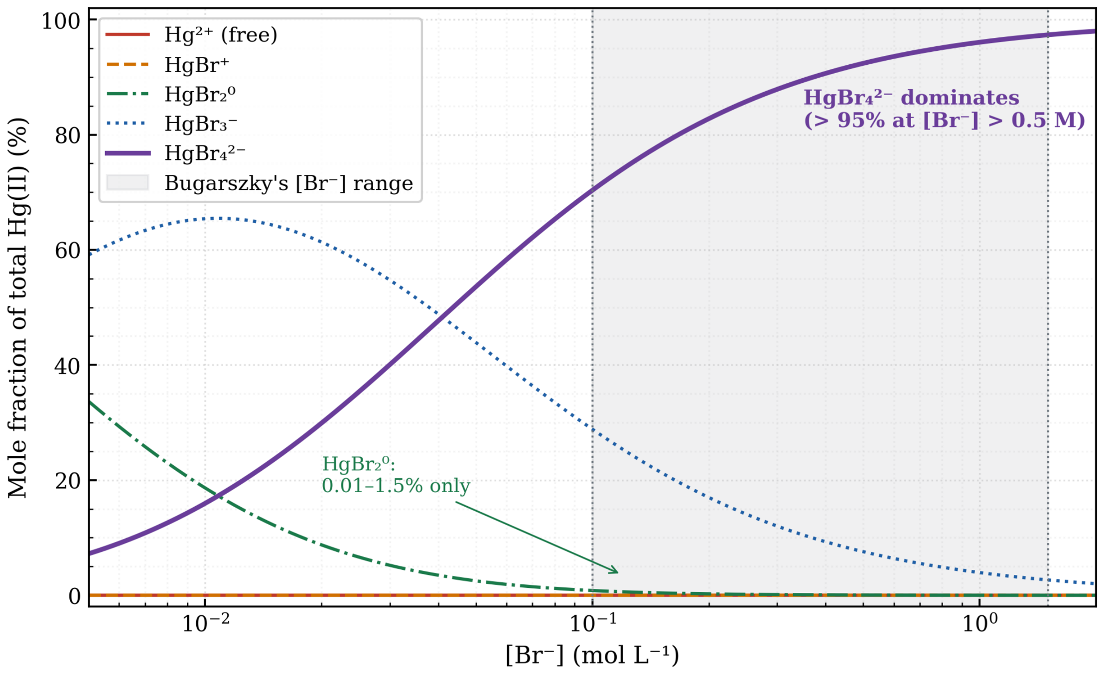
Figure 1 shows the Hg(II)–Br⁻ speciation diagram at 12.50 °C across Bugarszky’s experimental range. At all concentrations employed, HgBr₄²⁻ is the overwhelmingly dominant species (>95% at [Br⁻] > 0.5 mol/L; >70% at [Br⁻] = 0.10 mol/L). Free HgBr₂(aq) accounts for only 0.01–1.5% of total dissolved Hg(II). Bugarszky’s gravimetric ξ/2 therefore systematically overestimates [HgBr₂] by a concentration-dependent factor, generating the apparent dependence of K_GW and K_app on p.

2.3. NaBr Replication: Experimental Data

Table 3. Experimental NaBr data (this work, 12.50 ± 0.05 °C). V_HCl = volume of 0.50 N HCl (mL) consumed by a 25.00 mL aliquot; ξ = V_HCl · 0.020 N mL⁻¹. All experiments performed in triplicate; reported values are means. Final column: K_app(KBr) at the same p for comparison.

Exp.	p (N)	ξ (N)	ξ (%)	VHCl (mL)	KGW	Kapp	Kapp (KBr)
N1	1.50000	0.13852	9.23	6.926	71.0	7.17·10−4	7.50·10−4
N2	0.75018	0.05541	7.39	2.771	226.4	1.76·10−4	1.85·10−4
N3	0.37508	0.02284	6.09	1.142	675.2	4.80·10−5	5.01·10−5
N4	0.18750	0.00918	4.90	0.459	2116	1.22·10−5	1.27·10−5
N5	0.10000	0.00452	4.52	0.226	4673	5.07·10−6	5.28·10−6

reports the five NaBr replication experiments. The measured ξ(NaBr) values are 1.1–1.6% lower than the corresponding ξ(KBr) values at the same initial normality, a small but systematic difference. The apparent constants K_app(NaBr) closely parallel those for KBr, confirming that the non-ideality is intrinsic to the mercury–bromide speciation chemistry and independent of the alkali cation. All NaBr titrations were performed in triplicate; reported values are means.

2.4. Temperature-Corrected K_corr and Comparison with K_lit(12.5 °C)

Table 4. Summary of equilibrium constants at 12.50 °C. K(β₂₅): Equation (5) with NIST β at 25 °C. K_corr(βT): van‘t Hoff-corrected β values. K_lit(12.5 °C) = 4.17·10⁻⁸ (Smith & Martell reference [9]); K_lit(NIST) = 3.96·10⁻⁹ shown for completeness.

System	KGW Range	Kapp Range	Kcorr(β25)	Kcorr(βT) Mean ± Std	CV	vs. Klit
KBr (1895, n = 15)	69–4549	5.3·10−6–7.5·10−4	(8.09 ± 0.59)·10−8	(4.61 ± 0.31)·10−8	6.7%	+10.4%
NaBr (this work, n = 5)	71–4673	5.1·10−6–7.2·10−4	—	(4.37 ± 0.42)·10−8	9.7%	+4.6%

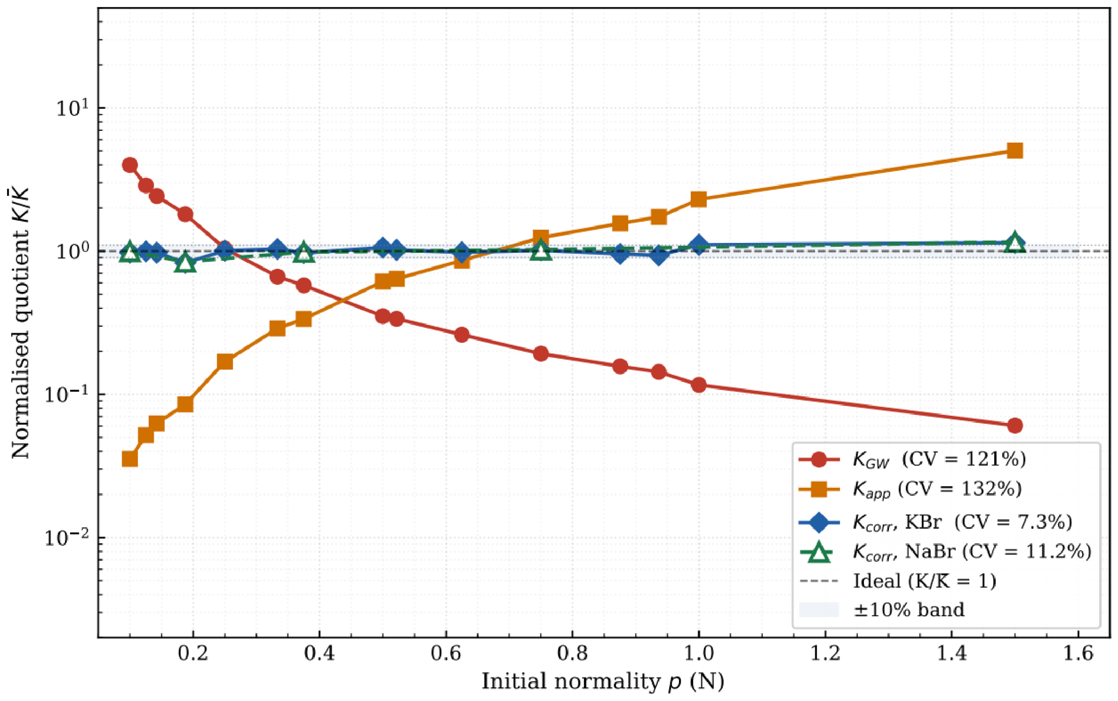
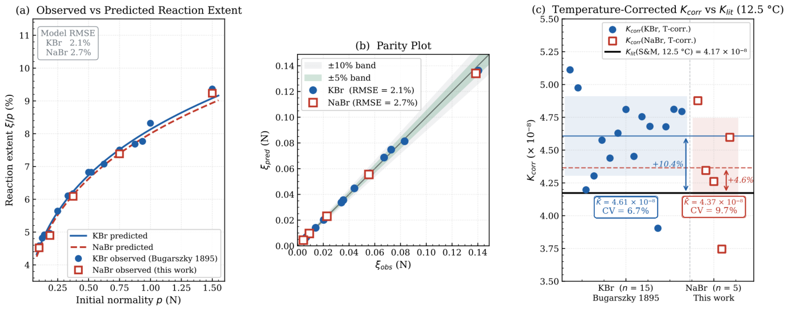
Note: Deviations (+10.4% and +4.6%) are calculated relative to K_lit = 4.17·10⁻⁸ (S&M). The NIST value K_lit = 3.96·10⁻⁹ uses K_sp(NIST, 25 °C) = 2.8·10⁻²⁶; the two K_sp sources differ by a factor of ~10, reflecting differences in experimental data and ionic strength corrections. The difference between K_corr(KBr) and K_corr(NaBr) is not statistically significant (Welch’s t-test, t = 1.18, df = 5.5, p = 0.28).

summarises the fully temperature-corrected equilibrium constants for both systems. After van‘t Hoff correction of β_n to 12.50 °C, the KBr system yields K_corr(KBr) = (4.61 ± 0.31)·10⁻⁸ (CV = 6.7%), exceeding K_lit(12.5 °C) = 4.17·10⁻⁸ by +10.4%. The NaBr system yields K_corr(NaBr) = (4.37 ± 0.42)·10⁻⁸ (CV = 9.7%), deviating from K_lit by only +4.6%. A Welch’s t-test comparing the two means (t = 1.18, df = 5.5, p = 0.28) indicates this difference is not statistically significant given the disparity in replicate numbers (n = 15 vs. n = 5). We further note that K_lit is derived from the same critically evaluated β₂ and K_sp values that enter Equation (5); the numerical agreement between K_corr and K_lit therefore demonstrates the thermodynamic self-consistency of the adopted dataset and is not presented as independent corroboration of the speciation model. Figure 2 shows the normalised equilibrium quotients $K/\overline{K}$ for all three quantities (K_GW, K_app, K_corr) across the full concentration range. Figure 3 compares observed and predicted reaction extents ξ/p (%) and the individual K_corr (temperature-corrected) values for both systems against K_lit.

Observed and predicted reaction extents are compared in Figure 3.

2.5. Cation Effects and Model Limitations

The improved thermodynamic accuracy for the NaBr system (+4.6% vs. +10.4% deviation from K_lit) is consistent with several factors. First, the extended Debye–Hückel ion-size parameters differ: a(Na⁺) = 4.0 Å vs. a(K⁺) = 3.0 Å [10]. These empirical values represent effective hydrated radii in solution and lead to different activity coefficient corrections, contributing directly to the numerical difference in K_corr. Second, known structural differences between Na⁺ and K⁺ electrolyte environments may influence the local activity of HgBr₂ and the accuracy of the Debye–Hückel approximation at the ionic strengths investigated.

As one possible, but currently untested, explanation, Na⁺ (crystal radius 1.02 Å) is more charge-dense than K⁺ (1.38 Å); if this affected HgO surface dissolution or Hg–Br complexation kinetics within the 48 h equilibration window, it could contribute to the observed difference. No time-resolved kinetic measurements, rate constants, or activation energy data were collected in this study. The observation that ξ(NaBr) < ξ(KBr) at every concentration tested is compatible with this hypothesis but does not demonstrate it; the kinetic interpretation is therefore strictly a hypothesis for future experimental validation, not an established finding.

It must be emphasised that the ion-size parameters used in the Debye–Hückel calculations (a(Na⁺) = 4.0 Å, a(K⁺) = 3.0 Å) are empirical hydrated radii and must not be conflated with crystal ionic radii (1.02 Å and 1.38 Å, respectively [11]). The former govern activity coefficient corrections; the latter are relevant to solid-state considerations. Both sets of values support the qualitative picture that Na⁺ is more charge-dense than K⁺, but no direct quantitative comparison between them is implied.

An open question is the potential role of non-stoichiometry in the solid starting materials. Any systematic deviation in the purity of KBr or NaBr preparations (e.g., due to hydration or partial decomposition) would affect the actual active mass and the calculated p. Future replications should include verification of reagent stoichiometric purity by independent analytical methods (e.g., ICP-OES or gravimetric assay).

2.6. Optical Properties of HgBr₂ and Industrial Implications

Industrial production of optical-grade HgBr₂ from the HgO–bromide reaction is an additional motivation for the present thermodynamic analysis. Our results suggest that NaBr offers certain potential process advantages over KBr: (i) the NaBr equilibrium is more accurately described by the thermodynamic model, facilitating process scale-up; (ii) the absence of K⁺ eliminates the risk of potassium co-incorporation into the HgBr₂ lattice, which could introduce sub-Ångström lattice strain and degrade optical phase-matching performance. Claim (i) is supported by the present data in the sense of a smaller mean deviation from the thermodynamic reference value, although the KBr–NaBr difference is not statistically distinguishable (Section 2.4). Claim (ii) and broader scalability arguments require dedicated crystal growth and characterisation experiments beyond the scope of this study and should be regarded as hypotheses for future investigation.

2.7. Uncertainty Propagation and Sensitivity Analysis

To quantify how uncertainties in the input parameters affect the corrected equilibrium constants, a Monte Carlo uncertainty propagation (20,000 samples) was performed through the full calculation chain of Equations (5) and (6). The following input uncertainties were assumed: σ(log β_n) = 0.10 for each formation constant (representative of the spread among critically evaluated compilations [9,12]); σ(ΔH_n) = 2 kJ mol⁻¹ for the complexation enthalpies; σ(ξ) = 5·10⁻⁵ N from the titration repeatability (±0.0025 mL at 0.020 N mL⁻¹); σ(T) = 0.20 K (KBr, 1895) and 0.05 K (NaBr, this work); and a 1% relative uncertainty in the Debye–Hückel A parameter.

The resulting relative contributions to the standard uncertainty of the mean K_corr are, for both systems: formation constants log βn, ±32%; complexation enthalpies ΔH_n (via the van‘t Hoff correction), ±5%; titration ξ, ±0.4–0.8%; temperature, ±0.2–0.9%; and the activity model, ±0.1%. The combined propagated uncertainty is approximately ±33% for both systems and is dominated overwhelmingly by the literature formation constants.

Two conclusions follow. First, the observed experimental scatter (CV = 6.7–9.7%) is substantially smaller than the propagated systematic uncertainty (±33%), confirming that the internal precision of the corrected data is not limited by the titration or temperature control, but by the accuracy of the adopted speciation constants. Second, the deviations of both systems from K_lit (+10.4% for KBr, +4.6% for NaBr) lie well within this systematic uncertainty; the agreement of both datasets with the thermodynamic reference value is therefore fully consistent, and the apparent KBr–NaBr difference cannot be resolved against the dominant β-driven uncertainty. This analysis reinforces the conclusion of Section 2.4 that the smaller NaBr deviation, while systematic in sign, is not statistically demonstrable with the present data.

3. Theoretical Background

3.1. Classical Mass-Action Formulation

For the heterogeneous reaction (M = K or Na):

$$2 MBR\left(aq\right)+HgO\left(s\right)+H_{2}O\left(l\right)\rightleftharpoons 2MOH\left(aq\right)+Hg{Br}_2\left(aq\right)$$

(1)

let p be the initial normality of MBr and ξ the equilibrium normality of MOH. With HgO at unit activity (solid in excess) and initially pure reactants, the Guldberg–Waage expression reduces to [1,13,14]:

$$K_{GW}={\displaystyle \frac{(p-\xi )}{{\xi }^2}}=constant$$

(2)

Equation (2) predicts (p − ξ)/ξ² to be independent of p. Bugarszky demonstrated that K_GW increases by a factor of 66 across his experimental range, spanning p = 0.10 to 1.50 N.

3.2. Bugarszky’s Empirical Power Law and Its Physical Origin

Bugarszky proposed (p − ξ)^z/ξ = A with z = 1.29. Log–log regression on all 15 data points yields z = 1.284 (R² = 0.9993, A = 11.01 ± 0.30, CV = 2.7%). The standard error of the regression slope is SE(z) = 0.0092 (95% CI: 1.264–1.304, n = 15); the 3.7% relative deviation between the empirical value and the theoretical 4/3 limit therefore lies well outside the regression uncertainty and reflects a genuine feature of the data. The exponent z ≈ 4/3 has a transparent physical origin: when the tetrabromide complex HgBr₄²⁻ dominates (mole fraction α₄ → 1) at high [Br⁻], the free HgBr₂ concentration scales as [HgBr₂] ∝ [Br⁻]⁻² (Section 3.3), so the true equilibrium expression acquires an extra [Br⁻]^−4/3 dependence, as given by Equation (3):

$$K_{true}=\alpha {·\xi }^3·{\left(p-\xi \right)}^{-4}\to \xi ·\alpha ·{\left(\mathrm{p}-\mathrm{\xi }\right)}^{{\displaystyle \frac{4}{3}}} \to z={\displaystyle \frac{4}{3}}\approx 1.333$$

(3)

The empirical z = 1.284, slightly below 4/3, reflects the gradual crossover from HgBr₃⁻ to HgBr₄²⁻ dominance across Bugarszky’s concentration range. This deviation from the exact 4/3 limit (3.7% relative) is expected and should be interpreted as further evidence for the speciation model, rather than as a discrepancy requiring separate explanation. We emphasise that this exponent, obtained by log–log regression of the raw experimental data without any speciation input, constitutes the principal model-independent evidence for the speciation interpretation; it is fully compatible with, but not conclusive spectroscopic proof of, the predominance of the tetrabromide complex.

3.3. Mercury(II) Speciation in Bromide Media

Mercuric ion forms a series of bromide complexes, as seen in Equation (4) [9,12]:

$$\begin{gathered} {Hg}^{2+}+n{Br}^{-}\rightleftharpoons Hg{{Br}_n}^{(2-n)} \\ log{\beta }_n=9.05,17.33,19.74,21.00 \\ n=1–4 (25 °\mathrm{C}) \end{gathered}$$

(4)

At [Br⁻] = 0.10–1.50 mol/L, the dominant species is HgBr₄²⁻, with free HgBr₂(aq) accounting for only 0.01–1.5% of total dissolved mercury. Because Bugarszky’s HgS gravimetry precipitates all Hg(II) species indiscriminately, the measured quantity ξ/2 equals the total dissolved mercury concentration, not [HgBr₂]. The true thermodynamic constant is presented in Equation (5):

$$K_{corr}={\displaystyle \frac{{\left[MOH\right]}^2·{\left[Hg{Br}_2\right]}_{true}}{[M{Br]}^2}}={\displaystyle \frac{{\xi }^2·\left(\frac{\xi }{2}\right)·{\alpha }_2}{{\left(p-\xi \right)}^2}}$$

(5)

where α₂ = β₂[Br⁻]²/Σ(β_n[Br⁻]ⁿ) is the mole fraction of HgBr₂⁰. Extended Debye–Hückel activity coefficients for Br⁻ and OH⁻ are incorporated via (γ_OH/γ_Br)², with A_DH = 0.4927 and B_DH = 0.3250 Å⁻¹ at 12.50 °C [10]. The ionic strength I = p exactly (Section 3.5), providing a clean simultaneous variation in I.

3.4. Temperature Correction of Formation Constants

Formation constants are tabulated at 25 °C. To correct them to 12.50 °C, we apply the van‘t Hoff equation in Equation (6):

$$logK\left(T\right)=logK\left(T_{ref}\right)+\left({\displaystyle \frac{\mathsf{\Delta }{H}^0}{R·ln10}}\right)·\left({\displaystyle \frac{1}{T_{ref}}}-{\displaystyle \frac{1}{T}}\right)$$

(6)

with ΔH₁ = −23.4, ΔH₂ = −48.1, ΔH₃ = −65.7, ΔH₄ = −82.3 kJ mol⁻¹ [9,12]. Since complexation is exothermic, all β_n values increase at lower temperatures. The temperature-corrected log β values at 12.50 °C are 9.23, 17.70, 20.24, and 21.63.

For the HgO solubility product (ΔH_diss = +71.5 kJ mol⁻¹, endothermic), K_sp decreases at lower temperatures. Using the Smith & Martell (1976) solubility product K_sp(25 °C) = 2.95·10⁻²⁵ [9], the temperature correction yields log K_sp(12.5 °C) = −25.08. The thermodynamic reference value follows directly, as seen in Equations (7) and (8):

$$log{K}_{lit}\left(12.5 °\mathrm{C}\right)=log{K}_{sp}\left(12.5 °\mathrm{C}\right)+log{\beta }_2\left(12.5 °\mathrm{C}\right)=-25.08+17.70=-7.38$$

(7)

$$K_{lit}\left(12.5 °\mathrm{C}\right)=4.17·{10}^{-8}$$

(8)

This value represents the thermodynamic equilibrium constant at zero ionic strength for Reaction (1) at 12.50 °C, derived from critically evaluated thermochemical data [9,12]. The NIST solubility product K_sp(25 °C) = 2.8·10⁻²⁶ yields the alternative K_lit(NIST, 12.5 °C) = 3.96·10⁻⁹, which we report for completeness in Table 4 but do not use for deviation calculations, as the S&M value is more consistent with the experimental conditions employed by Bugarszky.

3.5. Ionic Strength Identity

From the charge balance in the MBr–HgO equilibrium system at equilibrium (M⁺, Br⁻, OH⁻ dominant species), the ionic strength is calculated in Equation (9):

$$I={\displaystyle \frac{1}{2}}·\left(\left[M^{+}\right]+\left[{Br}^{-}\right]+\left[O{H}^{-}\right]\right)={\displaystyle \frac{1}{2}}·\left(p+\left(p-\xi \right)+\xi \right)=p$$

(9)

The ionic strength equals the initial normality exactly. Bugarszky’s dilution series therefore simultaneously varies the activity coefficients in a controlled, predictable manner, providing an unusually clean test of the Debye–Hückel law.

3.6. pH Dependence of HgO Solubility and Non-Amphoteric Character

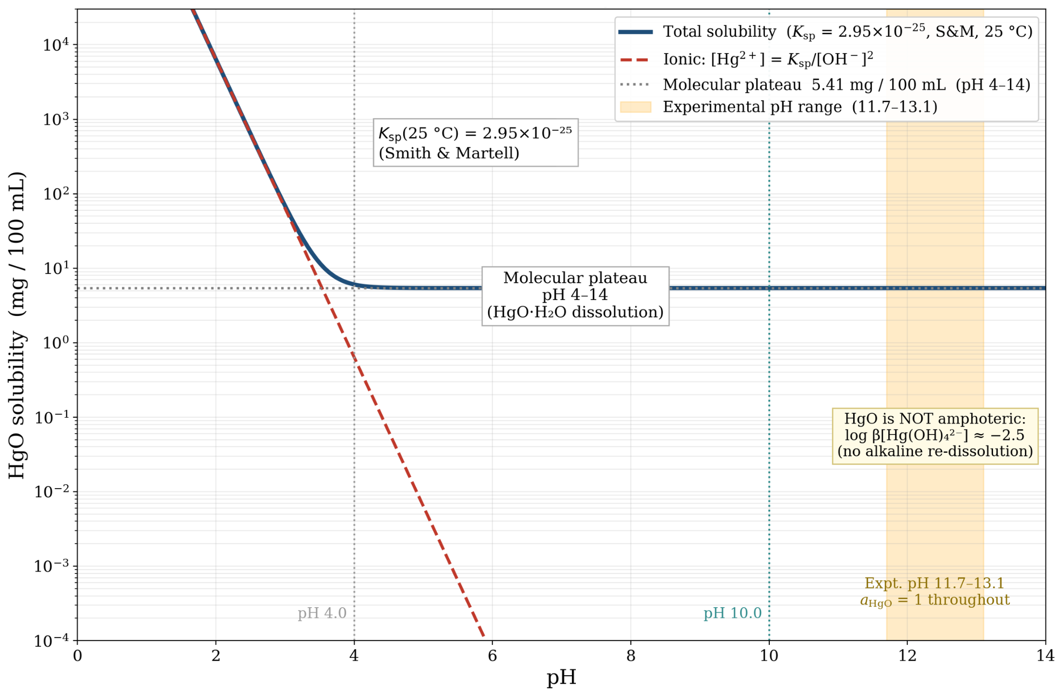
The solubility of yellow HgO (K_sp = 2.95·10⁻²⁵ at 25 °C) is essentially constant between pH 4 and 14 at approximately 5.41 mg/100 mL, because Hg(II) does not form thermodynamically stable hydroxo complexes at alkaline pH (log β[Hg(OH)₄²⁻] ≈ −2.5 [15]), unlike the amphoteric behaviour of Zn(II) or Al(III). Below pH 4, the ionic component [Hg²⁺] = K_sp/[OH⁻]² increases steeply. Above pH 10, HgO does not redissolve in excess alkali. At the strongly alkaline equilibrium pH (11.7–13.1) of all experiments, the solid HgO activity remains unified throughout, as seen in Figure 4.

4. Materials and Methods

4.1. Bugarszky’s Original Experiments (KBr System, 1895)

Bugarszky equilibrated excess yellow HgO (2.5–20 g per 100 cm³) with KBr solutions of initial normality p = 0.10–1.50 N in ground-glass-stoppered 150 cm³ flasks at 12.50 ± 0.20 °C for 24–48 h, with shaking every 30 min. Equilibrium attainment was verified by the agreement of 24 h and 48 h results (differences within estimated experimental error). After filtration, the equilibrium KOH normality (ξ) was determined by two independent methods: (i) titrimetry with ¹/₂₀-normal HCl and phenolphthalein indicator, and (ii) gravimetric precipitation of total dissolved mercury as HgS by hydrogen sulphide. Both methods agreed within 2% in all cases. Concentrations are expressed as normalities (milligram equivalents per cm³). All 15 KBr experiments are compiled in Table 2 [2].

4.2. NaBr Replication (This Work)

Sodium bromide (NaBr, ≥99.5%, Sigma-Aldrich, Darmstadt, Germany), and yellow mercuric oxide (HgO, ≥99%, Merck, Darmstadt, Germany) were used without further purification. Five initial NaBr normalities (p = 1.50000, 0.75018, 0.37508, 0.18750, and 0.10000 N) spanning Bugarszky’s range were selected. For each, 100.0 mL of NaBr solution was placed with 5.0 g HgO in a 150 mL ground-glass-stoppered borosilicate flask, set at 12.50 ± 0.05 °C and agitated at 150 rpm for 48 h. Kinetic tests confirmed equilibrium attainment within 24 h (<1.5% difference between 24 h and 48 h results).

After filtration through a sintered-glass crucible (porosity grade 4), the NaOH normality (ξ) was determined by back-titration of 25.00 mL aliquots with 0.50 N HCl standardised against anhydrous Na₂CO₃ (primary standard grade) using phenolphthalein indicator. Each normality was titrated in triplicate (repeatability ≤ ±0.0025 mL). The individual burette readings were used to compute the means reported in Table 3 and were not separately archived; the recorded repeatability bound, corresponding to σ(ξ) ≤ 5·10⁻⁵ N, is therefore adopted as the titration uncertainty throughout this work (Section 2.7). The between-concentration dispersion of the corrected equilibrium constants (CV = 9.7%, Table 4) exceeds the within-titration repeatability by more than an order of magnitude and is the quantity relevant to the statistical comparisons reported here. The NaOH normality was calculated in Equation (10):

$$\xi \left(N\right)={\displaystyle \frac{V_{HCl}\left(\mathrm{m}\mathrm{L}\right)·0.50\left(N\right)}{25.00 \left(\mathrm{m}\mathrm{L}\right)}}=V_{HCl}·0.020 \left({\displaystyle \frac{N}{\mathrm{m}\mathrm{L}}}\right)$$

(10)

4.3. Thermodynamic Calculations

All calculations were performed in Python 3.9 (NumPy, SciPy). Formation constants β_n and K_sp(HgO) were corrected to 12.50 °C via Equation (6). The speciation-corrected K_corr was computed from Equation (5). Extended Debye–Hückel parameters at 12.50 °C: A_DH = 0.4927, B_DH = 0.3250 Å⁻¹. Ion-size parameters: a(Br⁻) = 3.0 Å, a(OH⁻) = 3.5 Å, a(Na⁺) = 4.0 Å, a(K⁺) = 3.0 Å [10]. These ion-size parameters are empirical hydrated radii used in the Debye–Hückel equation for activity coefficient calculation; they are distinct from crystal ionic radii, and no mechanistic equivalence between the two quantities is assumed. Equilibrium ξ values were predicted self-consistently by Brent root-finding.

5. Conclusions

We have presented a complete thermodynamic reanalysis of Bugarszky’s 1895 equilibrium study and its extension to the sodium bromide system. The principal findings, with their levels of support, are:

(1)

The empirical exponent z = 1.284 arises from a measurement artefact. Bugarszky’s HgS gravimetry measured total dissolved mercury, dominated by HgBr₄²⁻ (>95% at [Br⁻] > 0.5 mol/L). Because [HgBr₂] ∝ [Br⁻]⁻², the apparent quotient acquires an extra [Br⁻]⁻⁴/³ dependence, generating z ≈ 4/3. The Guldberg–Waage law is not violated. The exponent, derived from the raw data without speciation input, is the principal model-independent evidence and is compatible with, but not conclusive proof of, HgBr₄²⁻ predominance. Level: exponent well established from the raw data; mechanistic assignment model-dependent, pending spectroscopic confirmation.

(2)

Speciation correction reduces the CV from 132% to 7.3%. Applying NIST speciation constants via Equation (5) transforms the highly variable K_app into an essentially constant K_corr = (8.09 ± 0.59)·10⁻⁸ across a 15-fold dilution range. Level: well established, model-dependent. Spectroscopic confirmation (Raman/UV–Vis) of the HgBr_n distribution is identified as future work.

(3)

Temperature correction brings K_corr close to K_lit. After van ‘t Hoff correction of β_n to 12.50 °C, K_corr(KBr) = (4.61 ± 0.31)·10⁻⁸ (+10.4% from K_lit = 4.17·10⁻⁸). Because K_lit shares the β constants and K_sp used in Equation (5), this agreement reflects the self-consistency of the adopted thermodynamic dataset and is not claimed as independent corroboration of the speciation model. Level: well established, model-dependent.

(4)

NaBr shows a smaller, but not statistically distinguishable, deviation from K_lit. K_corr(NaBr) = (4.37 ± 0.42)·10⁻⁸ (+4.6% from K_lit) vs. +10.4% for KBr; Welch’s t-test: t = 1.18, df = 5.5, p = 0.28. Level: established within experimental uncertainty; formal statistical comparison limited by the 15 vs. 5 replicate imbalance.

(5)

The origin of the NaBr advantage. The improved accuracy is consistent with the different extended Debye–Hückel ion-size parameters for Na⁺ and K⁺ and with known structural differences in their electrolyte environments. A kinetic interpretation is internally consistent but remains a working hypothesis. Level: partially established (thermodynamic model)/hypothesis (kinetic).

(6)

Industrial considerations. NaBr is tentatively preferred as feedstock for optical-grade HgBr₂ synthesis based on better thermodynamic model agreement and the elimination of K⁺ lattice contamination risk. Specific industrial advantages require dedicated crystal growth experiments. Level: preliminary/hypothesis.

References

1. Guldberg, C.M.; Waage, P. Études Sur Les Affinités Chimiques, Christiania, 1867. Available online: https://iiif.wellcomecollection.org/pdf/b22392932 (accessed on 17 July 2026).
2. Bugarszky, I. Vizsgálatok a Chemiai Statika Köréből. Math. Természettud. Ért. 1895, 13, 180–197. [Google Scholar]
3. Schroeder, W.H.; Munthe, J. Atmos. Environment 1998, 32, 809–822. [Google Scholar] [CrossRef] [Scilit]
4. Parisa, A.; Ariya, M.A.; Ashu, D.; Daniel, D.; Aryeh, F.; Gregor, K.; Alexandre, P.; Andrei, R.; Kirill, S.; Subir, M.; et al. Mercury Physicochemical and Biogeochemical Transformation in the Atmosphere and at Atmospheric Interfaces: A Review and Future Directions. Chem. Rev. 2015, 115, 3760–3802. [Google Scholar] [CrossRef] [Scilit] [PubMed]
5. Dmitriev, V.G.; Gurzadyan, G.G.; Nikogosyan, D.N. Handbook of Nonlinear Optical Crystals, 3rd ed.; Springer Series in Optical Sciences; Springer: Berlin/Heidelberg, Germany, 1999; Volume 64. [Google Scholar]
6. Zhang, M.-S.; Yao, W.-D.; Pei, S.-M.; Liu, B.-W.; Jiang, X.-M.; Guo, G.-C. HgBr2: An Easily Growing Wide-Spectrum Birefringent Crystal. Chem. Sci. 2024, 15, 6891–6896. [Google Scholar] [CrossRef] [Scilit] [PubMed]
7. Dodge, M.J. Refractive Properties of Magnesium Fluoride. Appl. Opt. 1984, 23, 1980–1985. [Google Scholar] [CrossRef] [Scilit] [PubMed]
8. CRC. Handbook of Chemistry and Physics, 104th ed.; CRC Press: Boca Raton, FL, USA, 2023. [Google Scholar]
9. Smith, R.M.; Martell, A.E. Critical Stability Constants; Plenum: New York, NY, USA, 1976; Volume 4. [Google Scholar]
10. Jacob, K. Individual Activity Coefficients of Ions in Aqueous Solutions. J. Am. Chem. Soc. 1937, 59, 1675–1678. [Google Scholar] [CrossRef] [Scilit]
11. Shannon, R.D. Revised effective ionic radii and systematic studies of interatomic distances in halides and chalcogenides. Acta Cryst. 1976, A32, 751–767. [Google Scholar] [CrossRef] [Scilit]
12. NIST. Standard Reference Database 46 (NIST Critically Selected Stability Constants), 8th ed.; NIST: Gaithersburg, MD, USA, 2004. [Google Scholar] [CrossRef]
13. Ostwald, W. Lehrbuch der Allgemeinen Chemie; Engelmann: Leipzig, Germany, 1887; Volume II. [Google Scholar]
14. van‘t Hoff, J.H. Études de Dynamique Chimique; Muller: Amsterdam, The Netherlands, 1884. [Google Scholar]
15. Sillén, L.G.; Martell, A.E. Stability Constants of Metal-Ion Complexes; Special Issue No. 17; Chemical Society: London, UK, 1964. [Google Scholar]
Figure 1. Mercury(II)–bromide speciation diagram at 12.50 °C across Bugarszky’s concentration range (shaded), computed with NIST formation constants temperature-corrected via the van‘t Hoff equation. HgBr42− dominates throughout, while free HgBr20 contributes only 0.01–1.5% of total dissolved Hg(II).
Inorganics 14 00193 g001
Figure 2. Normalised equilibrium quotients K / K ¯ vs. initial normality p for the KBr system (15 experiments) and NaBr Kcorr (5 experiments, open symbols). KGW and Kapp vary by factors of 66 and 142, respectively (CV = 121% and 132%). Kcorr (Equation (5), 25 °C β values, extended Debye–Hückel correction) is essentially flat (CV = 7.3%, KBr). The ±10% band illustrates the level of constancy achieved.
Inorganics 14 00193 g002
Figure 3. (a) Observed (symbols) and predicted (lines) reaction extents ξ/p (%) as functions of initial normality for KBr (circles, solid line) and NaBr (squares, dashed line). Predictions use the self-consistent mean Kcorr(βT) for each system. (b): Parity plot of observed vs. predicted ξ, showing RMSE < 5% for both systems. (c) Individual temperature-corrected Kcorr values for each experiment against Klit(12.5 °C) = 4.17·10−8 (horizontal line). Shaded bands represent ±1σ about the system means.
Inorganics 14 00193 g003
Figure 4. pH dependence of HgO solubility at 25 °C (Ksp = 2.95·10−25). The solubility plateau between pH 4 and 14 (≈5.41 mg/100 mL) confirms the non-amphoteric character of HgO. The shaded orange band marks the experimental pH range (11.7–13.1) of all experiments, where HgO activity = 1.
Inorganics 14 00193 g004