SCDeep: Single-Channel Depth Encoding for 3D-Range Geometry Compression Utilizing Deep-Learning Techniques

Abstract

Recent advances in optics and computing technologies have encouraged many applications to adopt the use of three-dimensional (3D) data for the measurement and visualization of the world around us. Modern 3D-range scanning systems have become much faster than real-time and are able to capture data with incredible precision. However, increasingly fast acquisition speeds and high fidelity data come with increased storage and transmission costs. In order to enable applications that wish to utilize these technologies, efforts must be made to compress the raw data into more manageable formats. One common approach to compressing 3D-range geometry is to encode its depth information within the three color channels of a traditional 24-bit RGB image. To further reduce file sizes, this paper evaluates two novel approaches to the recovery of floating-point 3D range data from only a single-channel 8-bit image using machine learning techniques. Specifically, the recovery of depth data from a single channel is enabled through the use of both semantic image segmentation and end-to-end depth synthesis. These two distinct approaches show that machine learning techniques can be utilized to enable significant file size reduction while maintaining reconstruction accuracy suitable for many applications. For example, a complex set of depth data encoded using the proposed method, stored in the JPG 20 format, and recovered using semantic segmentation techniques was able to achieve an average RMS reconstruction accuracy of 99.18% while achieving an average compression ratio of 106:1 when compared to the raw floating-point data. When end-to-end synthesis techniques were applied to the same encoded dataset, an average reconstruction accuracy of 99.59% was experimentally demonstrated for the same average compression ratio.

1. Introduction

Modern three-dimensional (3D) range scanning systems are capable of capturing high-quality data at speeds much faster than real-time [1]. Additionally, many types of range scanning systems have been produced that are highly portable and relatively inexpensive. Subsequently, 3D-range scanning technologies are increasingly applicable to fields such as telecommunications, entertainment, and security (e.g., facial recognition). Although the precision and acquisition speed of modern systems may meet the needs of these applications, the increase in required data-storage costs and transmission bandwidths is potentially prohibitive.

One common approach to the representation and storage of 3D data is through mesh formats such as OBJ, STL, or PLY. This format of data typically stores geometry and connectivity (i.e., vertices and edges) information, as well as auxiliary information such as surface normals and texture coordinates. It is important to note that, in order to reduce the file size associated with a mesh object, mesh compression algorithms perform different operations on geometry coordinates, connectivity data, and auxiliary information [2]. As a result, processing 3D meshes is typically expensive, requiring either relatively large amounts of time or computing power [3,4]. In order to overcome this challenge, several additional methods of compressing 3D-range data have been proposed.

One such method, proposed by Gu et al. [5], performs a remeshing operation of the 3D data onto a regular grid, allowing for modern 2D image compression techniques to be further leveraged in the pursuit of reduced file sizes. The advantage of this regular remeshing operation is the ability to disregard the original connectivity information typically required in the representation of 3D data. The resultant grid of 3D information can be stored in an image format and the original 3D data can be recovered with a high degree of accuracy. Many methods have been subsequently proposed that aim to store high-quality 3D data into the three color channels of traditional 2D RGB images, allowing for mature, well-defined image-compression techniques to be applied in order to reduce file sizes [6,7,8,9,10]. These methods typically use two color channels in order to store encodings representing the 3D geometry present in the scene being compressed. The third color channel is then used to store information required to recover the original 3D data from the two encoded signals. Additional methods have been proposed that aim to reduce file sizes by encoding 3D information in a manner that only requires two of the three color channels available in an RGB image to store and recover 3D-range data [11,12,13,14,15].

This manuscript proposes a novel method for the compression of floating-point 3D data that leverages machine-learning techniques such that depth data can be encoded within, and faithfully recovered from, only a single 8-bit grayscale image. Specifically, semantic segmentation techniques will be utilized in order to perform traditional phase unwrapping, allowing for the original depth information to be recovered from the encoded 3D data. Additionally, end-to-end depth synthesis will be used in order to directly recover depth information from the encoded image. Machine learning enables the proposed method to store and recover depth from only a single-channel encoding, offering immediate file-size savings compared to existing three-channel and two-channel depth encoding approaches. Further, both methods of depth recovery proposed in this manuscript are compatible with either lossless (e.g., PNG) or lossy (e.g., JPG) image-compression standards, allowing even greater compression ratios to be achieved when compared to the original floating-point data.

Section 2 will give the principle for the proposed method, including both the encoding process and the machine-learning models used to decode the original input information. Section 3 will discuss the datasets analyzed, highlight the steps required to train the models used, and give experimental results for the proposed methods. Section 4 will provide discussion of the generalizability and applicability of the techniques used to decode the depth information, as well as discuss avenues for future research. Section 5 will summarize the proposed method and conclude this manuscript.

2. Principle

2.1. Phase-Shifting-Range Scanning Techniques

Modern 3D-range scanning systems are capable of capturing three-dimensional information about the world around us using a variety of techniques. Some examples of these different capture mechanisms include time-of-flight, stereo vision, and structured-light scanners. Of these three examples, structured-light scanners are of great interest due to their ability to achieve high-accuracy captures of 3D scenes that have uniform or limited surface features [1]. Structured-light scanning systems are composed of, at a minimum, a single camera and projector. The projector is used to project known patterns of light onto the surface being scanned. The patterns are distorted by the structure of the 3D surface and are subsequently captured by the 2D camera. Since the geometric relationship (i.e., translation and rotation) between the camera and projector can be estimated [16], it is possible to analyze the amount of distortion between the projected image and the captured image in order to determine the depth information present in the scene.

One high-accuracy approach to the structured-light capture method is digital fringe projection (DFP). In a DFP system, the projector is used to encode the physical 3D scene using a series of fringe images. These fringe images vary sinusoidally across the projected frame, and each successive image is phase-shifted by some amount. Traditional digital fringe projection typically projects and subsequently captures a minimum of three fringe images when scanning a 3D scene. The captured fringe images, which are distorted by the scene on which they are projected, can be defined mathematically as

$$I_1(x,y)=I^{\prime }(x,y)+I^{″}(x,y)cos(\varphi (x,y)-2\pi /3),$$

(1)

$$I_2(x,y)=I^{\prime }(x,y)+I^{″}(x,y)cos\left(\varphi (x,y)\right),$$

(2)

$$I_3(x,y)=I^{\prime }(x,y)+I^{″}(x,y)cos(\varphi (x,y)+2\pi /3),$$

(3)

where $I^{\prime }$ is the average intensity of the projection, $I^{″}$ is the intensity modulation, and $\varphi$ is the phase that represents the 3D information related to the scene’s specific geometry.

This phase information can be recovered from the captured fringe images via

$$\varphi (x,y)=-{tan}^{-1}\left(\frac{\sqrt{3}(I_1-I_3)}{2I_2-I_1-I_3}\right).$$

(4)

It is important to note that the inverse tangent function is only defined on the range $(-\pi ,\pi ]$, which leads to discontinuities at multiples of $2\pi$ within the recovered phase information. Thus, $\varphi$ is referred to as a wrapped phase and must be unwrapped—prior to the recovery of the original 3D information—using either spatial or temporal algorithms [17].

Temporal-phase unwrapping algorithms are advantageous when compared to spatial unwrapping techniques due to their ability to correctly resolve both spatially isolated surfaces and sharp depth discontinuities within a 3D scene. However, these advantages come at the cost of an increased amount of information—typically in the form of additional captured fringe images—in order to decode the original 3D data present in a range scan.

Several methods have recently been proposed that utilize deep-learning networks in order to improve the accuracy or efficiency of temporal-phase unwrapping for DFP systems [18,19], motivating the potential benefits of such networks in depth recovery for 3D scenes that may include spatially isolated surfaces. In order to mitigate the need for auxiliary information required to perform temporal phase unwrapping, Zheng et al. [20] proposed the use of a deep-learning framework in order to execute an image-to-image transformation between a single captured fringe image and its corresponding 3D-range geometry. This method utilized a U-Net architecture with 512 feature maps at the bridge layer. Their network was trained on 560 computer-generated pairs of captured fringe images and complex depth maps, with testing RMS reconstruction accuracy reaching 96.8% (on 120 pairs). Their trained model was then applied to physically captured data and achieved similar reconstruction accuracies. The benefit of this method is that only a single fringe image need be projected in order to recover the 3D-range geometry present in the scene, reducing the amount of time required to capture a 3D scan. Overall, this method’s results highlight the potential applicability of deep-learning algorithms towards the recovery of depth information captured using DFP techniques. Similar deep-learning techniques may be able to be employed to reduce the total amount of information required to faithfully represent compressed 3D data, potentially reducing files sizes associated with the 3D data and enabling a greater number of applications.

2.2. Image-Based Range Geometry Compression

One technique for the compression, storage, and transmission of 3D-range data is to encode it within the three color channels of a traditional 24-bit 2D RGB image. This method of 3D-range compression makes use of the rigid, grid-like structure of pixels inherent to the 2D image, so that the connectivity information required by 3D mesh representations may be disregarded, enabling file size savings to be achieved. Once stored in an image format, file sizes can be further reduced through the application of modern 2D image-compression standards such as PNG and JPG. Several algorithms have been proposed that utilize this technique in the compression of complex 3D scans. One approach is to utilize principles of phase-shifting in order to store sinusoidally encoded representations of the original 3D information in two color channels of a traditional image [7,8,9]. The third color channel is reserved for the storage of auxiliary information required to unwrap the discontinuous phase information recovered from the sinusoidal encodings, using phase unwrapping algorithms similar to those used in the decoding of DFP scans [17]. Note that only two sinusoidal encodings of the 3D information are required to faithfully represent the scene—instead of the three typically used by physical DFP scanning techniques—because the encoding process is performed under ideal digital conditions.

An example algorithm that utilizes this technique is multiwavelength depth encoding (MWD) [10], which directly encodes the depth information present in the scene into two color channels of an RGB image. The third color channel is used to store a quantized and normalized version of the original depth information in order to enable phase unwrapping during the decoding process. These signals can be described mathematically as

$$I_1(i,j)=0.5+0.5sin\left(\frac{2\pi \times Z(i,j)}{P}\right),$$

(5)

$$I_2(i,j)=0.5+0.5cos\left(\frac{2\pi \times Z(i,j)}{P}\right),$$

(6)

$$I_3(i,j)=\frac{Z(i,j)-\mathrm{Min}\left(Z\right)}{\mathrm{Range}\left(Z\right)},$$

(7)

where Z is the depth information being compressed and P is a user-defined parameter, fringe width, which determines the frequency of the resultant encoding. It is important to note that the fringe width is inversely related to the number of periods (n) used to encode the depth range. This relationship can be defined as

$$n=\frac{\mathrm{Range}\left(Z\right)}{P}.$$

(8)

In general, as the number of encoding periods increases, a higher precision 3D reconstruction can be recovered at the cost of a larger file size associated with the output image.

Although the MWD method and similar algorithms are able to achieve high compression ratios when compared to the original floating-point 3D-range data or its mesh representation, several approaches have been proposed that attempt to reduce the number of encoding signals required to faithfully decode the 3D information from the color channels of a 2D RGB image [11,12,13,14,15]. These methods are able to decode compressed depth information from only two of the three color channels available within a traditional image format through either the removal of redundant encoded depth information or through the removal of the auxiliary information required by typical phase unwrapping algorithms. Subsequently, these methods are able to achieve considerable file-size savings when compared to the original floating-point 3D-range data or its mesh representation, as well as higher compression rates than their counterparts that require all three color channels in order to encode 3D information. The success of these two-channel compression schemes motivates the methods proposed in this manuscript: an additional reduction in file sizes can be achieved, when compressing 3D-range data, if the information required to faithfully represent a 3D scene can be stored and recovered from within a single 8-bit grayscale image.

2.3. Single-Channel Depth Encoding

This manuscript aims to evaluate two novel approaches to the recovery of compressed 3D-range data from within only a single 8-bit grayscale image. The single encoding can be described mathematically as

$$I(i,j)=0.5+0.5cos\left(2\pi \times \frac{Z(i,j)}{P}\right),$$

(9)

where Z, as in the MWD method described in Section 2.2, is the depth information to be compressed and P is the user-defined fringe width that determines the frequency of the encoding. This depth information, once encoded, can be stored in a single 8-bit (i.e., grayscale) image. This single-channel encoding achieves file-size savings by removing the redundant encoding and auxiliary information typically required by similar 3D-range compression algorithms. Further compression is also achievable through the use of lossless or lossy image compression standards such as PNG and JPG.

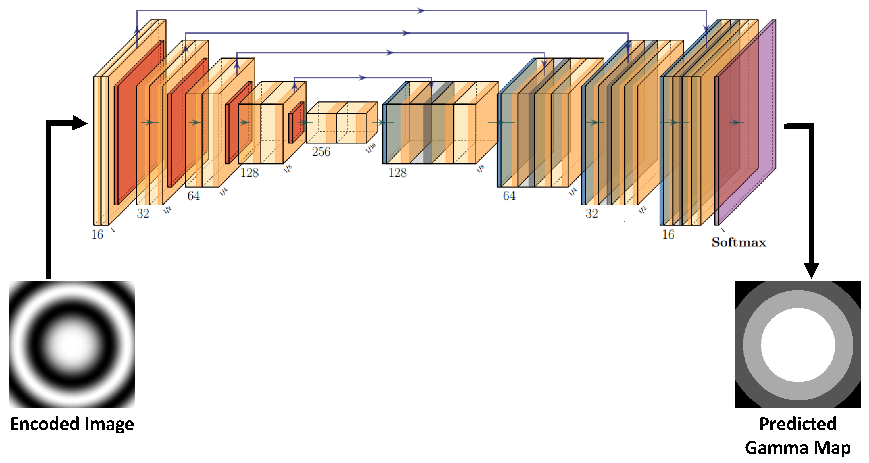
2.4. Single-Channel Depth Decoding with Semantic Segmentation

The method proposed in this section enables the recovery of depth information from a single-channel depth encoding using a semantic segmentation approach. This is accomplished by first calculating the unsigned wrapped phase from a single sinusoidal encoding in the same fashion as that demonstrated in [14]. This process can be described for each pixel $(i,j)$ as

$$\left|\varphi (i,j)\right|={cos}^{-1}(2I(i,j)-1).$$

(10)

However, this unsigned wrapped phase is inherently ambiguous, as each distinct grayscale value within the recovered $\left|\varphi \right|$ can represent any one of $2n$ depth values in the original geometry’s depth range (where n is the number of periods used in the encoding process). This ambiguity can be reduced by first associating a sign with every pixel of $\left|\varphi \right|$ via

$$\varphi (i,j)=\left\{\begin{array}{cc}+\mid \varphi (i,j)\mid \hfill & ,\gamma (i,j)\mathrm{is}\mathrm{even}\hfill \\ -\mid \varphi (i,j)\mid \hfill & ,\gamma (i,j)\mathrm{is}\mathrm{odd},\hfill \end{array}\right.$$

(11)

where the $\gamma$ is a gamma map that, for each pixel $(i,j)$, specifies whether the magnitude of the cosine encoding is increasing or decreasing. The generation of the gamma map is crucial and will be discussed later in this section. The resultant signed wrapped phase ($\varphi$) is conventionally referred to as only the wrapped phase.

Although this wrapped phase has less ambiguity than its unsigned counterpart, sharp discontinuities are present in $\varphi$ that must be resolved. These discontinuities occur at multiples of $2\pi$ within the total range of the original phase information, resulting in a total number of discontinuous phase regions equal to the number of encoding periods plus one ($n+1$). These sharp discontinuities can be removed through the use of a stair image, K, which determines the fringe order, or the number of $2\pi$ to add to each pixel of the wrapped phase, $\varphi$. This stair image can be calculated using the gamma map, $\gamma$, as

$$K(i,j)=\mathrm{Floor}\left(\frac{\gamma (i,j)}{2}\right).$$

(12)

A continuous absolute phase can be generated from K and $\varphi$ via

$$\mathsf{\Phi }(i,j)=\varphi (i,j)+2\pi \times K(i,j).$$

(13)

This absolute phase can then be scaled into the original depth dimensions of Z by

$$Z^{\prime }(i,j)=\frac{\mathsf{\Phi }(i,j)\times P}{2\pi }.$$

(14)

Thus far, this section has illustrated the necessity of the gamma map, $\gamma$, in the decoding of 3D-range data from a single sinusoidal encoding. An ideal gamma map can be computed from the original depth information, Z, as

$${\gamma }_{Ideal}(i,j)=\mathrm{Floor}\left(2\times \frac{Z(i,j)-\mathrm{Min}\left(Z\right)}{P}\right).$$

(15)

However, knowledge of the original depth information is, of course, unavailable at the time of decoding. This section proposes the use of a deep-learning algorithm in order to generate an in-situ gamma map through the semantic segmentation of the 8-bit encoded image, I. This is possible because the number of labeled regions within $\gamma$ that must be determined is fixed based on the number of periods (n) used to generate the encoded image, I. Additionally, the labels associated with each pixel of $\gamma$ are dependent on the structure of the data being encoded, which is often very similar across the range of 3D scans that a specific application may require to be compressed.

A U-Net architecture [21] was chosen to accomplish this gamma segmentation task due to the simplicity of its implementation and its ability to achieve high segmentation accuracy on smooth images. The specific architecture implemented is illustrated in Figure 1. This U-Net implementation has encoding blocks (shown on the left half of Figure 1) comprised of $3\times 3$ convolutions using the LeakyReLU activation function, with batch normalization, followed by $2\times 2$ maximum pooling layers. Each block of the encoder reduces the size of the feature layers by half while doubling the total number of layers. For this semantic segmentation problem, a maximum of 256 feature layers was chosen; increasing this number did not substantially improve performance. The decoding blocks used (shown on the right half of Figure 1) increase the size of the feature layers by two while reducing the number of layers by one half. Following this process, the outputs from each block of the decoder are concatenated with the equivalent-sized encoder block outputs (i.e., skip connections). These concatenated outputs are then passed through the same $3\times 3$ convolution operations used in the encoder. It should be noted that the number of $3\times 3$ convolutions applied in each block of the encoder and decoder are equal to the number of classes it is necessary to segment. For the example data shown in Figure 1, the number of classes is four, which means that four $3\times 3$ convolutions are applied for every block. The output of the final decoder block is then passed through the Softmax activation function, which allows for the determination of a probability distribution over the number of segmentation classes [22]. As illustrated in Figure 1, a trained implementation of this model allows an 8-bit encoded image to be input into the network, resulting in a predicted gamma map, $\gamma$, at the output. Model training is performed using pairs of encoded images (defined in Equation (9)) and their corresponding ideal gamma maps (defined in Equation (15)). Further training details, and experimental results, will be given for specific datasets in Section 3.

This novel method for the recovery of compressed 3D-range data from a single 8-bit grayscale encoded image, using deep-learning segmentation techniques, is illustrated in Figure 2. Figure 2a is a 3D rendering of the original data to be compressed. Figure 2b is Z, the 2D depth map corresponding to the original 3D data. In this case, Z is a $256\times 256$ ideal Gaussian surface with a depth range of 100 mm. Figure 2c is I, the sinusoidally encoded depth information generated using Equation (9), stored in the PNG image format. Figure 2d is the ideal gamma map, ${\gamma }_{Ideal}$, calculated from Z using Equation (15). Figure 2e is the unsigned wrapped phase, $\left|\varphi \right|$, decoded from Figure 2c using Equation (10). Figure 2f is the gamma map, $\gamma$, predicted from only Figure 2c using the trained U-Net architecture illustrated in Figure 1. Figure 2g is the wrapped phase, $\varphi$, where the sign of each pixel is determined using $\gamma$ (Figure 2f) according to Equation (11). Figure 2h is a 3D rendering of $Z^{\prime }$, the depth information recovered from $\varphi$ using $\gamma$ according to Equations (12)–(14).

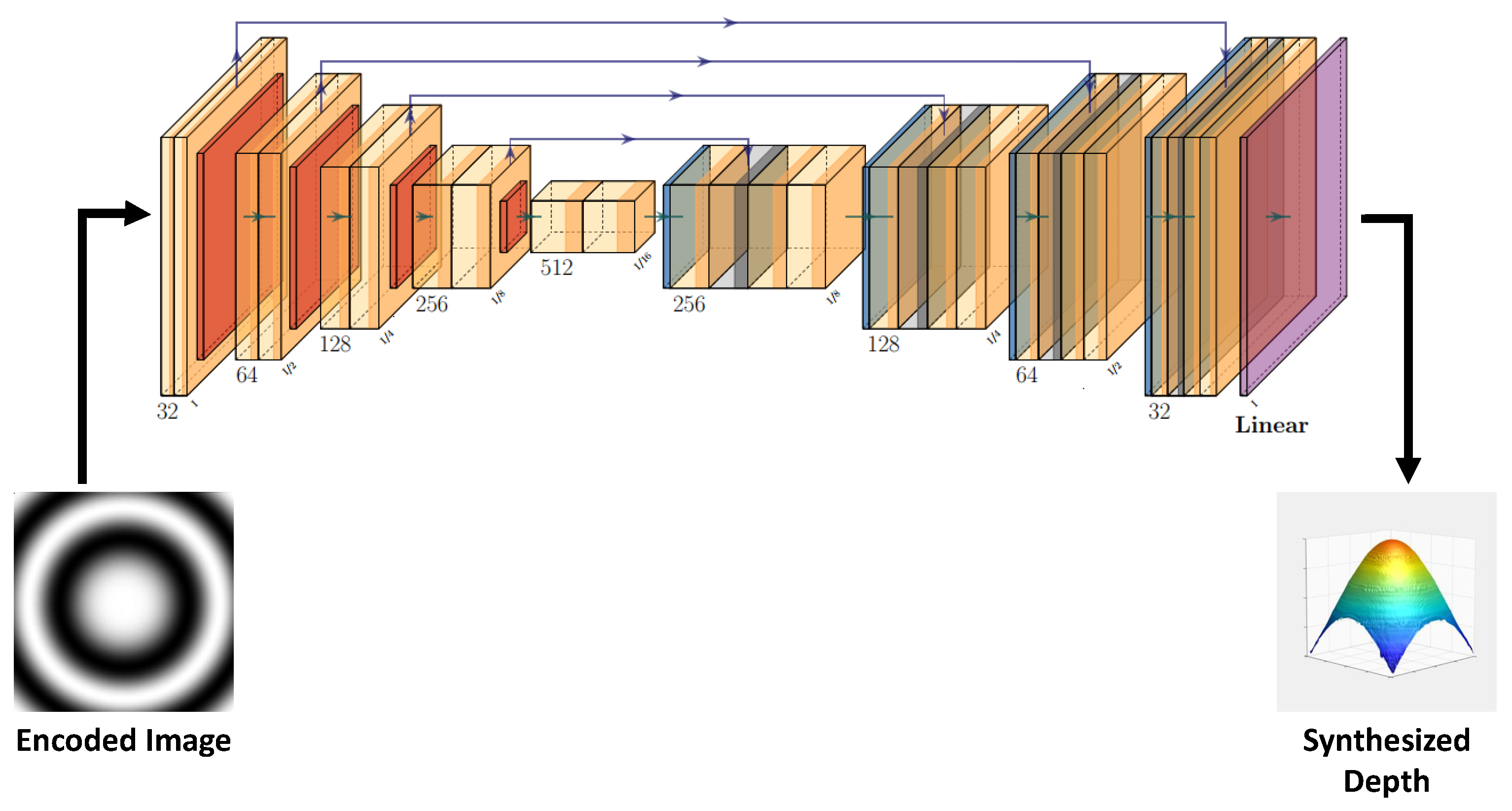
2.5. Single-Channel Depth Decoding with End-to-End Synthesis of Depth

Although the segmentation task discussed in the previous section is capable of recovering depth information from only a single-channel 8-bit image, artifacts may occur where $\gamma$ is incorrectly segmented from the encoding. These artifacts often manifest as rings occurring at fixed intervals throughout the depth range, corresponding to the boundaries between the different labels associated with the gamma map. Although these errors are often very small in magnitude, they can result in surfaces that lack the subjective visual fidelity required for some applications. Thus, this section proposes a different method for the recovery of depth information from a single-channel encoding. In this case, the 3D information is recovered through the use of a deep-learning model that enables end-to-end depth synthesis.

The architecture chosen to accomplish this synthesis task is a similar U-Net [21] to the one described in Section 2.4, with some modifications. This implementation is illustrated in Figure 3. The encoding blocks (shown on the left half of Figure 3) use the same $3\times 3$ convolutions with batch normalization and LeakyReLU, while $2\times 2$ maximum pooling layers are again used to reduce the size of the feature layers by one half while doubling the total number of layers at each block. This synthesis model used a maximum of 512 feature layers in order to reconstruct depth information from the encoded input data. The decoding blocks used (shown on the right half of Figure 3) invert the max pooling operation used in the encoder; feature layers are doubled in size while reducing the overall number of layers by one half. The outputs of this inverse pooling are concatenated with their equivalent-sized feature maps from the encoder and then passed through the same $3\times 3$ convolutions as used previously. Since this is a synthesis task, the number of convolutions performed in each block of the encoder and decoder is only one, unlike in the segmentation task described in Section 2.4. The output of the last decoder block is passed through the Linear activation function, which simply passes all values through, unmodified. Figure 3 illustrates that this model, once trained, allows for 8-bit encoded grayscale images to be input to the network with synthesized depth information ($Z_{Predicted}$) being recovered from the network’s output. Model training for this task is performed with pairs consisting of encoded images (defined in Equation (9)) and their corresponding ground-truth depth maps. Further training details, and experimental results, will be given for the specific datasets being analyzed in Section 3.

3. Experimental Results

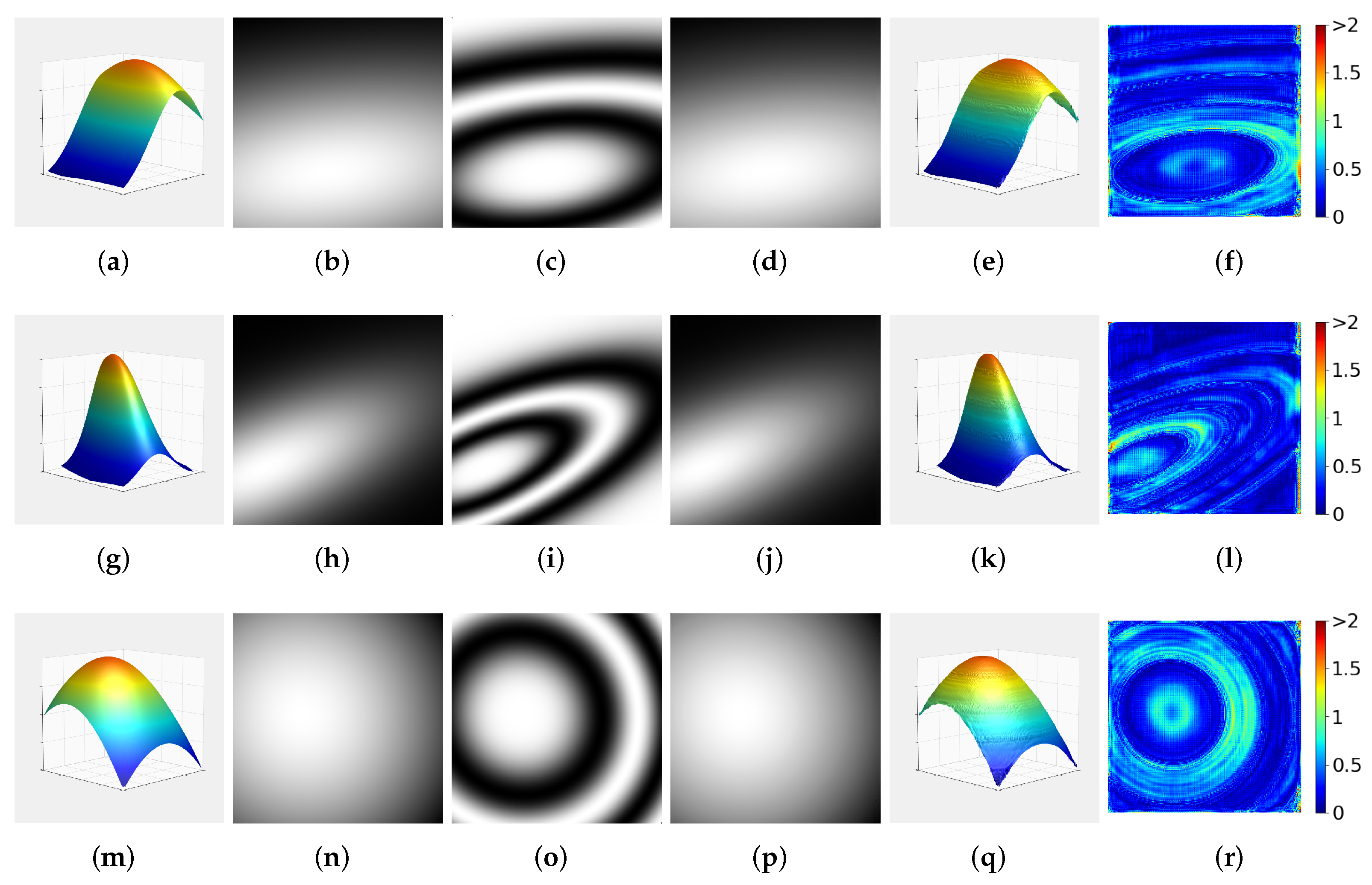
3.1. Random Gaussian Surfaces

The first dataset used to train and evaluate the proposed methods for decoding depth information from a single 8-bit grayscale image was a set of 1000 random Gaussian surfaces. Random values for $\sigma$ and $\mu$ were used to generate these surfaces, although these parameters were constrained such that the resulting surface would fill the majority of the $256\times 256$ image dimensions (i.e., each surface would not be near-zero for most of the image space). The depth range of these surfaces was normalized between zero and 100 mm. In their raw, floating-point format, each surface has an associated file size of 256 KB ($256\times 256\times 4$ bytes). These Gaussian surfaces were then sinusoidally encoded according to Equation (9) with $n=2$. This dataset was split into 80%, 10%, 10% subsets used for training, validation, and testing, respectively. The results reported in this section use only the testing subset, which was kept independent of the model during the training process. All models evaluated in this manuscript were trained using TensorFlow [23], a Python library developed for machine learning.

The first decoding approach evaluated on this dataset is the semantic segmentation for phase unwrapping discussed in Section 2.4. For simplicity, this approach to decoding is referred to as segmentation. The training for this model was conducted using the proposed grayscale encoded images as input, stored in the PNG format. Each encoding’s ideal gamma map, defined in Equation (15), was used as the ground-truth segmentation result. It should be noted that four distinct labeled regions exist within these ideal gamma maps. The loss function used for training was sparse categorical cross-entropy, and the Adam optimizer was selected with a fixed learning rate of ${10}^{-4}$. This model was trained for 100 epochs, with a batch size of 16, while monitoring validation accuracy. The model weights were saved for every epoch with the highest validation accuracy; in this case, epoch 99 was selected with an associated validation accuracy of 99.7%.

Figure 4 illustrates the proposed method of depth decoding utilizing semantic segmentation techniques. The three rows correspond to the first three random surfaces drawn from the testing subset. Column one shows a 3D rendering of the original depth information, Z. Column two shows the sinusoidally encoded image (stored in the PNG image format) generated using Equation (9) with $n=2$. Column three illustrates the ideal gamma map generated using Equation (15). Column four gives the predicted gamma-maps output from the trained segmentation model when the encoded images from column two were used as inputs. Column five shows 3D renderings of $Z^{\prime }$, the depth information recovered using the encoded image and the predicted gamma map using Equations (10)–(14) via the procedure described in Section 2.4. The sixth column shows the absolute error, in mm, between the recovered depth information ($Z^{\prime }$) and the original floating-point depth information (Z).

Next, this dataset was used to evaluate the end-to-end depth synthesis approach discussed in Section 2.5. This method will be referred to in this section as synthesis, for convenience. The synthesis model was trained using the single-channel encoded image (stored in the PNG image format) as input, while the original floating-point depth information (Z) was used as the ground truth. The loss function evaluated in training was a custom root mean squared error (RMSE) function calculated between the predicted output ($Z_{Predicted}$) and ground truth, which can be defined mathematically as

$$RMSE=\sqrt{\frac{{\sum }_{i,j}{(Z-Z_{Predicted})}^2}{H\times W}},$$

(16)

where the summation occurs over each pixel of the squared error. The values for H and W are the image height and width, respectively. An Adam optimizer was selected for this task with a fixed learning rate of ${10}^{-4}$. The synthesis model was trained for 450 epochs, with a batch size of 4, while monitoring the validation loss. Model weights for each subsequent epoch with the best performance were saved. For this experiment, epoch 330 was selected with an associated validation loss of 0.99%.

Figure 5 illustrates the proposed synthesis method for the recovery of depth information from a single-channel grayscale encoding stored in the PNG format. Each row corresponds to the first three random surfaces in the testing subset. Column one shows a 3D rendering of the original depth information, Z. Column two shows the corresponding 2D depth map. Column three gives the sinusoidally encoded depth maps, generated using Equation (9), stored in the PNG format. Column four contains the synthesized 2D depth maps ($Z_{Predicted}$) output by the trained synthesis model when the encoded images from column three are used as inputs. Column five shows 3D renderings of the synthesized depth information from column four. The sixth column shows the absolute error (in mm) when the synthesized depth information is compared to the original floating-point depth data.

Table 1. Performance of the proposed methods when the random Gaussian-surface testing dataset was encoded and stored in the PNG format.

PNG	Original File Size (KB)	Mean File Size (KB)	Mean Compression Ratio	Mean RMSE (mm)	Mean RMS Reconstruction Accuracy
Segmentation	256	12.55	20:1	0.294	99.70%
Synthesis				0.539	99.46%

provides numerical results for the proposed segmentation and synthesis methods when the random Gaussian surface testing subset was analyzed. The average file size for the original floating-point surfaces is 256 KB. This file size was reduced to an average of 12.55 KB when sinusoidally encoded and stored in a single 8-bit PNG image, achieving an average compression ratio of 20:1 for both proposed methods. It can also be seen that both of the proposed methods were able to achieve well above 99% reconstruction accuracies, which is suitable for many applications.

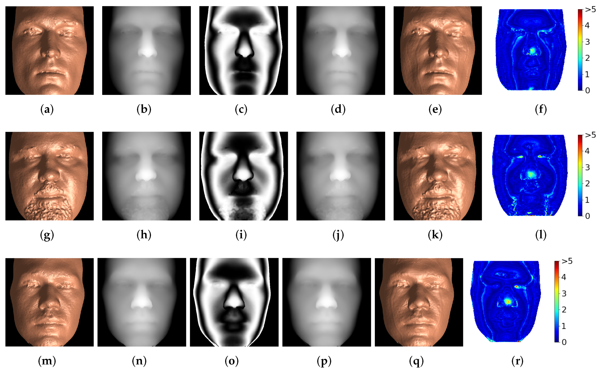
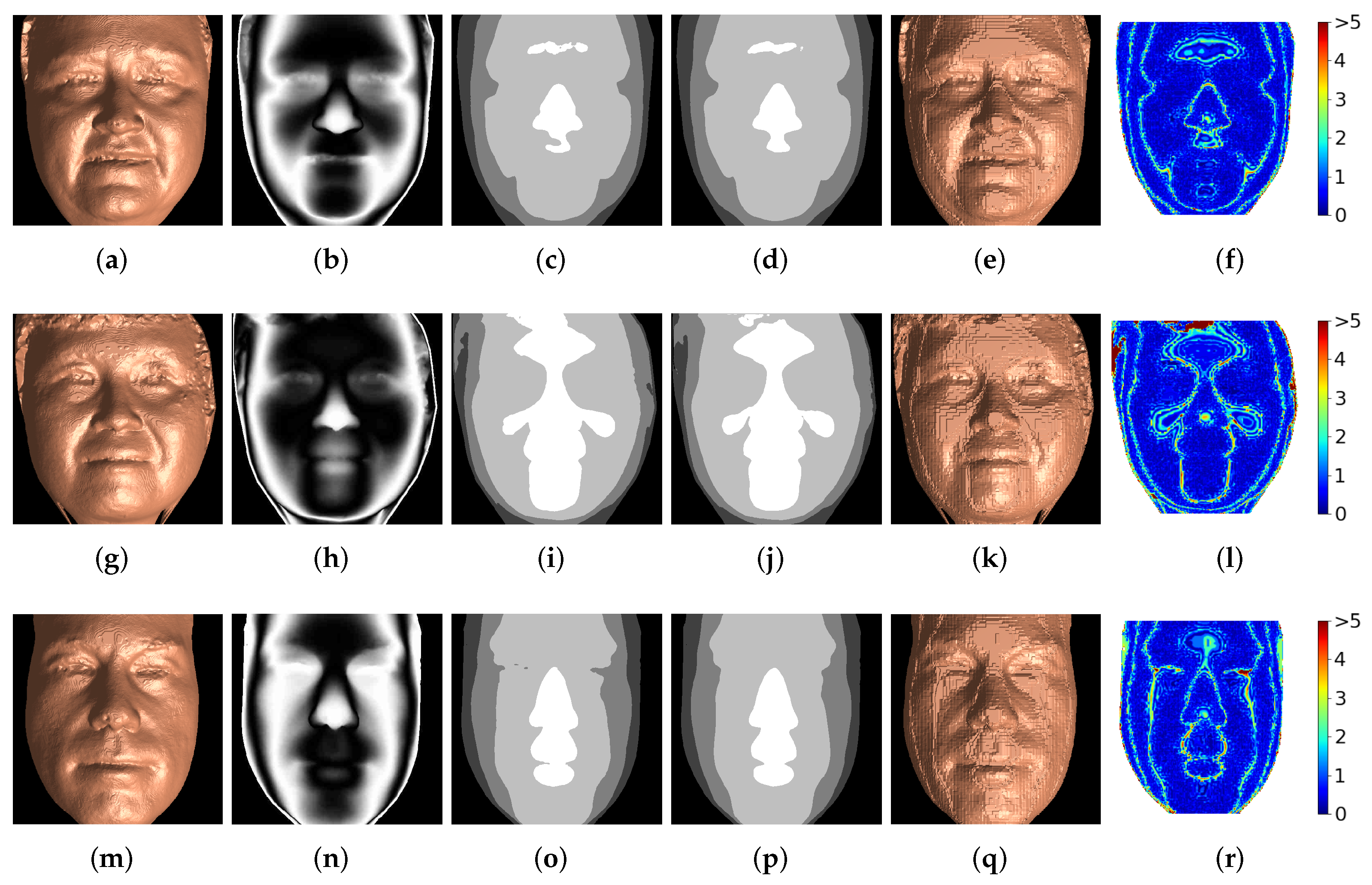
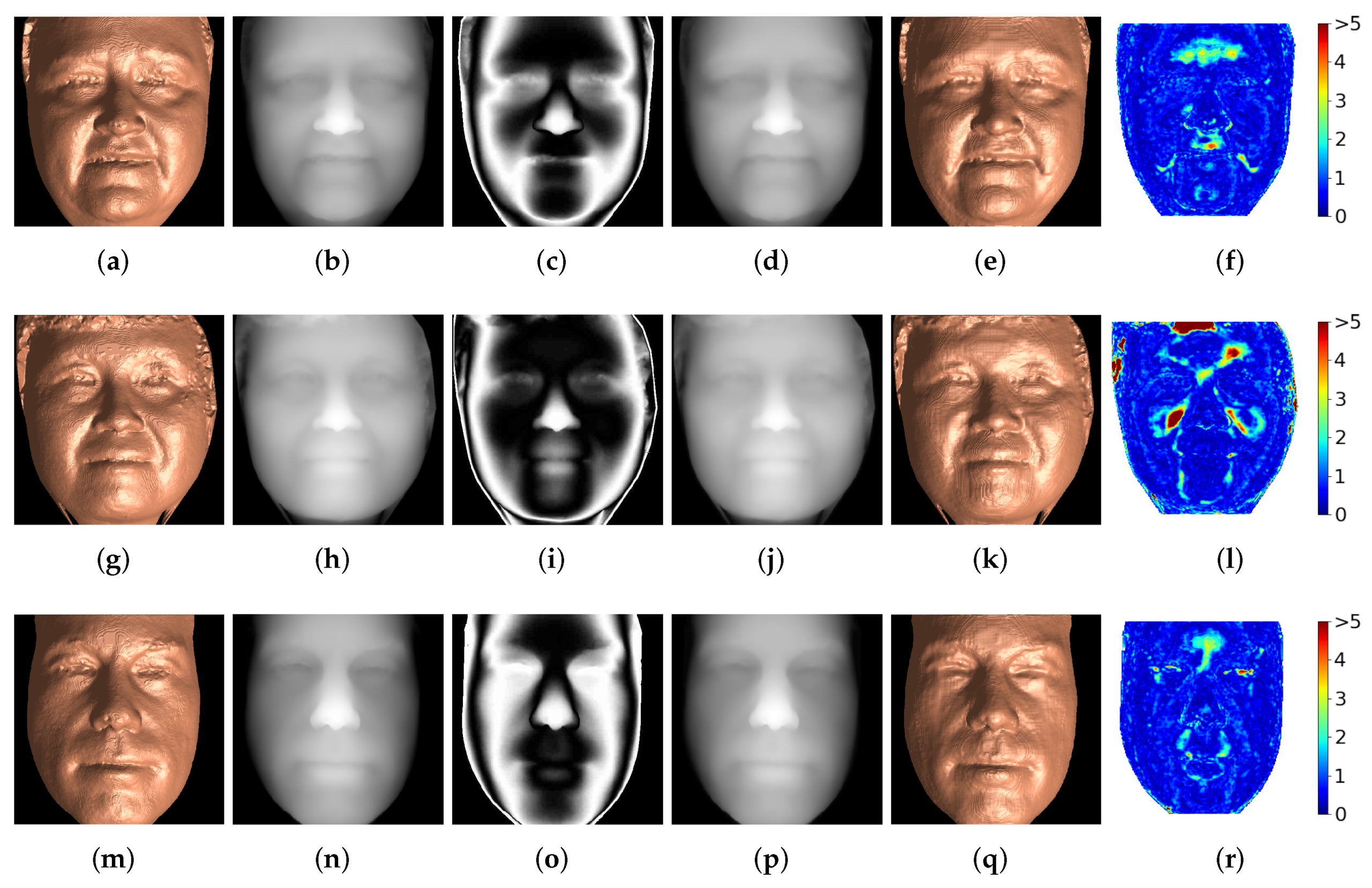
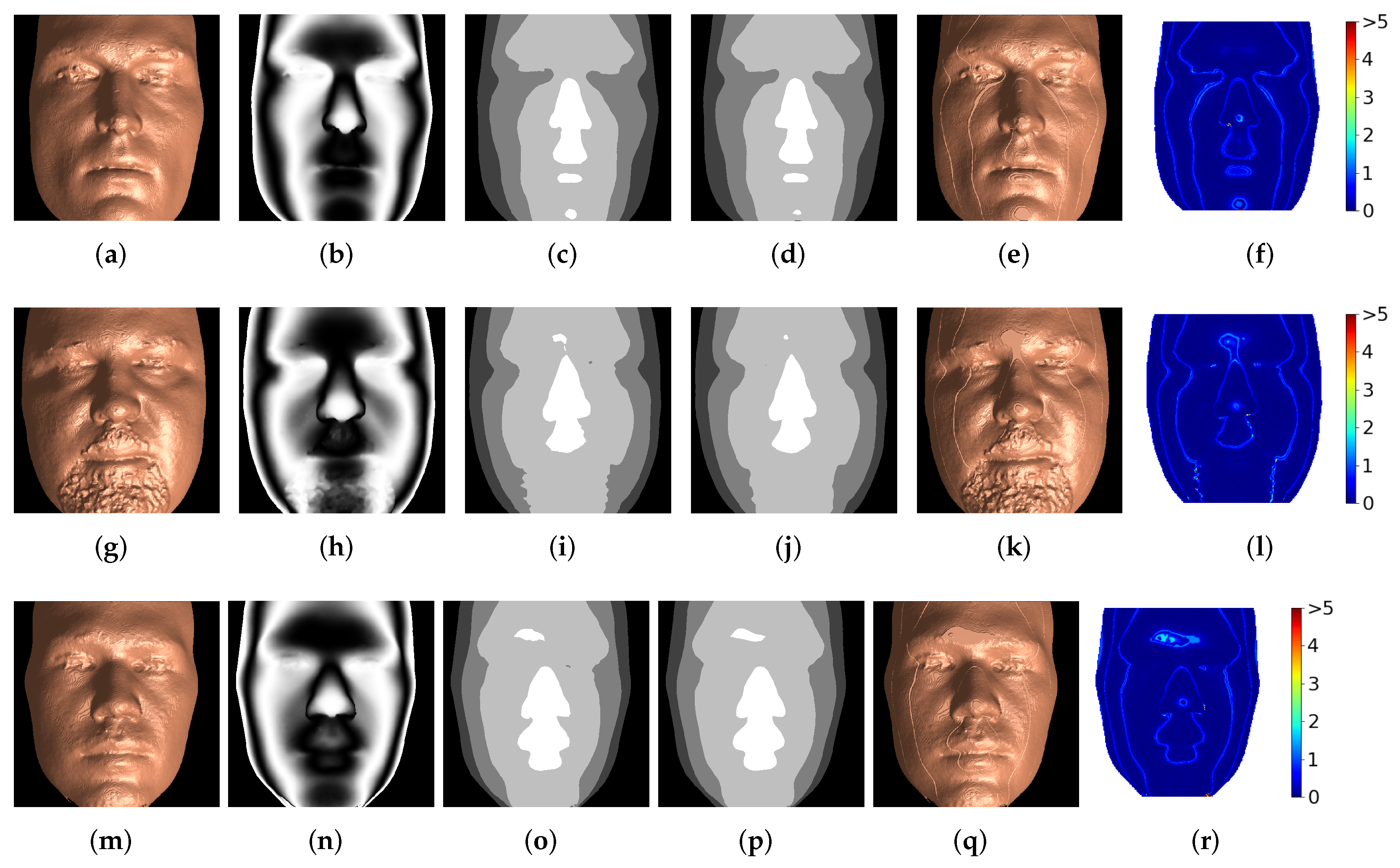
3.2. Texas 3D Face Recognition Database

To evaluate the proposed methods with geometry that is more complex, a second set of experiments was performed. The dataset selected was one that is representative of the type of data commonly used in applications such as telepresence and security (e.g., facial recognition). Here, 3D scans of human faces from the University of Texas’ 3D Facial Recognition Database [24,25,26] were cropped and zero-padded to dimensions of $512\times 512$ pixels. These depth maps, once cropped and padded into the expected dimensions, were passed through a 2D Gaussian filter with $\sigma =0.5$ and normalized between zero and 255 mm in order to ensure the depth values were floating-point. These raw, floating-point scans have an associated file size of 1024 KB ($512\times 512\times 4$ bytes). Each depth map was encoded using Equation (9) with two encoding periods (i.e., $n=2$). These 1149 scans were randomly shuffled and split into subsets with lengths 800, 100, and 149 for training, validation, and testing, respectively. The results reported are the results of analysis on only the testing subset, which was kept independent of the model during the training process.

The first decoding method evaluated on this dataset is the segmentation approach discussed in Section 2.4. Each encoded image in the dataset was paired with its corresponding ideal gamma map, ${\gamma }_{Ideal}$, generated using Equation (15). It should be noted that the original scans have an associated background that is unrelated to the faces themselves; as a result, these ideal gamma maps were generated with an additional integer value (in this case, zero) corresponding to the background pixels. Thus, this segmentation task aims to apply five labels to the resulting output gamma map, unlike the four labels required for the random Gaussian surfaces. The training for this segmentation model is identical to the training scheme utilized for the segmentation of the random Gaussian surface dataset: an Adam optimizer with a fixed learning rate of ${10}^{-4}$ was applied for 100 epochs while monitoring validation accuracy; the loss function used was sparse categorical cross-entropy; and the epoch selected, based on best validation accuracy, was epoch 86 with an associated validation accuracy of 99.20%.

The segmentation approach to the decoding of depth information from a grayscale image is shown for the first three scans in the testing subset in Figure 6. The first column shows 3D renderings of the original depth information, Z. The second column shows the sinusoidally encoded images generated using Equation (9) with two encoding periods, stored in the PNG format. The third column shows the ideal gamma map, ${\gamma }_{Ideal}$, generated using Equation (15). The fourth column shows the predicted gamma map generated by passing the encoded images from column two into the trained segmentation model discussed previously. Column five shows the reconstructed depth information, $Z^{\prime }$, calculated using the predicted gamma map and Equation (10)–(14) via the procedure described in Section 2.4. Finally, column six shows the absolute error when the reconstructed geometry is compared to the original, floating-point data.

Next, the synthesis approach to the recovery of depth information discussed in Section 2.5 was evaluated using this dataset. Here, each encoded image in the dataset was paired with its corresponding original floating-point depth map (Z). The training for this model is the same as the scheme utilized when training for the random Gaussian surface dataset: an Adam optimizer was utilized with a fixed learning rate of ${10}^{-4}$; the batch size used was four; and a custom RMSE loss function was monitored for the 450 epochs that the model was trained. The model weights were selected (based on best results from the validation subset) from epoch 273, with an associated validation loss of 0.61%. It should be noted that, since the depth information also contains irrelevant background pixels, the RMSE loss function that was minimized when training the synthesis model does not consider background pixels in its calculation.

The synthesis approach to the recovery of depth information from an 8-bit grayscale image is shown for the first three scans in the testing dataset in Figure 7. The first column shows a 3D rendering of the original floating-point depth information, Z. The second column shows the 2D depth map corresponding to the 3D renderings shown in the first column. Column three is the sinusoidally encoded depth image (with $n=2$) from column two, stored in the PNG image format. Column four is the output of the synthesis model, $Z_{Predicted}$, when the encoded image from the third column is input. The fifth column is a 3D rendering of the synthesized depth information shown in column four. Finally, column six is the absolute error when the recovered geometry is compared to the original, floating-point depth information.

The next experiment demonstrates the ability of the proposed segmentation method to recover depth information from a single-channel image when lossy compression is applied. In this case, the JPG image format was used to store the encoded output image, with the quality set to 20. The segmentation model was retrained with these JPG-20 encoded images using the same procedure described for the previously discussed case when PNG was used to store the output. Here, the model weights were selected from training epoch 73 with an associated validation accuracy of 99.0%. Figure 8 illustrates the proposed segmentation process on lossy encoded images for the first three faces from the testing subset, and each column directly corresponds to its equivalent column from Figure 6. Column one shows 3D renderings of the original depth information, Z. Column two shows the sinusoidally encoded images generated using Equation (9), stored in the JPG-20 image format. Column three and four are the ideal gamma maps and gamma maps predicted by the trained segmentation model, respectively. The recovered depth information is rendered in column five, and column six gives the absolute error for this reconstruction when compared to the original floating-point depth information. Note that, since the encoded images needed to be regenerated and stored in the JPG format, the random shuffling caused the training, validation, and testing subsets to differ from the lossless case discussed previously. Thus, the faces shown in Figure 8 are not the same as the faces shown in Figure 6.

Next, the synthesis approach was analyzed on the lossy encoded images. The synthesis model was retrained using the JPG 20 encoded images, following the same procedure as when the PNG encoded images were used. The model weights selected were generated at training epoch 353, with an associated validation loss of 0.51%. Figure 9 shows the experimental results for the proposed method of depth synthesis from lossy encoded images for the first three faces from the testing subset, and each column directly corresponds to its equivalent column from Figure 7. Columns one and two show the 3D renderings of the original depth information and the corresponding 2D depth maps, respectively. Column three shows the sinusoidally encoded depth maps from column two, generated using Equation (9), stored in the JPG 20 image format. Columns four and five respectively illustrate the synthesized 2D depth maps and corresponding 3D renderings output by the trained synthesis model when the encodings from the third column were input. The sixth column illustrates the absolute error for the synthesized depth maps compared to the original floating-point depth information.

Table 2. Performance of the proposed methods when the Texas Facial Recognition Database testing subset was encoded. (a) Average results for the proposed methods when the PNG image compression standard was used to store the single-channel encoding; (b) Average results for the proposed methods when the JPG image compression standard, with quality set to 20, was used to store the single-channel encoding.

(a)
PNG	Original File Size (KB)	Mean File Size (KB)	Mean Compression Ratio	Mean RMSE (mm)	Mean RMS Reconstruction Accuracy
Segmentation	1024	65.46	15:1	1.182	99.53%
Synthesis				0.996	99.60%
(b)
JPG 20	Original File Size (KB)	Mean File Size (KB)	Mean Compression Ratio	Mean RMSE (mm)	Mean RMS Reconstruction Accuracy
Segmentation	1024	9.65	106:1	2.066	99.18%
Synthesis				1.031	99.59%

provides numerical results for the total testing subset used in the evaluation of both the segmentation and synthesis approaches. Table 2a compares the mean aggregate file size and RMS depth recovery error for both approaches when the PNG image compression standard was applied to the encoded output image. Table 2b compares the mean aggregate file size and RMS depth recovery error for both approaches when the JPG 20 image compression standard was applied to the encoded output image. It should be noted that, for each individual image compression standard utilized (i.e., PNG and JPG 20), identical images were used as inputs to both models. As such, the mean file size and compression ratios are the same for each distinct image format. Additionally, the original floating-point data for this dataset will always have the same file size ($512\times 512\times 4$ bytes). It can be seen that both methods were able to achieve accuracies higher than 99%, regardless of the image compression format applied to the encoded output. Further, file sizes were significantly reduced: when the JPG-20 image format was used, a compression ratio of 106:1 was achieved when compared to the 1024 KB original data. These results illustrate that there was not a significant difference in reconstruction accuracy between encodings stored with lossless and lossy compression when the synthesis model was used. This may imply that the synthesis model learns to mitigate compression artifacts as it reconstructs depth data from lossy encodings. That said, one should note that this ability is not learned by the segmentation model. For instance, when the segmentation model was used with lossy JPG 20, as opposed to lossless PNG, there was a drastic increase in reconstruction error and a notable reduction in visual fidelity (as can be seen in Figure 8).

4. Discussion

The proposed methods of depth recovery from a single 8-bit sinusoidal encoding allow for high compression ratios to be achieved when compared to the original floating-point data. This was experimentally demonstrated in the previous section; both semantic image segmentation and end-to-end depth synthesis were utilized in the decoding of depth information from 8-bit grayscale images stored in lossless and lossy formats. However, several factors must be taken into account when evaluating the potential use-cases for these methods and when considering future research in this area. The following is a discussion of these factors.

• Generalizability.Section 3 illustrates the performance of both the segmentation and synthesis approaches to the recovery of depth information from a single-channel encoding. However, it is also important to evaluate the generalizability of the proposed methods to 3D-range scans from alternate datasets. This is demonstrated in Figure 10. Figure 10a is a 3D rendering of depth data from the University of York’s 3D Face Dataset [27]. In this case, the data is a 3D scan of a human face that has been cropped and reshaped to $512\times 512$ pixels in order to match the dimensions expected by the trained segmentation and synthesis models. Figure 10b is the corresponding 2D depth map, normalized between zero and 255 mm after removing unconnected components and being passed through a Gaussian filter ($\sigma =0.5$) in order to ensure floating-point precision. Figure 10c is the sinusoidally encoded depth map, generated according to Equation (9) and stored in the PNG image format. Figure 10d is a 3D rendering of the segmentation method’s output, trained using the Texas 3D Face Recognition Database [24,25,26], when the sinusoidal encoding in (c) is used as input. Figure 10e is a 3D rendering of the synthesis model’s output, trained using the Texas 3D Face Recognition Database [24,25,26], when the sinusoidal encoding in (c) is used as input. It can be seen that the depth recovered by both segmentation and synthesis are reasonably faithful to the original 3D-range data, especially when artifacts near the surface edges are ignored. This shows that the segmentation and synthesis models are reasonably generalizable to similar data from alternate datasets; however, it was necessary to carefully crop this alternate input in order to match the approximate structure and alignment of the data used to train the models. It is important to note that, while these models may perform adequately for one particular type of data, they do not necessarily have the ability to generalize and perform well on any given encoding of 3D-range data. For instance, all results presented thus far have shown that depth data can be recovered from the segmentation and synthesis models trained with encodings of a particular class of depth data: Gaussian random surfaces were recovered from their encodings with models trained on encodings of Gaussian random surfaces, and 3D faces were recovered from their encodings with models trained on encodings of 3D faces. If the Gaussian-trained models were tasked with recovering depth from encodings of 3D faces, for example, they may have trouble as deformations in the encodings caused by facial structures (i.e., eyes, noses, mouths) were not seen within the training data. Figure 10f,g show the models’ limited ability to generalize outside of its training set. In these examples, an encoding of the face data in Figure 10a was decoded using the segmentation and synthesis models trained on random Gaussian surfaces. It is clear that both approaches fail to reconstruct the proper shape of the face. This is expected, as each Gaussian-trained model (segmentation and synthesis) was never provided information on how to reconstruct facial encodings (i.e., they only know how to aid in recovering the depth of Gaussian surface encodings). Further, this indicates that each model is not simply learning how to perform an operation analogous to phase unwrapping, but that the models are learning and relying on the underlying structure of the 3D shape represented within the encodings. One naturally imagines a sophisticated model that can successfully recover depth of facial encodings, random Gaussian encodings, and surfaces in between. Achieving this level of broad generalizability is challenging; however, useful avenues of future work to help ensure that trained models are more generalizable include: (1) training with more robust datasets that contain various subject categories with both single continuous and multiple disjoint surfaces; (2) data augmentation; and (3) automated dataset generation via virtual environments [20].
• Encoding Frequency. Throughout this manuscript, depth information was successfully recovered—with a high degree of accuracy—from within 8-bit grayscale images. However, the performance of the proposed segmentation and synthesis methods was only evaluated for a relatively low depth range and number of encoding periods ($n=2$). It is important to note that, as the number of encoding periods increases, the complexity of the problem that must be solved by the segmentation approach also increases. This is because the number of regions that must be correctly segmented and labeled in order to generate the gamma map, $\gamma$, increases proportionally to the number of encoding periods. This proportional increase in segmentation complexity will result in a higher rate of error and a subsequent loss in subjective visual fidelity, particularly at segmentation boundaries. Liang et al. proposed a method that mitigates this problem of increased semantic segmentation complexity associated with a higher number of encoding periods for phase unwrapping in DFP systems [28]. This was performed through the use of two deep-learning networks in series. The first network generates a segmented and labeled image associated with the features of the captured fringes; the second network uses this semantic segmentation as input and outputs correctly unwrapped phase images. Similar techniques could potentially be applied to phase unwrapping for the 3D-range geometry compression of either multiple disjoint or single continuous surfaces, although the authors of this manuscript leave it as an avenue for future work.
• Error Correction. The numerical performance of the segmentation and synthesis approaches discussed in this manuscript are nearly identical when a lossless image format such as PNG is used to store the encoded output. However, the segmentation approach has reconstruction error that, in general, manifests as rigid, ring-like artifacts that occur at boundaries between the labeled regions segmented by the model. The synthesis approach has an error that occurs with less structure, and is more evenly distributed throughout the 3D scene. One method of potentially reducing the impact of the segmentation errors on subjective visual fidelity is to perform error correction using the output of both the segmentation and synthesis models. For example, an edge-detection algorithm could be applied to the gamma map generated by the segmentation approach; this would correspond to regions of assumed error, since most of the segmentation error is associated with these boundaries. Next, the depth information decoded using the segmentation approach could have its regions of assumed error replaced with the corresponding pixels from the synthesized depth information. Finley and Bell experimentally demonstrated a conceptually similar method of error correction using heavily filtered data to replace regions of assumed error [14]. Additionally, deep-learning techniques have been recently applied to the classification and correction of errors in 3D representations [29] and are an exciting future avenue for potential error-correction frameworks.
• Potential Applications. This manuscript illustrated two novel methods for the recovery of floating-point depth information from only a single 8-bit image channel. Both of these methods utilize deep-learning techniques in order to decode the depth information and are able to achieve above 99% RMS reconstruction accuracy even when the depth encoding is stored in the JPG-20 image format. This allows for very large compression ratios to be achieved when compared to the original floating-point depth information. However, since these two methods of 3D-range geometry compression are enabled through the use of deep-learning networks, they are constrained to use cases where a large quantity of similarly structured depth data is available for training. Additionally, since the priority of these compression methods is small file sizes instead of high fidelity, they are potentially suitable for applications where some small degree of measurement error or reduction in visual fidelity can be tolerated. Some example applications that typically meet these requirements are real-time 3D telepresence and 3D facial recognition. However, the ethical ramifications of potential misrepresentation due to decoding errors must also be considered when applying deep-learning techniques to applications such as facial recognition. Given the potential uncertainty and abstract nature of the results produced by deep-learning models, it is often challenging to determine—from the output data alone—how representative of the original data the output may be.

5. Conclusions

This manuscript has presented two novel methods for the compression and subsequent recovery of 3D-range data from a single 8-bit grayscale encoded image using deep-learning techniques. Specifically, semantic image-segmentation techniques and end-to-end depth synthesis were utilized in order to reduce the file sizes associated with the storage of depth information. The proposed methods are compatible with both lossless and lossy image compression formats, allowing for very high compression ratios to be achieved when compared to the original floating-point depth data. For example, when complex 3D scans of human faces were encoded and stored in the JPG-20 image format, an average compression ratio of 106:1 was achieved. Further, both methods of recovering depth information from a single-channel encoded image are capable of achieving reconstruction accuracies suitable for many applications. When the JPG-20 image format was used to store the encoded output, the segmentation approach achieved a mean RMS reconstruction accuracy of 99.18% while the synthesis approach was capable of generating surfaces with an accuracy of 99.59%. This manuscript also provided discussion of the generalizability of the machine-learning models used, highlighted a potential method of error correction for incorrectly segmented data, and discussed several avenues of potential future work.

References

1. Zhang, S. High-speed 3D shape measurement with structured light methods: A review. Opt. Lasers Eng. 2018, 106, 119–131. [Google Scholar] [CrossRef]
2. Maglo, A.; Lavoué, G.; Dupont, F.; Hudelot, C. 3D Mesh Compression: Survey, Comparisons, and Emerging Trends. ACM Comput. Surv. 2015, 47, 1–41. [Google Scholar] [CrossRef]
3. Orts-Escolano, S.; Rhemann, C.; Fanello, S.; Chang, W.; Kowdle, A.; Degtyarev, Y.; Kim, D.; Davidson, P.L.; Khamis, S.; Dou, M.; et al. Holoportation: Virtual 3d teleportation in real-time. In Proceedings of the 29th Annual Symposium on User Interface Software and Technology, Tokyo, Japan, 16–19 October 2016; pp. 741–754. [Google Scholar]
4. Guo, K.; Lincoln, P.; Davidson, P.; Busch, J.; Yu, X.; Whalen, M.; Harvey, G.; Orts-Escolano, S.; Pandey, R.; Dourgarian, J.; et al. The relightables: Volumetric performance capture of humans with realistic relighting. ACM Trans. Graph. TOG 2019, 38, 1–19. [Google Scholar] [CrossRef] [Green Version]
5. Gu, X.; Gortler, S.J.; Hoppe, H. Geometry images. In Proceedings of the 29th Annual Conference on Computer Graphics and Interactive Techniques, San Antonio, TX, USA, 23–26 July 2002; pp. 355–361. [Google Scholar]
6. Gu, X.; Zhang, S.; Huang, P.; Zhang, L.; Yau, S.T.; Martin, R. Holoimages. In Proceedings of the 2006 ACM Symposium on Solid and Physical Modeling, Cardiff, UK, 6–8 June 2006; pp. 129–138. [Google Scholar]
7. Karpinsky, N.; Zhang, S. Composite phase-shifting algorithm for three-dimensional shape compression. Opt. Eng. 2010, 49, 063604. [Google Scholar] [CrossRef]
8. Zhang, S. Three-dimensional range data compression using computer graphics rendering pipeline. Appl. Opt. 2012, 51, 4058–4064. [Google Scholar] [CrossRef] [PubMed] [Green Version]
9. Ou, P.; Zhang, S. Natural method for three-dimensional range data compression. Appl. Opt. 2013, 52, 1857–1863. [Google Scholar] [CrossRef] [PubMed]
10. Bell, T.; Zhang, S. Multiwavelength depth encoding method for 3D range geometry compression. Appl. Opt. 2015, 54, 10684–10691. [Google Scholar] [CrossRef] [PubMed]
11. Hou, Z.; Su, X.; Zhang, Q. Virtual structured-light coding for three-dimensional shape data compression. Opt. Lasers Eng. 2012, 50, 844–849. [Google Scholar] [CrossRef]
12. Wang, Y.; Zhang, L.; Yang, S.; Ji, F. Two-channel high-accuracy Holoimage technique for three-dimensional data compression. Opt. Lasers Eng. 2016, 85, 48–52. [Google Scholar] [CrossRef]
13. Bell, T.; Vlahov, B.; Allebach, J.P.; Zhang, S. Three-dimensional range geometry compression via phase encoding. Appl. Opt. 2017, 56, 9285–9292. [Google Scholar] [CrossRef] [PubMed]
14. Finley, M.G.; Bell, T. Two-channel depth encoding for 3D range geometry compression. Appl. Opt. 2019, 58, 6882–6890. [Google Scholar] [CrossRef] [PubMed]
15. Finley, M.G.; Bell, T. Two-channel 3D range geometry compression with primitive depth modification. Opt. Lasers Eng. 2022, 150, 106832. [Google Scholar] [CrossRef]
16. Li, B.; Karpinsky, N.; Zhang, S. Novel calibration method for structured-light system with an out-of-focus projector. Appl. Opt. 2014, 53, 3415–3426. [Google Scholar] [CrossRef] [PubMed]
17. Zhang, S. Absolute phase retrieval methods for digital fringe projection profilometry: A review. Opt. Lasers Eng. 2018, 107, 28–37. [Google Scholar] [CrossRef]
18. Yin, W.; Chen, Q.; Feng, S.; Tao, T.; Huang, L.; Trusiak, M.; Asundi, A.; Zuo, C. Temporal phase unwrapping using deep learning. Sci. Rep. 2019, 9, 20175. [Google Scholar] [CrossRef] [PubMed]
19. Qian, J.; Feng, S.; Tao, T.; Hu, Y.; Li, Y.; Chen, Q.; Zuo, C. Deep-learning-enabled geometric constraints and phase unwrapping for single-shot absolute 3D shape measurement. Apl Photonics 2020, 5, 046105. [Google Scholar] [CrossRef]
20. Zheng, Y.; Wang, S.; Li, Q.; Li, B. Fringe projection profilometry by conducting deep learning from its digital twin. Opt. Express 2020, 28, 36568–36583. [Google Scholar] [CrossRef] [PubMed]
21. Ronneberger, O.; Fischer, P.; Brox, T. U-net: Convolutional networks for biomedical image segmentation. In International Conference on Medical Image Computing and Computer-Assisted Intervention; Springer: Berlin/Heidelberg, Germany, 2015; pp. 234–241. [Google Scholar]
22. Goodfellow, I.; Bengio, Y.; Courville, A. Deep Learning; MIT Press: Cambridge, MA, USA, 2016. [Google Scholar]
23. Abadi, M.; Barham, P.; Chen, J.; Chen, Z.; Davis, A.; Dean, J.; Devin, M.; Ghemawat, S.; Irving, G.; Isard, M.; et al. Tensorflow: A system for large-scale machine learning. In 12th USENIX Symposium on Operating Systems Design and Implementation (OSDI 16); USENIX Association: Savannah, GA, USA, 2016; pp. 265–283. [Google Scholar]
24. Gupta, S.; Markey, M.K.; Bovik, A.C. Anthropometric 3D face recognition. Int. J. Comput. Vis. 2010, 90, 331–349. [Google Scholar] [CrossRef]
25. Gupta, S.; Castleman, K.R.; Markey, M.K.; Bovik, A.C. Texas 3D face recognition database. In Proceedings of the 2010 IEEE Southwest Symposium on Image Analysis & Interpretation (SSIAI), Austin, TX, USA, 23–25 May 2010; pp. 97–100. [Google Scholar]
26. Gupta, S.; Castleman, K.R.; Markey, M.K.; Bovik, A.C. Texas 3D Face Recognition Database. 2020. Available online: http://live.ece.utexas.edu/research/texas3dfr/index.htm (accessed on 27 June 2020).
27. Heseltine, T.; Pears, N.; Austin, J. Three-dimensional face recognition using combinations of surface feature map subspace components. Image Vis. Comput. 2008, 26, 382–396. [Google Scholar] [CrossRef]
28. Liang, J.; Zhang, J.; Shao, J.; Song, B.; Yao, B.; Liang, R. Deep convolutional neural network phase unwrapping for fringe projection 3d imaging. Sensors 2020, 20, 3691. [Google Scholar] [CrossRef] [PubMed]
29. Tanner, M.; Săftescu, S.; Bewley, A.; Newman, P. Meshed up: Learnt error correction in 3D reconstructions. In Proceedings of the 2018 IEEE International Conference on Robotics and Automation (ICRA), Brisbane, QLD, Australia, 21–25 May 2018; pp. 3201–3206. [Google Scholar]
Figure 1. The U-Net architecture employed for segmentation of gamma data from single-channel, 8-bit grayscale encoded images.
Photonics 09 00449 g001
Figure 2. The proposed single-channel encoding and decoding process applied to a smooth Gaussian surface. (a) 3D rendering of the original surface; (b) 2D depth map corresponding to the data in (a); (c) encoded image output by the proposed method, stored in the PNG format; (d) ground-truth gamma map calculated using the original data; (e) unsigned ϕ ; (f) gamma map predicted using semantic segmentation techniques; (g) signed ϕ , calculated using (e,f); (h) 3D rendering of the recovered geometry, calculated using (f,g).
Photonics 09 00449 g002
Figure 3. The U-Net architecture employed for end-to-end synthesis of depth data from single-channel, 8-bit grayscale encoded images.
Photonics 09 00449 g003
Figure 4. The proposed method of semantic image segmentation on random Gaussian surfaces when the 8-bit encoded images were stored in the PNG format. (Row 1)–(Row 3) correspond to the first three surfaces from the testing subset. (Column 1) 3D renderings of the original depth information with a depth range of 100 mm; (Column 2) Sinusoidal encodings of the original depth information, stored in the PNG format; (Column 3) Ideal gamma maps for the original depth information; (Column 4) Gamma maps predicted by passing the sinusoidal encodings into the trained segmentation model; (Column 5) 3D renderings of the depth information recovered using the predicted gamma maps and sinusoidal encodings; (Column 6) Absolute error (in mm) between the recovered depth information and original floating-point depth data.
Photonics 09 00449 g004
Figure 5. The proposed method of end-to-end depth synthesis on random Gaussian surfaces when the 256 × 256 encoded images were stored in the PNG format. (Row 1)–(Row 3) correspond to the first three surfaces from the testing subset. (Column 1) 3D renderings of the original depth information; (Column 2) 2D depth maps with a depth range of 100 mm; (Column 3) Sinusoidal encodings of the original depth information, stored in the PNG format; (Column 4) Depth maps recovered by passing the sinusoidal encodings through the trained synthesis model; (Column 5) 3D renderings of the synthesized depth maps; (Column 6) Absolute error (in mm) between the synthesized depth information and original floating-point depth data.
Photonics 09 00449 g005
Figure 6. Proposed method of semantic image segmentation on 3D scans of faces [24,25,26] when the 8-bit encoded images were stored with PNG. (Row 1)–(Row 3) are the first three scans from the testing subset. (Column 1) 3D renderings of the original depth data with a depth range of 255 mm; (Column 2) Sinusoidal encodings of the original depth data, stored in the PNG format; (Column 3) Ideal gamma maps for the original depth data; (Column 4) Gamma maps predicted by passing the sinusoidal encodings into the trained segmentation model; (Column 5) 3D renderings of the depth data recovered using the predicted gamma maps and sinusoidal encodings; (Column 6) Absolute error (in mm) between the recovered depth data and original floating-point depth data.
Photonics 09 00449 g006
Figure 7. The proposed method of end-to-end depth synthesis on 3D scans of human faces [24,25,26] when the 512 × 512 encoded images were stored in the PNG format. (Row 1)–(Row 3) correspond to the first three surfaces from the testing subset. (Column 1) 3D renderings of the original depth information; (Column 2) Depth maps with a depth range of 255 mm; (Column 3) Sinusoidal encodings of the original depth information, stored in the PNG format; (Column 4) 2D depth maps recovered by passing the sinusoidal encodings through the trained synthesis model; (Column 5) 3D renderings of the synthesized depth maps; (Column 6) Absolute error (in mm) between the synthesized depth information and original floating-point depth data.
Photonics 09 00449 g007
Figure 8. The proposed method of semantic image segmentation on 3D scans of human faces [24,25,26] when the 8-bit encoded images were stored in the JPG 20 format. (Row 1)–(Row 3) correspond to the first three scans from the testing subset. (Column 1) 3D renderings of the original depth information with a depth range of 255 mm; (Column 2) Sinusoidal encodings of the original depth information, stored in the JPG 20 format; (Column 3) Ideal gamma maps for the original depth information; (Column 4) Gamma maps predicted by passing the sinusoidal encodings into the trained segmentation model; (Column 5) 3D renderings of the depth information recovered using the predicted gamma maps and sinusoidal encodings; (Column 6) Absolute error (in mm) between the recovered depth information and original floating-point depth data.
Photonics 09 00449 g008
Figure 9. The proposed method of end-to-end depth synthesis on 3D scans of human faces [24,25,26] when the encoded images were stored in the JPG 20 format. (Row 1)–(Row 3) correspond to the first three surfaces from the testing subset. (Column 1) 3D renderings of the original depth information; (Column 2) 512 × 512 depth maps with a depth range of 255 mm; (Column 3) Sinusoidal encodings of the original depth information, stored in the JPG 20 format; (Column 4) 2D depth maps recovered by passing the sinusoidal encodings through the trained synthesis model; (Column 5) 3D renderings of the synthesized depth maps; (Column 6) Absolute error (in mm) between the synthesized depth information and original floating-point depth data.
Photonics 09 00449 g009
Figure 10. The proposed methods of depth recovery applied to a scan of a human face from a different dataset [27] than the one with which the models were trained. (a) 3D rendering of the original depth information with 255 mm range; (b) 512 × 512 2D depth map illustrating the original depth information, Z; (c) Depth information from (b), sinusoidally encoded with n = 2 and stored in the PNG image format; (d) Depth data recovered from (c) using the segmentation approach discussed in Section 2.4; (e) Depth data recovered from (c) using the synthesis approach discussed in Section 2.5; (f) Depth data recovered using the segmentation model trained to decode random surfaces; (g) Depth data recovered using the synthesis model trained to reconstruct random surfaces.
Photonics 09 00449 g010