Error Analysis and Correction of Thickness Measurement for Transparent Specimens Based on Chromatic Confocal Microscopy with Inclined Illumination

Abstract

As a fast, high-accuracy and non-contact method, chromatic confocal microscopy is widely used in micro dimensional measurement. In this area, thickness measurement for transparent specimen is one of the typical applications. In conventional coaxial illumination mode, both the illumination and imaging axes are perpendicular to the test specimen. At the same time, there are also geometric measurement limitations in conventional mode. When measuring high-transparency specimen, the energy efficiency will be quite low, and the reflection will be very weak. This limitation will significantly affect the signal-to-noise ratio. The inclined illumination mode is a good solution to overcome this bottleneck, but the thickness results may vary at different axial positions of the sample. In this paper, an error correction method for thickness measurement of transparent samples is proposed. In the authors’ work, the error correction model was analyzed and simulated, and the influence caused by the different axial positions of sample could be theoretically eliminated. The experimental results showed that the thickness measurement of the samples was practically usable, and the measurement errors were significantly reduced by less than 2.12%, as compared to the uncorrected system. With this error correction model, the standard deviation had decreased significantly, and the axial measurement accuracy of the system can reach the micron level. Additionally, this model has the same correction effect on the samples with different refractive indexes. Therefore, the system can realize the requirement of measurement at different axial positions.

1. Introduction

Chromatic confocal measurement technology is a 3D surface topography measurement technology, which is widely used in many fields such as mechanical manufacturing [1,2], electronic manufacturing [3,4], biomedical [5,6], aerospace [7,8], etc. In order to achieve higher measurement speed, a chromatic confocal method has been proposed. During the measurement process, the height of the measured location will be identified by wavelength from the dispersed light, instead of a position from the physical scanning.

Measurement error analysis and correction is a good research topic in the area of chromatic confocal microscopy. Duque. D [9] et al. studied the dispersion in chromatic confocal microscopy, combining digital image techniques to determine dispersion of translucent materials. Ma et al. [10] improved the dispersion performance by redesigning the dispersion tube lens. Bai J [11] et al. introduced a super-resolving pupil filtering element and X-shaped fiber-couple into the chromatic confocal system, which was able to control the peak fitting error within ±0.2% in a measurement range of 1.05 mm.

Improvement of the data analysis is another direction. Bai et al. [12] proposed a modification to the centroid peak extraction algorithm, where several virtual pixels were interpolated among the real pixels of the spectrometer before thresholding. Chen et al. [13] proposed an error compensation method of peak extraction, which could effectively improve the accuracy of peak extraction. Chen et al. [14] proposed a two-dimensional spectral signal model, which could effectively describe the wavelength shift characteristics. Bai et al. [15] proposed a self-reference dispersion correction to correct the dispersion of the unstable light source or the alterable specimen surface. The results demonstrated that both the robustness and accuracy of chromatic confocal displacement measurement were improved.

In recent years, chromatic confocal technology has also been applied to measure the thickness of transparent specimens. Yu et al. [16] established a thickness measurement model by adding an auxiliary reflector below the specimen. The thickness of the specimen could be determined by comparing the wavelength of light focused on the auxiliary reflector before and after placing the measurement specimen. In 2020, Li et al. [17] proposed an adaptive model decomposition method to separate multiple peaks when they had overlapping areas, to solve a common issue in measuring transparent thin sheets. In 2021, Li et al. [18] proposed a method for measuring the thickness of self-supporting film using double chromatic confocal probes. It skipped the step of calibrating the distance between the starting points of two confocal sensors and could directly obtain the sensor distance through mutual zero measurement.

However, in conventional coaxial illumination mode, both the illumination and imaging axes are perpendicular to the test specimen. When measuring high-transparency specimens, the low signal-to-noise ratio due to low reflectivity of transparent material has not been addressed. By inclining the optical axis, the reflected light will be strengthened while the diffracted light will be weakened [19]. Therefore, the author’s team also established a chromatic confocal measurement device with inclined illumination to measure transparent specimens [20]. This declined optical configuration required a separation of illumination and imaging optical paths. This separated configuration may introduce other measurement errors. In this work, it was found that the height change would introduce measurement errors due to model inconsistency. Therefore, in this paper, the key work is to analyze the effect of different axial positions on the thickness measurement error and propose an error correction method to improve the measurement accuracy of an inclined chromatic confocal system.

2. System Principle and Optical Path Design

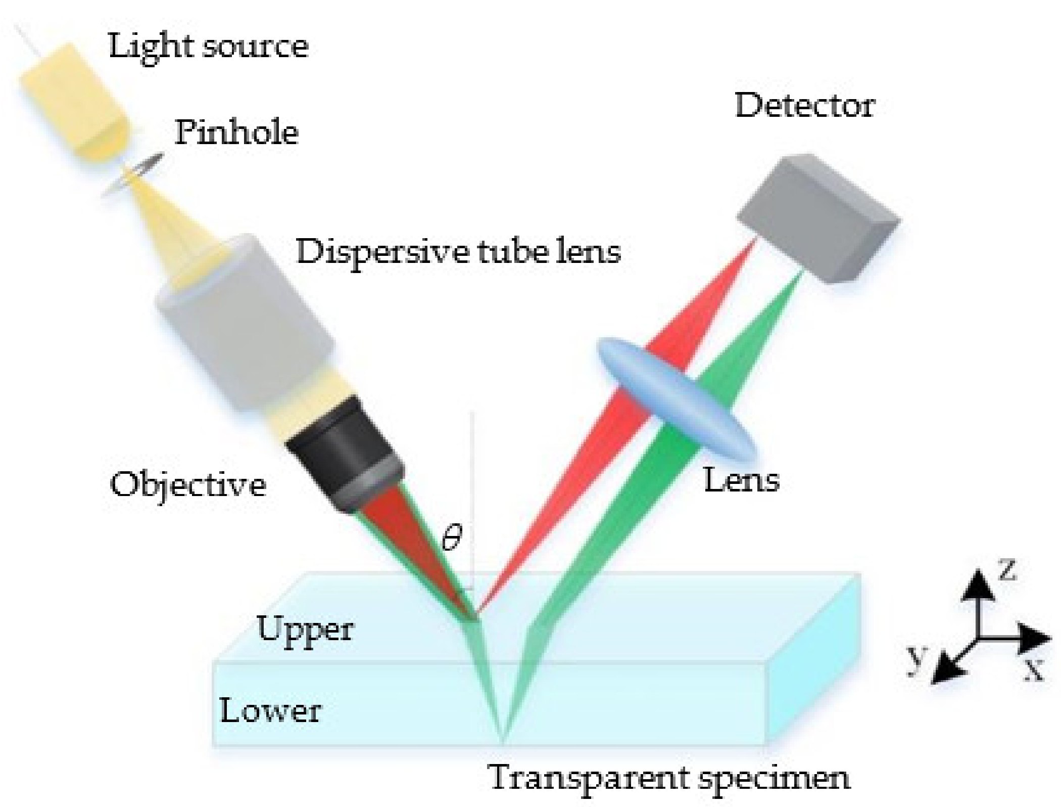
2.1. Principle of Chromatic Confocal Measurement

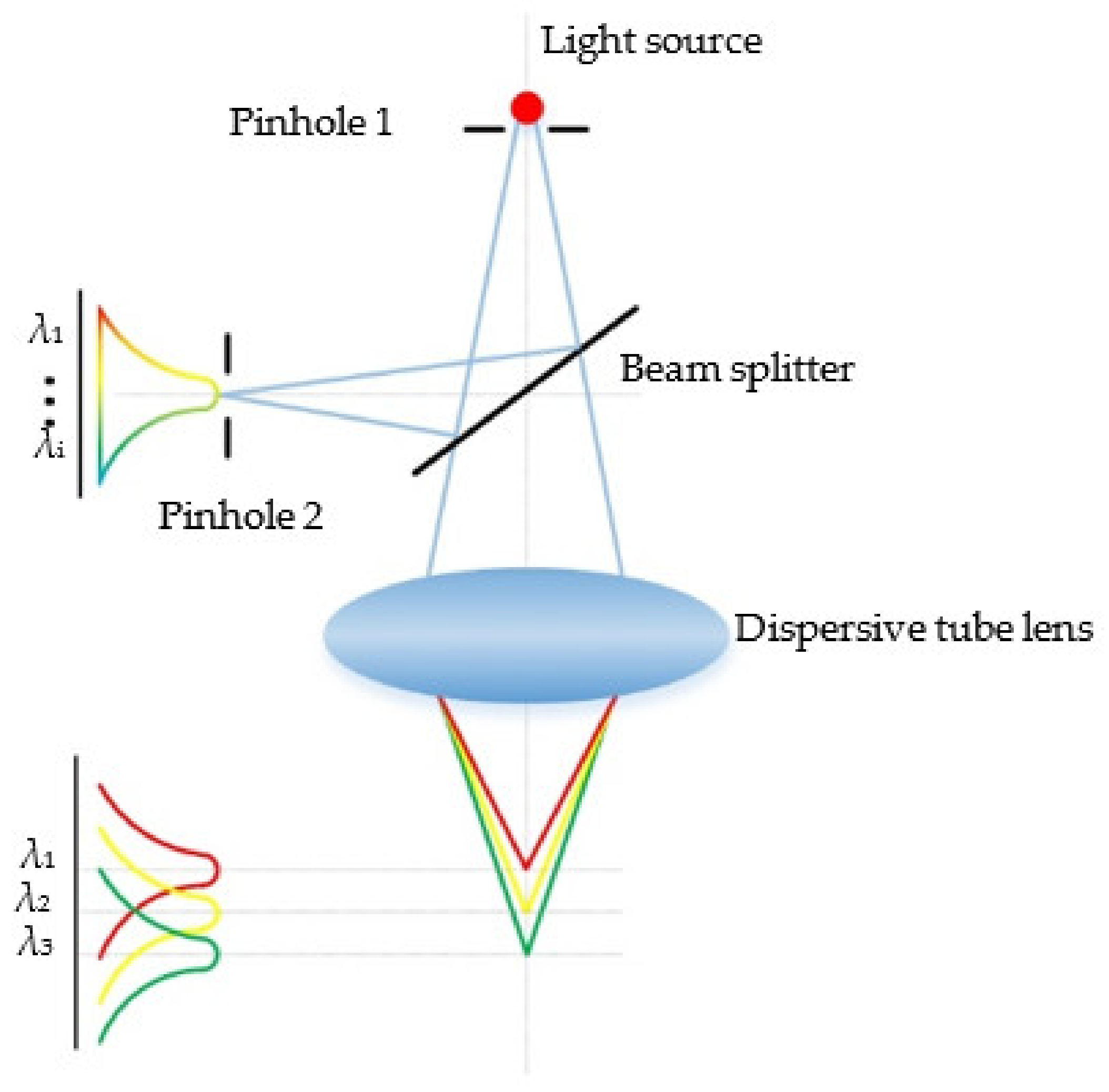
As a non-contact optical measurement method, chromatic confocal technology uses a spectral decoding technology, which is a height/displacement measurement without axial motion, as shown in Figure 1. By establishing the corresponding relation between the axial position of the focal spot and the central wavelength of the focused light, the height/displacement values can be calculated. The schematic diagram of chromatic confocal technology is shown in Figure 2. The polychromatic light source generates multiple wavelength components. The polychromatic light beam passes through a pinhole (pinhole 1 in Figure 2), which modulates the light beam into a point light. Then, the light beam will enter the dispersive tube lens and be distributed along the optical axis according to the different wavelengths. Light beams with different wavelengths will be focused on different positions along the optical axis. Being reflected by the specimen surface, the light beam arrives at the beam splitter and then passes through the detection pinhole (pinhole 2 in Figure 2) which allows only one wavelength to pass through. The height of the specimen surface can be obtained by establishing the correlation between the wavelength of the light that reaches the detector and the axial position of the focal spot.

2.2. Principle of Chromatic Confocal Measurement with Inclined Illumination

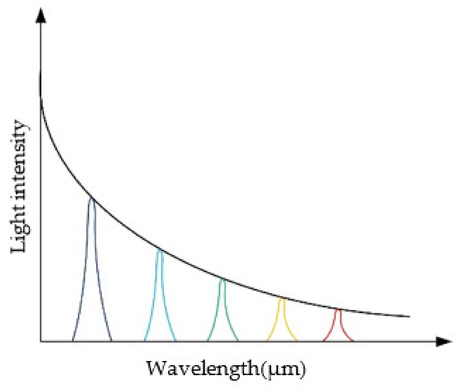
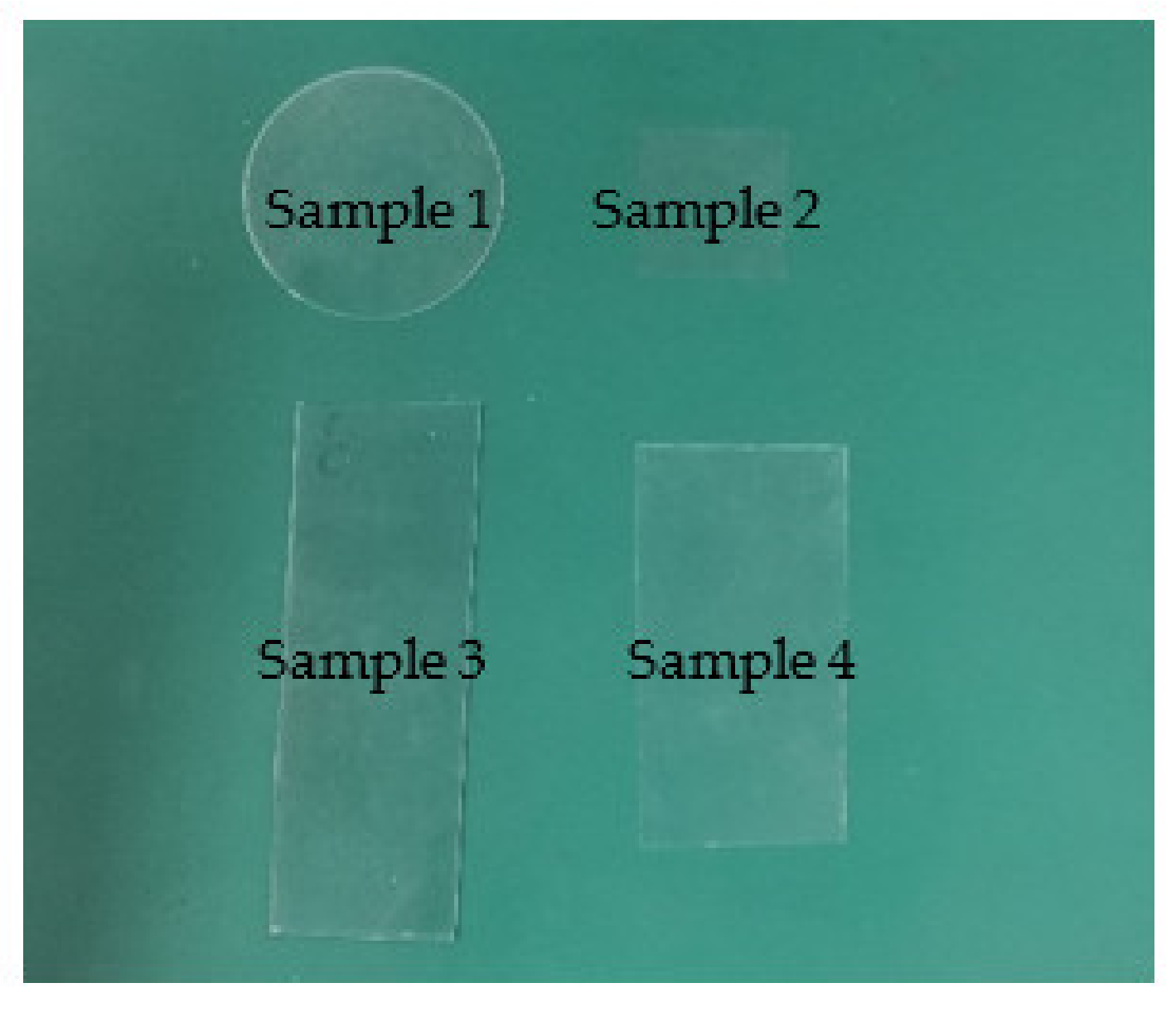
In a conventional chromatic confocal measuring system, the optical axis is set to be perpendicular to the specimen surface. When measuring a transparent specimen surface, it needs to obtain the wavelength values of the light beams which are focused on the upper and lower surfaces, respectively. However, when measuring transparent specimen, the reflecting light intensity will be very weak, as shown in Figure 3. Beam splitters used in such configuration will further lower the effectiveness of energy down to 25%. As a result, the signal-to-noise ratio will be very low.

To solve this problem, an inclined illumination lighting path was developed to the chromatic confocal measurement system, as shown in Figure 4.

The light beams distributed by the dispersive tube lens illuminate the specimen surface with a non-zero incidence angle θ. Compared with the vertical illumination, the extraction of wavelength will be more accurate since the signal-to-noise ratio can be significantly improved.

2.3. Thickness Calculation Model of Glass Slide

In a conventional chromatic confocal measurement system (Figure 5), the normalized light intensity at the focal point can be expressed as follows:

$$I(u)={[\frac{\pi a^2}{\lambda f}\sin c(\frac{u}{4})]}^4$$

(1)

where u is the normalized axial coordinate, λ is the wavelength of the incident light, a is the exit pupil radius of the imaging lens, and f represents the focal length of the lens.

The normalized axial coordinate u can be expressed as follows:

$$u=\frac{2\pi }{\lambda }\Delta z\frac{a^2}{f^2}$$

(2)

In Equation (2), Δz is the defocusing amount, which is determined by the response function of axial light intensity in a chromatic confocal measurement system.

In an ideal chromatic confocal system, the axial position has a linear relationship with the wavelength value of the focused light. For a beam of light with a wavelength λ_i, the defocusing amount is:

$$\Delta h=f\left({\lambda }_i\right)-f\left({\lambda }_0\right)=k\left({\lambda }_{\mathrm{i}}-{\lambda }_0\right)$$

(3)

where f(λ_i) represents the optical axial position, λ_i represents the wavelength of the focused light.

In Figure 4, the incline angle between the optical axis of illumination path and the normal direction of the specimen surface is defined as θ. Thus, the relationship between Δh and Δz(λ_i) can be expressed as follows:

$$\Delta z\left({\lambda }_{\mathrm{i}}\right)=\Delta h·\cos \theta$$

(4)

Substituting Equations (3) and (4) into Equation (1), the light intensity of the detector in Figure 4 can be expressed as follows:

$$I(u)={[\frac{\pi a^2}{{\lambda }_{\mathrm{i}}\left(h_0+k{\lambda }_{\mathrm{i}}\right)}\sin c(\frac{\pi a^{2}k\left({\lambda }_{\mathrm{i}}-{\lambda }_0\right)\cos \theta }{2{\lambda }_{\mathrm{i}}{(h_0+k{\lambda }_{\mathrm{i}})}^2})]}^4$$

(5)

The light intensity distribution of Equation (4) is simulated, which is shown in the black curve in Figure 6. At the same time, the light intensity distribution curves of different wavelengths are simulated, and it can be found that the black curve consists of all peak points of light intensity at every wavelength. As a result, the chromatic confocal system with inclined illumination also has good spectral frequency selection characteristics.

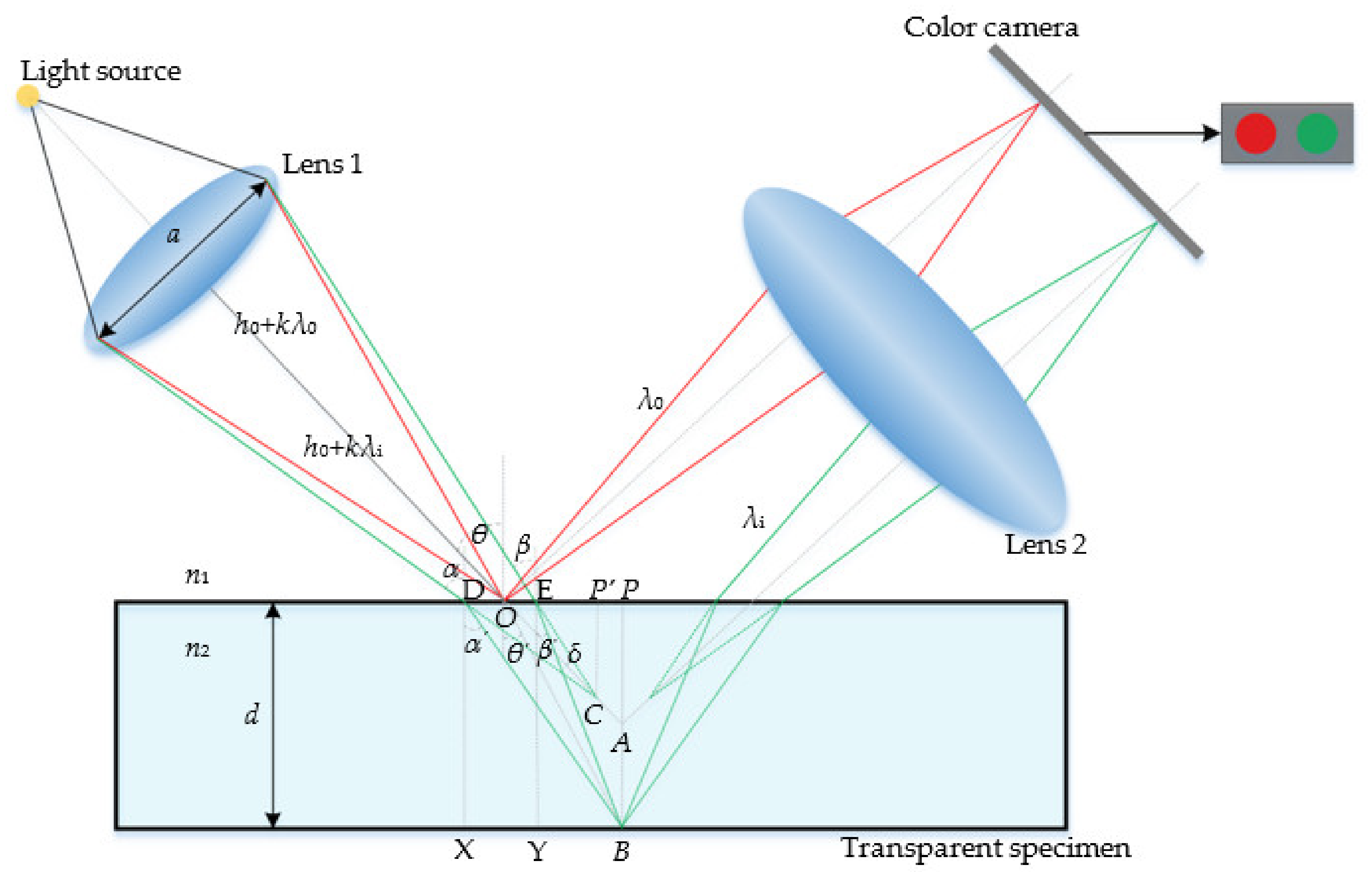
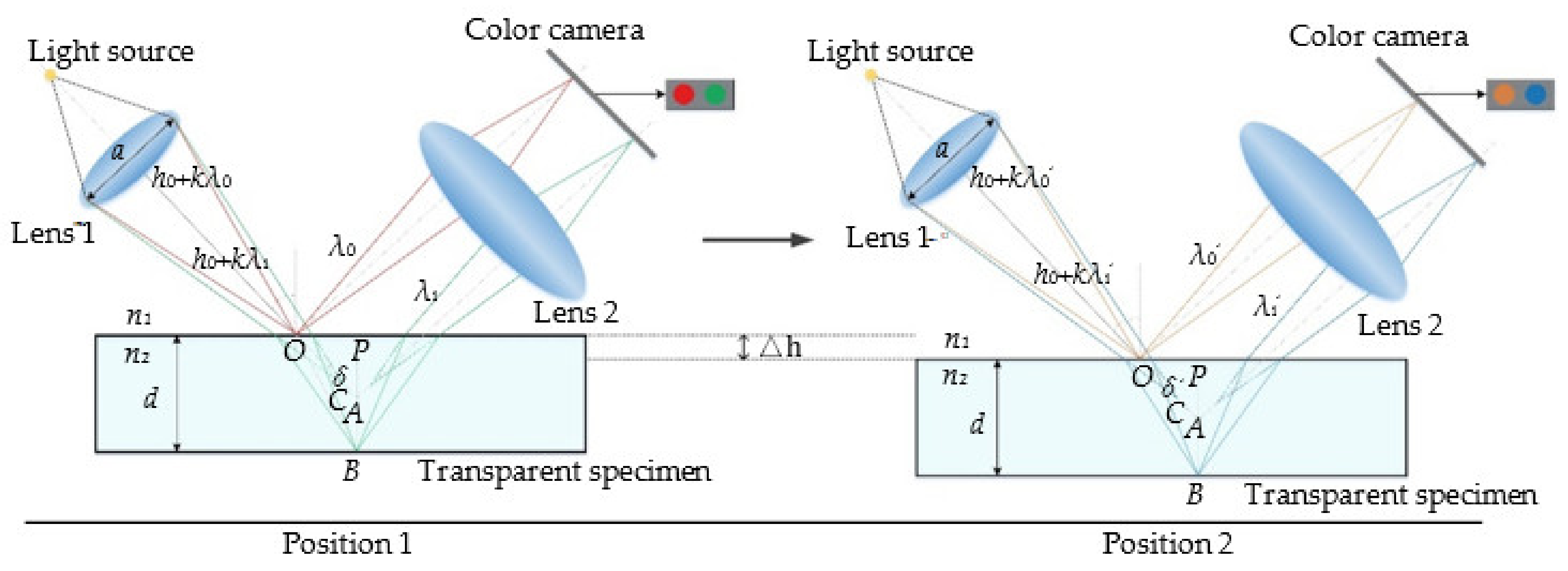
Based on this theoretical analysis, the thickness calculation model of a chromatic confocal system with inclined illumination is provided in the following paragraphs.

As shown in Figure 7, there are two beams of light (wavelength λ₀ and λ_i) focused on the upper and lower surfaces and the focal points are points O and B, respectively. If there was no transparent specimen, the light beam with the wavelength λ_i would be focused on point C. However, it is focused on the lower surfaces due to the existence of transparent specimen.

According to the trigonometric function, the following formula can be obtained:

$$\frac{DE}{d}=\frac{XB-YB}{d}=\tan {\alpha }^{\prime }-\tan {\beta }^{\prime }$$

(6)

$$\frac{DE}{C{P}^{\prime }}=\frac{D{P}^{\prime }-E{P}^{\prime }}{C{P}^{\prime }}=\tan \alpha -\tan \beta$$

(7)

Additionally, the thickness of the transparent specimen d and related parameters can be expressed as:

$$d=C{P}^{\prime }·\frac{\tan \alpha -\tan \beta }{\tan {\alpha }^{\prime }-\tan {\beta }^{\prime }}=OC·\cos \theta ·\frac{\tan \alpha -\tan \beta }{\tan {\alpha }^{\prime }-\tan {\beta }^{\prime }}$$

(8)

Substituting Equation (3) into Equation (8),

$$d=k\left({\lambda }_{\mathrm{i}}-{\lambda }_0\right)·\cos \theta ·\frac{\left(\tan \alpha -\tan \beta \right)}{\left(\tan {\alpha }^{\prime }-\tan {\beta }^{\prime }\right)}$$

(9)

α and β can be calculated by θ and δ:

$$\left\{\begin{array}{c}\alpha =\theta +\delta \\ \beta =\theta -\delta \end{array}\right.$$

(10)

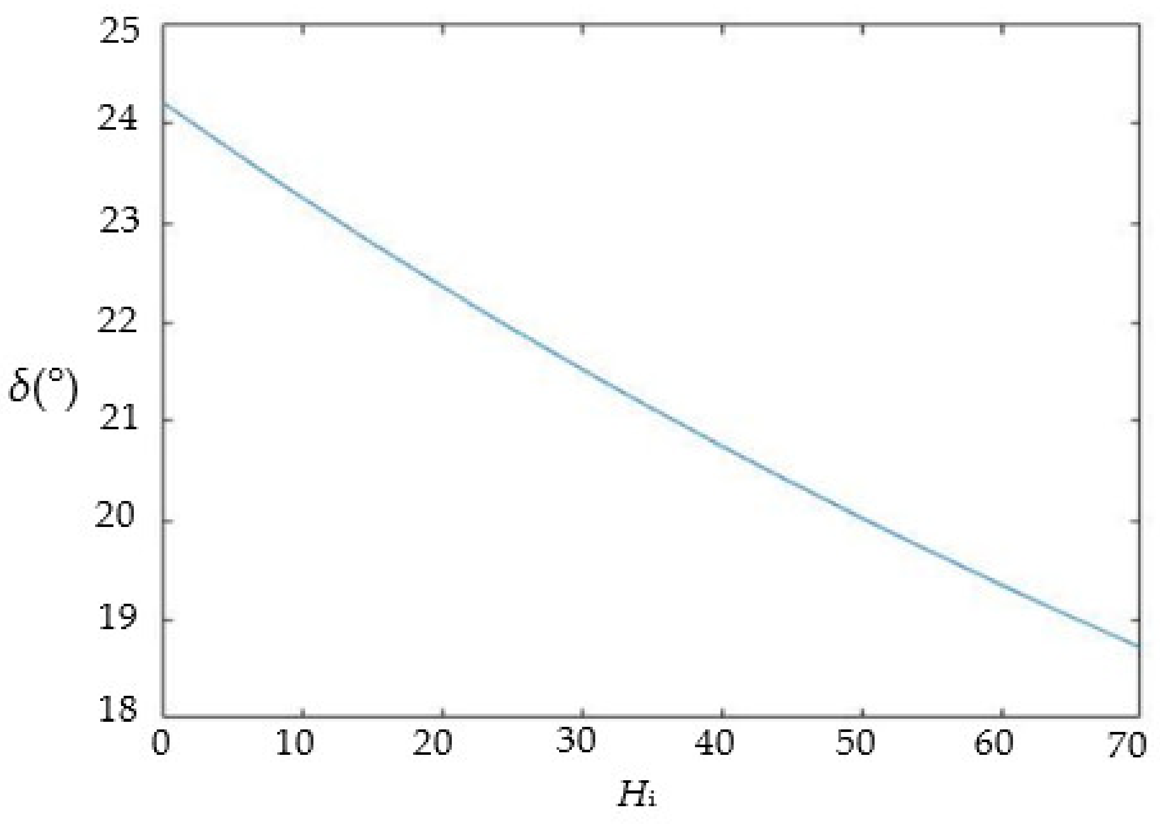
δ is related to the diameter of the dispersion tube lens and the distance from point O to the dispersion tube lens. In this system, a and h₀ can represent the two values. Therefore, δ can be expressed as follows:

$$\delta =\arctan \left[\frac{a}{2(h_0+k{\lambda }_{\mathrm{i}})}\right]$$

(11)

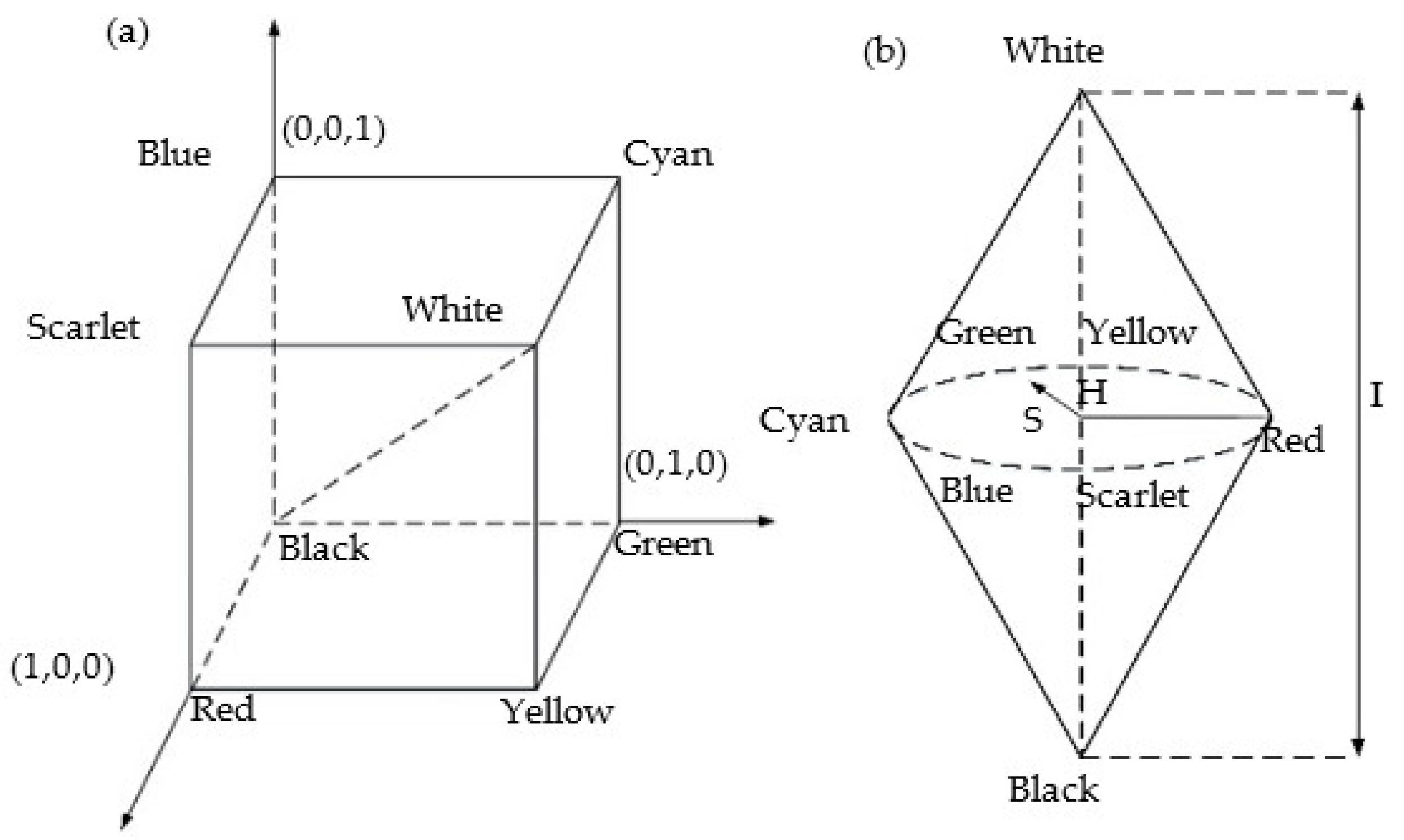
2.4. Color Conversion Algorithm

The image shows different colors because it contains R, G, B values. As discussed in the above sections, the axial displacement of the specimen is related to the wavelength value of the focused light. Therefore, it is necessary to convert color information into wavelength information and a conversion algorithm is proposed to convert RGB space into HSI space, where the H value is correlated with the wavelength. So, H value can be directly used to represent wavelength value. The two color spaces are shown in Figure 8.

In the HSI space, H can be expressed as follows:

$$H=\left\{\begin{array}{cc}\theta ,& G\ge B\\ 2\mathsf{\pi }-\theta ,& G<B\end{array}\right.$$

(12)

where θ is expressed as follows:

$$\theta ={\cos }^{-1}\left(\frac{(R-G)+\left(R-B\right)}{2\sqrt{{\left(R-G\right)}^2+(R-B)(G-B)}}\right)$$

(13)

It has been proved, theoretically and experimentally, that this color conversion algorithm can achieve micron resolution. Additionally, several articles [20,21] have been published using this color conversion algorithm.

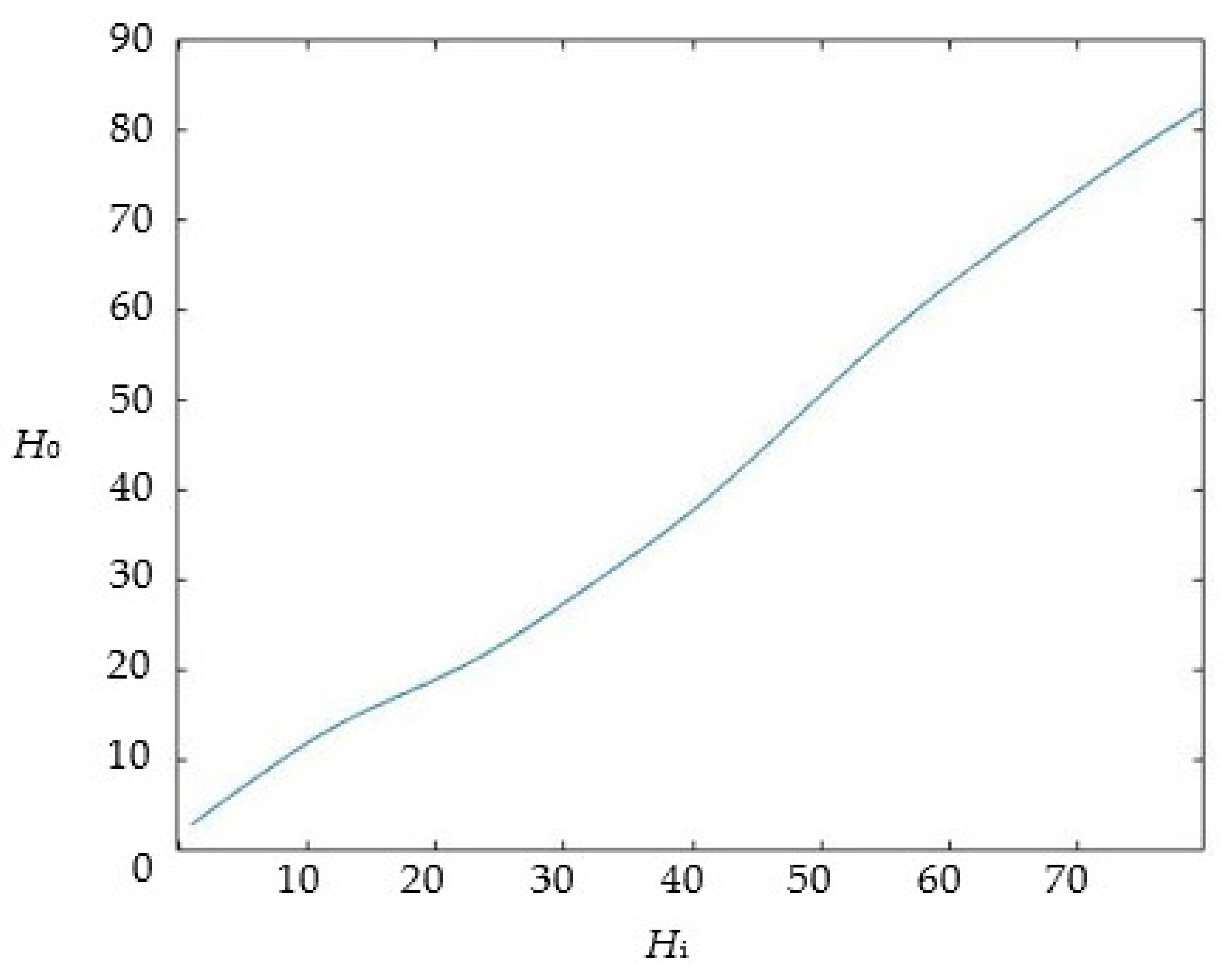
Based on the above, the wavelength can be replaced by H value. Therefore, Equation (3) will become:

$$\Delta h=k_1\left(H_{\mathrm{i}}-H_0\right)$$

(14)

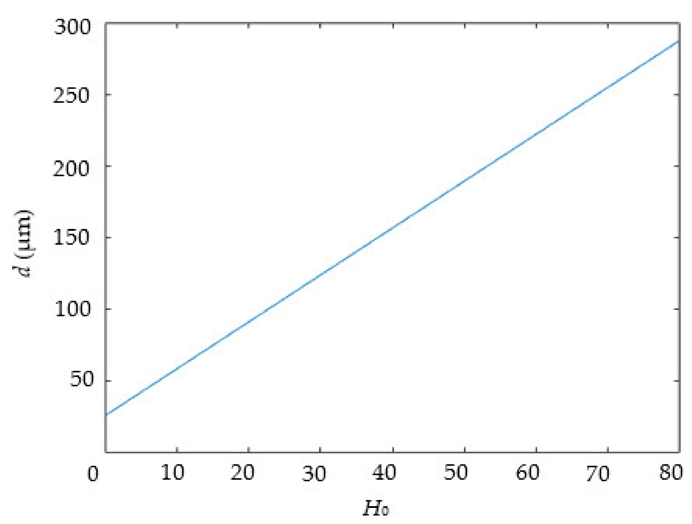
Additionally, the thickness of the transparent specimen d becomes the following:

$$d=k_1(H_{\mathrm{i}}-H_0)\cos \theta \frac{(\tan \alpha -\tan \beta )}{(\tan {\alpha }^{\prime }-\tan {\beta }^{\prime })}$$

(15)

3. Setup and Calibration Experiment of the System

3.1. Setup of the System

Based on the theoretical analysis mentioned above, a chromatic confocal measurement device with inclined illumination was built, as shown in Figure 9. In this device, the polychromatic light beam was distributed by the self-built dispersive tube lens. The angle θ was determined by the angle measuring instrument, which was 43°. The transparent specimen was placed on a two-dimensional motion platform which consists of one-dimensional motion platforms and can move in the directions of arrows shown in Figure 9. The color camera was applied as the receiver to obtain the information of focal spots in the reflected light path. The components used in this device are listed in

Table 1. List of components in the experimental platform.

Components	Manufacturer
Light source	Ocean Optics; HL-2000-FHSA
Dispersive tube lens	Self-built
Objective	Motic;Magnification:10×, NA value:0.25
Two-dimensional motion platform	Daheng Optics; GCM-T25MC
Inductance micrometer	Tesa; TT80
Color camera	Balser; a2A5320-23ucBAS

.

3.2. Calibration Experiment of the System

In order to establish the relationship between the position of the specimen surface and the information of the image color, a calibration experiment was performed in this study.

In this experiment, a transparent specimen was chosen as the test sample. The aberrations [22] have been included in the measurement results. Therefore, we treated the aberrations as a systematic error. The sample was moved 23 steps in the direction of the yellow arrow by a two-dimensional motion platform. At the same time, the camera captured 23 color images at different positions and the inductance micrometer recorded the data of each position. The images were converted to H values by the color conversion algorithm. At last, a relationship between H value and the position was established. The interval of the 23 positions was 100 μm, and the total moving distance was 2200 μm.

Figure 10 shows the color information of the light spots which focused on the upper and lower surfaces. “The upper” in Figure 10 represents the color change reflected from the upper surface of the transparent specimen. “The lower” in Figure 10 represents the color change reflected from the lower surface of the transparent specimen. From position 1 to position 23, the color of the light spot gradually changed from red to green. In the calibration experiment, only the images from the upper surface of the side were recorded and processed.

The H values of 23 focused spots were calculated through color conversion algorithm. Correspond the H value to the data of the positions and note it in

Table 2. Calibration result calculated using the date from the upper surface of the sample.

Axial Displacement (μm)	H Value
0	20.40
100	20.89
200	21.43
300	22.05
400	22.61
500	23.88
600	24.84
700	26.13
800	27.48
900	28.97
1000	30.33
1100	31.93
1200	33.58
1300	35.34
1400	36.57
1500	38.60
1600	40.90
1700	43.50
1800	46.73
1900	50.65
2000	55.12
2100	60.77
2200	65.57

. The calibration curve before fitting is shown in Figure 11a. Within 700–1500 μm, 9 points were selected for linear fitting, as shown in Figure 11b.

In the linear fitting, the standard square value of the fitting curve was 0.99, and the relationship between the axial displacement of the sample f(H) and the H value is as below:

$$f\left(H\right)=64.30H-964.09$$

(16)

4. Error Theory Analysis and Correction

4.1. Error Theory Analysis

In Section 2.3, the thickness calculation model of the transparent specimen is derived. The thickness of the transparent specimen depends on multiple parameters, such as the wavelength value of the light beams focused on the upper and the lower surfaces, the incidence angle θ and the conic focusing angle δ. The angle incidence θ is a constant in this system. However, as the sample moves within the measurement range, the wavelength value of the light beams focused on the upper and lower surfaces and the angle δ change gradually.

Figure 12 shows the scenario that the sample is measured in different positions. When the sample is at position 1, the wavelength value of the light beams focused on the upper and lower surfaces are λ₀ and λ_i. When the sample moves to position 2, the wavelength value of the focused light becomes λ₀′ and λ_i′. The conic focusing angle δ becomes to a smaller angle δ′. According to Equation (15), the thickness d will change as the wavelength value and the focusing angle δ have changed.

In order to further study the correctness and feasibility of the error theory as mentioned above, it is needed further validation by simulated analysis. During the simulation, the thickness d is set as 175.00 μm. The settings of other parameters are shown in

Table 3. The setting of parameters.

Parameter	Value
a (μm)	9000.00
h0 (μm)	10,000.00
δ (°)	20.00
θ (°)	43.00
k	64.30
n1	1.00
n2	1.50

.

Equation (17), derived from Equation (15), can be seen as the functional relation between H₀ and H_i:

$$H_{\mathrm{i}}=H_0+\frac{d(\tan {\alpha }^{\prime }-\tan {\beta }^{\prime })}{k\cos \theta (\tan \alpha -\tan \beta )}$$

(17)

Equation (17) shows that H₀ and H_i are approximately linear.

Since the angle δ is a variable value, the constant terms in Equation (17) do not remain constant. Using the data in Table 3 to simulate Equation (17), the result is shown in Figure 13.

The following formula can be obtained by linear fitting the data in Figure 13:

$$H_0=1.05H_{\mathrm{i}}-4.18$$

(18)

This shows that the H values of the light beams focused on the upper and lower surfaces have a good linearity when the sample is at different positions.

In order to verify the difference of measurement results in different positions, the thickness d in Equation (15) is simulated, as shown in Figure 14. To indicate that the sample is in different positions, the value of H₀ is set from 0 to 80. The value of H_i can be calculated by Equation (18) and other parameters in Table 3.

The simulation result in Figure 14 shows that the thickness d gradually decreases as H₀ increases; in other words, as the sample moves away from the incident light. This simulation result shows there is certain measurement error in different positions. The thickness d is also related to the angle δ. Then, Equation (10) is simulated as parameters set according to Table 3.

It can be seen from Figure 15 that the angle δ gradually decreases when the sample moves away from the incident light, which is consistent with the geometric analysis result in Figure 12.

4.2. Error Correction

According to the error theoretical analysis in Section 4.1, the measurement error of the thickness d comes from the change of the angle δ in different positions. Therefore, accurately determining the value of the angle δ in different positions is the key to improving the precision of the system, reducing the error and achieving measurement in different positions.

In Section 2.3, the axial position has a linear relationship with the wavelength value of the focused light and the wavelength value can be converted to H value. Then, Equation (10) can be expressed as:

$$\delta =\arctan \left[\frac{a}{2(h_0+k_1{H}_{\mathrm{i}})}\right]$$

(19)

The angle δ is related to the h₀ and H_i, and the values of the angle δ and the H_i will change as the sample moving. Therefore, it is necessary to determine the accurate value of h₀ and the value of the angle δ in different positions.

The specific steps of the error correction method are as follows:

• After the calibration experiment, the measurement range of the system can be represented by a range of H values. A transparent specimen with known thickness was placed in the system. The upper surface was placed accurately at the starting position of the measurement range and the lower surface must also be within the measurement range. Height values of the light beams focused on the upper and lower surfaces were recorded as H₀ and H_i.
• The values of d, H₀ and H_i were taken into Equations (10) and (15) to calculate the angle δ in this position.
• The angle δ calculated in step 2 was taken into Equation (19) to find h₀ which was set as the original parameters of the system.
• When measuring in different positions, the H_i value of the light beams focused on the lower surface in the current position was recorded. The angle δ of the current position then was calculated using Equation (19).
• The thickness in each position was calculated by using the data of the H₀, H_i and δ in the current position.

5. Thickness Measurement Experiments of the Transparent Specimens

In Section 2.2, the calculation formula for the thickness of the transparent specimen has been proposed. This section will provide the experimental details in this study. Using the experimental platform shown in Figure 9, the calibration work was performed. Then, three kinds of transparent specimens with different thicknesses and refractive indexes were measured. The physical images of Sample 1, Sample 2, Sample 3 and Sample 4 are shown in Figure 16. Sample 1 was used to calculate the initial parameters and angles of the system, and Sample 2, 3 and 4 were used as experimental samples to measure the thickness with the error correction model. Sample 2 is made of glass, Sample 3 is made of PVC and Sample 4 is made of PET. Additionally, the true thickness values of Samples 2, 3 and 4 are 172.54 μm, 679.72 μm and 245.00 μm, respectively, which are measured by a universal length measuring machine and its product model is TRIMOS LABC500. The universal length measuring machine is shown in Figure 17.

Firstly, according to the error theoretical mentioned in Section 4.2, Sample 1 was selected to determine the initial parameter h₀ of the system. Sample 1 was placed in the starting position within the linear range of the system. The parameters of the system are listed in

Table 4. Fixed parameters in the system.

Parameter	Value
θ (°)	43.00
δ0 (°)	30.89
h0 (μm)	5695.53

.

Then, the thicknesses of Samples 2, 3 and 4 were measured, respectively, and the experiment of each sample was repeated 15 times in different positions within the measurement range. The measurement data of Samples 2, 3 and 4 were listed in the following tables. In each table, the measurement data with and without correction were provided (The thicknesses without correction were calculated through the angle δ₀ in Table 4).

5.1. Glass Specimen

When using glass such as Samples 2 as the specimen, the value of refractive index n₂ is 1.50.

Figure 18 shows one of the 15 captured pictured in the measurement of Sample 2. Using the color conversion algorithm, the R, G, and B information of these 15 pieces of pictures were converted to H values. According to the correction method in Section 4.2, the angle δ was calculated and thickness d was calculated according to Equations (8) and (13), as listed in

Table 5. Experimental data of the thickness of Sample 2.

Position Number	H Value of Upper Surface	H Value of Lower Surface	Value of Difference	Angle δ (°)	Thickness without Correction d’ (μm)	Thickness with Correction d (μm)
1	27.64	28.43	0.79	30.88	174.99	174.93
2	28.21	29.00	0.79	30.76	174.51	173.43
3	28.46	29.27	0.81	30.70	178.48	176.90
4	29.32	30.13	0.81	30.52	177.91	174.82
5	29.56	30.38	0.82	30.47	180.65	177.07
6	29.95	30.76	0.81	30.39	178.01	173.84
7	30.33	31.16	0.83	30.30	181.19	176.27
8	30.68	31.50	0.82	30.23	180.52	175.05
9	31.53	32.36	0.83	30.06	182.88	175.92
10	31.95	32.80	0.85	29.97	186.11	178.30
11	32.60	33.43	0.83	29.84	184.25	175.51
12	33.79	34.64	0.85	29.60	187.55	176.76
13	34.56	35.42	0.86	29.44	190.69	178.52
14	35.64	36.51	0.87	29.23	192.90	178.95
15	36.83	37.70	0.87	28.99	192.40	176.77
The average value of the thickness with correction (μm)		176.20		Standard deviation σ of d’ (μm)		5.97
				Standard deviation σ of d (μm)		1.64

.

The thickness measurement data of Sample 2 was shown in Table 5.

The calculation formula of the standard deviation σ is:

$$\sigma =\sqrt{\frac{{\displaystyle \sum {\left(x_i-\overline{x}\right)}^2}}{n-1}}$$

(20)

Figure 19 showed the measurement results of Samples 2. It was obviously that the measurement results with correction had a smaller error than those without correction.

With correction, the thickness of Sample 2 was 176.26 μm and the repeatability decreased from 11.94 μm to 3.28 μm. The measurement error was 2.12%.

5.2. PVC Specimen

When using PVC such as Sample 3 as the specimen, the value of refractive index n₂ is 1.55. Additionally, the thickness measurement data and result of Sample 3 are shown in

Table 6. Experimental data of the thickness of Sample 3.

Position Number	H Value of Upper Surface	H Value of Lower Surface	Value of Difference	Angle δ (°)	Thickness without Correction d’ (μm)	Thickness with Correction d (μm)
1	27.80	30.83	3.03	30.37	713.92	691.77
2	28.16	31.19	3.04	30.30	715.81	691.18
3	29.23	32.33	3.10	30.06	729.44	696.87
4	30.13	33.22	3.09	29.88	726.65	688.55
5	30.26	33.38	3.12	29.85	735.97	696.35
6	30.62	33.71	3.09	29.78	726.60	685.50
7	31.07	34.17	3.10	29.69	730.59	686.43
8	31.51	34.65	3.14	29.59	740.35	692.71
9	32.11	35.25	3.14	29.47	739.57	688.46
10	32.51	35.63	3.12	29.40	734.63	681.64
11	33.46	36.60	3.14	29.21	739.28	680.39
12	34.01	37.18	3.17	29.09	745.83	683.23
13	35.41	38.64	3.23	28.82	760.31	688.49
14	35.71	38.97	3.26	28.75	768.28	693.92
15	38.06	41.32	3.26	28.31	768.72	682.25
The average value of the thickness with correction (μm)			688.52		Standard deviation σ of d’ (μm)	16.69
					Standard deviation σ of d (μm)	5.27

and Figure 20, respectively.

With correction, the thickness of Sample 3 was 688.52 μm and the repeatability decreased from 33.38 μm to 10.54 μm. The measurement error was 1.29%.

5.3. PET Specimen

When using PET such as Sample 4 as the specimen, the value of refractive index n₂ is 1.65. The thickness measurement data and result of Sample 4 are shown in

Table 7. Experimental data of the thickness of Sample 4.

Position Number	H Value of Upper Surface	H Value of Lower Surface	Thickness without Correction d’ (μm)	Thickness with Correction d (μm)
1	28.54	29.50	247.99	248.02
2	28.60	29.56	246.65	246.54
3	29.25	30.22	250.71	248.72
4	29.30	30.26	249.25	247.16
5	29.49	30.45	248.57	245.97
6	29.83	30.79	249.11	245.57
7	30.68	31.66	251.65	245.77
8	30.70	31.69	257.14	251.05
9	31.08	32.09	260.23	252.99
10	31.80	32.82	263.08	253.83
11	33.26	34.28	262.29	249.37
12	34.46	35.48	262.96	247.11
13	35.86	36.89	268.95	249.39
14	36.51	37.56	271.52	250.26
15	37.28	38.34	271.46	248.48
The average value of the thickness with correction (μm)		248.68	Standard deviation σ of d’ (μm)	8.95
			Standard deviation σ of d (μm)	2.53

and Figure 21, respectively.

With correction, the thickness of Sample 4 was 248.68 μm and the repeatability decreased from 17.90 μm to 5.06 μm. The measurement error was 1.50%.

As shown in Figure 19, Figure 20 and Figure 21, when the Samples were placed at different positions, the measurements without correction showed increasing measurement errors, leading to a significant measurement uncertainty (represented by standard deviation). In contrast, when the proposed correction method was applied, the measurement results showed significantly improved position independence. At the same time, the correction method has good correction effect on the samples with different refractive indexes.

6. Discussion

• Experimental results showed that axial measurement accuracy of the system could reach the micron level and the measurement errors were significantly reduced, as compared to the uncorrected system.
• The relationship between the thickness d and the angle δ was discussed and derived in this paper. We calculated the value of h₀ of the system, which was 5695.53 μm.
• It was found that the parameters of the system were inconsistent when the transparent specimen at different positions. Additionally, an error correction model was proposed by calculating the parameter values.
• The transparent specimens used in this experiment were made of different materials such as glass, PVC and PET. Additionally, a series of experiments were conducted using the error correction model.

7. Conclusions

In the fields of thickness measurement of transparent specimen, the chromatic confocal system with inclined illumination is able to achieve better signal-to-noise ratio. However, the measurement results at different axial positions vary significantly.

In this paper, position-induced error was analyzed. It was found that the parameters of the confocal model are inconsistent when the sample is axially moving. Based on this finding, an error correction model was proposed by calculating the parameter values at different positions. Using this error correction, a series of experiments were conducted with transparent specimens made of different materials such as glass, PVC, and PET. The experimental results showed that the correction could effectively correct the measurement error induced by the position change. Therefore, the measurement accuracy can be effectively improved.