Quantum Speed Limit for a Moving Qubit inside a Leaky Cavity

Abstract

The quantum speed limit (QSL) is a theoretical lower bound of the time required for a quantum system to evolve from an arbitrary initial state to its orthogonal counterpart. This figure can be used to characterize the dynamics of open quantum systems, including non-Markovian maps. In this paper, we investigate the QSL time for a model that consists of a single qubit moving inside a leaky cavity. Notably, we show that for both weak and strong coupling regimes, the QSL time increases while we boost the velocity of the qubit inside the leaky cavity. Moreover, it is observed that by increasing the qubit velocity, the speed of the evolution tends to a constant value, and the system becomes more stable. The results provide a better understanding of the dynamics of atom-photon couplings and can be used to enhance the controllability of quantum systems.

1. Introduction

Quantum mechanics, as a fundamental law in nature, sets a bound on the speed of evolution of a quantum system. This bound is utilized in various topics of quantum theory, including quantum communication [1], the investigation of accurate bounds in quantum metrology [2], computational bounds of physical systems [3] and optimal quantum control algorithms [4]. The shortest time a system needs to change from an initial state to its orthogonal state is called the quantum speed limit (QSL) time. This time has been studied for both closed and open quantum systems. For closed systems, geometric criteria such as the Bures angle and relative purity are used to define the bound of QSL time [5,6,7,8,9,10,11,12]. The first bound of QSL time for closed quantum systems was introduced by Mandelstam and Tamm as [11]

$${\tau }_{QSL}^{\mathrm{MT}}=\frac{\pi ħ}{2\mathrm{\Delta }E},$$

(1)

where $\mathrm{\Delta }E=\sqrt{\langle {\widehat{H}}^2\rangle -{\langle \widehat{H}\rangle }^2}$ is the variance of energy of the initial state and $\widehat{H}$ shows the time-independent Hamiltonian. The bound in Equation (1) is known as the MT bound. Another bound of QSL time for closed quantum systems was introduced by Margolus and Levitin as [12]

$${\tau }_{QSL}^{\mathrm{ML}}=\frac{\pi ħ}{2E},$$

(2)

where $E=\langle \widehat{H}\rangle$. The bound in Equation (2) is known as the ML bound. In Ref. [7], Giovannetti et al. combine the MT and ML bounds for closed quantum systems and introduce a unified bound for the QSL time as [13]

$${\tau }_{QSL}=max\left\{\frac{\pi ħ}{2\mathrm{\Delta }E},\frac{\pi ħ}{2E}\right\}.$$

(3)

In the real world of quantum mechanics, we are dealing with open systems. Hence, the investigation of these systems is of particular importance [14,15,16]. Thus far, a lot of works have been done on QSL time for open quantum systems [17,18,19,20,21,22,23,24,25,26,27,28,29,30,31,32,33,34,35,36,37,38,39,40,41,42,43,44,45,46,47,48]. For instance, Fogarty et al. [17] have shown that the dynamics of orthogonality catastrophe can be characterized by the QSL. In Ref. [18], the authors have demonstrated that the QSL for counterdiabatically driven systems experiencing quantum phase transitions completely encodes the Kibble–Zurek mechanism by precisely predicting the transition from adiabatic to impulse regimes. More recently, Campaioli et al. [41] have constructed bounds on the minimum time required for a provided resource to alter through a fixed increment by utilizing the toolkit of QSLs.

It has been shown that the bound of QSL time for open quantum systems can be defined by extending the MT and ML bounds for these systems [7,8]. In Ref. [28], Zhang et al. have introduced the bound for open quantum systems based on the relative purity for an arbitrary initial state. They have shown that QSL time is dependent on quantum coherence. In this work, we use the Zhang et al. bound, which is presented in Section 3. The motivation for using this bound here is that it can be used for any desired initial state.

The scheme of recent experiments in quantum information theory is based on the control of a qubit within a cavity. In practice, it is difficult to achieve the static state of a qubit in a cavity. Many studies have been done about the moving qubits in Markovian and non-Markovian environments [49,50,51,52,53,54]. Markovian evolution is a memory-less evolution in which information is monotonically leaked from the system to the environment, and there is no backflow of information from the system to the environment. On the other hand, in the non-Markovian regime, the information flows back from the environment to the system. The protection of initial entanglement by moving two qubits in a non-Markovian environment has been studied in Ref. [50]. In Ref. [49], the effects of qubit velocity within the leaky cavity on quantum coherence protection have been studied. The dependence of QSL time on quantum coherence motivates us to study the effect of qubit velocity in a leaky cavity on QSL time. The motivation for choosing this model is that in recent works, it has been shown that by increasing the qubit velocity inside the leaky cavity, the coherence of the qubit state is further protected. Therefore, we expect that as the qubit velocity increases within the leaky cavity, the QSL time will increase, and evolution will be slower.

The work is organized as follows. In Section 2, the model is introduced. In Section 3, the QSL time for a moving qubit is investigated. We disclose the significance and prospects of the current study in Section 4. Finally, we provide conclusions in Section 5.

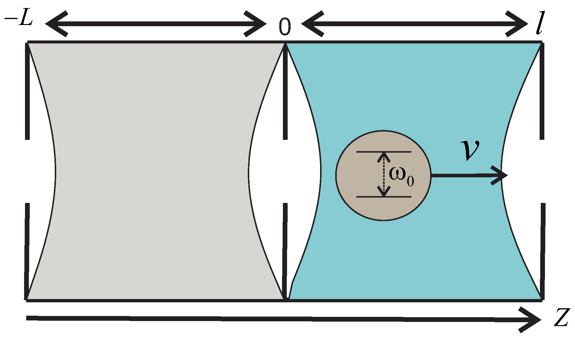
2. Moving Qubit inside a Leaky Cavity

Here, let us consider a model that includes a single-qubit system and a structured environment. The structure of the environment consists of two mirrors, one at $z=-L$ and the other at $z=l$. There is also a mirror with partial reflection at $z=0$. It can be said that the environment consists of two consecutive cavities in intervals $(-L,0)$ and $(0,l)$. The structure of the model is shown in Figure 1. The qubit moves in both cavities; however, the qubit is taken to interact only with the second cavity $(0,l)$ and moves along the z-axis with constant velocity. Any classical electromagnetic field, namely $E(z,t)$ in $(-L,l)$, can be expanded as [49,50]

$$E(z,t)=\sum _k{E}_k\left(t\right)U_k\left(z\right)+E_k^{*}\left(t\right)U_k^{*}\left(z\right),$$

(4)

where $U_k\left(z\right)$ is the accurate monochromatic mode at frequency ${\omega }_k$ and $E_k\left(t\right)$ denotes the amplitude in the k-th mode. Herein, it is assumed that the electromagnetic field is polarized along the x-axis. To meet the boundary conditions in mirrors, the mode functions should be

$$U_k\left(z\right)=\left\{\begin{array}{cc}{\epsilon }_{k}sink(z+L)\hfill & z<0\hfill \\ J_{k}sink(z-l)\hfill & z>0\hfill \end{array}\right.$$

(5)

where ${\epsilon }_k$ takes the value $\pm 1$ going from each mode to the subsequent one, and for a good cavity, we have

$$J_k=\frac{\sqrt{c{\lambda }^2/l}}{\sqrt{{\left({\omega }_k-{\omega }_n\right)}^2+{\lambda }^2}},$$

(6)

where ${\omega }_n=n\pi c/l$ is the frequency of the n-th quasi mode and $\lambda$ represents the damping of the cavity in $(0,l)$. $\lambda$ determines the photon leakage through the cavity mirrors and also determines the spectral width of the spectral density. Here, we assume that the qubit interacts with the second cavity located in the range $(0,l)$. The qubit also moves along the z-axis at a constant speed v. The qubit interacts with the cavity modes as it moves inside the cavity. Considering the dipole and rotating-wave approximation, the Hamiltonian of the system is defined as follows:

$$\begin{array}{cc}\hfill \widehat{H}& ={\omega }_0{|0\rangle }_s\langle 0|+\sum _k{\omega }_k{a}_k^{†}{a}_k+\sum _k{f}_k\left(z\right)\left(g_k{|1\rangle }_s{〈0\left|a_k+g_k^{*}\right|0〉}_s\langle 1|a_k^{†}\right),\hfill \end{array}$$

(7)

where ${|0\rangle }_s$ (${|1\rangle }_s$) is the excited (ground) state of the qubit system, ${\omega }_0$ denotes the transition frequency of the qubit, $a_k^{†}$ ($a_k$) is the creation (annihilation) operator for the k-th cavity mode with the frequency ${\omega }_k$, and $g_k$ specifies the coupling between qubit and cavity. The shape function describing the motion of the qubit along the z-axis is given by [55,56,57]

$$f_k\left(z\right)=f_k\left(vt\right)=sin\left[k(z-l)\right]=sin\left[{\omega }_k(\beta t-\mathcal{T})\right],$$

(8)

where $\beta =v/c$ and $\mathcal{T}=l/c$. It has been shown that the parameter $\beta$ can be expressed as $\beta =v/c=\left(x\right)\times {10}^{-9}$ [49]. It is equivalent to $v=0.3\left(x\right)$ for a ${}^{85}Rb$ Rydberg microwave qubit. Let us assume that the general initial state of the total system is given by

$$|\psi \left(0\right)\rangle =\left(c_1{|0\rangle }_s+c_2{|1\rangle }_s\right)\otimes {|0\rangle }_c,$$

(9)

where we have $|c_1{|}^2+{\left|c_2\right|}^2=1$. The initial state of the cavity is in a vacuum state ${|0\rangle }_c$. After a while, the system state changes to the following form at time t

$$|\psi \left(t\right)\rangle =c_1{A\left(t\right)|0\rangle }_s{|0\rangle }_c+c_2{|1\rangle |0\rangle }_c+\sum _k{B}_k\left(t\right){|1\rangle }_s{\left|1_k\right.〉}_c,$$

(10)

in which ${\left|1_k\right.〉}_c$ is the cavity state that includes one photon in the k-th mode. Using the Schrödinger equation, differential equations for the probability amplitudes $A\left(t\right)$ and $B_k\left(t\right)$ can be obtained as follows:

$$i\dot{A}\left(t\right)={\omega }_{0}A\left(t\right)+\sum _k{g}_k{J}_k{f}_k\left(vt\right)B_k\left(t\right),$$

(11)

$$i{\dot{B}}_k\left(t\right)={\omega }_k{B}_k\left(t\right)+g_k^{*}{J}_k{f}_k\left(vt\right)A\left(t\right).$$

(12)

By solving Equation (12) and putting its results in Equation (11), we will have

$$\dot{A}\left(t\right)+i{\omega }_{0}A\left(t\right)=-{\int }_0^{t}d{t}^{\prime }A\left(t^{\prime }\right)\sum _k{\left|g_k\right|}^2{J}_k^2{f}_k\left(vt\right)f_k\left(v{t}^{\prime }\right)e^{-i{\omega }_k\left(t-t^{\prime }\right)}.$$

(13)

By defining the probability amplitude as $A\left(t^{\prime }\right)=\tilde{A}\left(t^{\prime }\right)e^{i{\omega }_0{t}^{\prime }}$ and putting it into Equation (13), we have

$$\dot{\tilde{A}}+{\int }_0^{t}d{t}^{\prime }F(t,t^{\prime })\tilde{A}\left(t^{\prime }\right)=0,$$

(14)

where the memory kernel $F(t,t^{\prime })$ is defined as follows

$$F(t,t^{\prime })=\sum _k{\left|g_k\right|}^2{J}_k^2{f}_k\left(vt\right)f_k\left(v{t}^{\prime }\right)e^{-i({\omega }_k-{\omega }_0)(t-t^{\prime })}.$$

(15)

This memory kernel in the continuum limit has the following form

$$F(t,t^{\prime })={\int }_0^{\infty }J\left({\omega }_k\right)f_k(t,t^{\prime })e^{-i({\omega }_k-{\omega }_0)(t-t^{\prime })}d{\omega }_k,$$

(16)

where $f_k(t,t^{\prime })=sin\left[{\omega }_k(\beta t-\mathcal{T})\right]sin\left[{\omega }_k(\beta t^{\prime }-\mathcal{T})\right]$ and $J\left({\omega }_k\right)$ represents the spectral density of an electromagnetic field inside the cavity. Let us assume that the spectral density of the electromagnetic field inside a cavity has the Lorentzian form

$$J\left({\omega }_k\right)=\frac{1}{2\pi }\frac{\gamma {\lambda }^2}{{({\omega }_n-{\omega }_k)}^2+{\lambda }^2},$$

(17)

where ${\omega }_k$ shows the frequency of the k-th cavity mode and ${\omega }_n$ is the center frequency of the cavity modes. $\lambda$ is the spectral width of the spectral density, which is related to the cavity correlation time ${\tau }_c$ through ${\tau }_c=1/\lambda$. The parameter $\gamma$ (coupling strength) is related to the scale time ${\tau }_s$, during which the system changes, through ${\tau }_s=1/\gamma$. Strong and weak coupling regimes can be distinguished by comparing both the ${\tau }_c$ and ${\tau }_s$ time scales. When ${\tau }_s>2{\tau }_c$ ($\gamma <\lambda /2$), we have the weak coupling regime, and the dynamics are Markovian [58,59]. The strong coupling regime corresponds to the case in which ${\tau }_s<2{\tau }_c$ ($\gamma >\lambda /2$), where the dynamics iare non-Markovian. In the continuous limit ($\mathcal{T}⟶\infty$), when $t>t^{\prime }$, the memory kernel can be written as

$$F(t,t^{\prime })=\frac{\gamma \lambda }{4}cosh\left[\theta (t-t^{\prime })\right]e^{\overline{\lambda }(t-t^{\prime })},$$

(18)

where $\overline{\lambda }=\lambda -i\mathrm{\Delta }$ and $\theta =\beta (\overline{\lambda }+i{\omega }_0)$. By putting Equation (18) to Equation (14) and using the Bromwich integral formula, the probability amplitudes $\tilde{A}\left(t\right)$ can be obtained as follows:

$$\tilde{A}\left(t\right)=\frac{(q_1+u_{+})(q_1+u_{-})}{(q_1-q_2)(q_1-q_3)}{e}^{q_1\gamma t}-\frac{(q_2+u_{+})(q_2+u_{-})}{(q_1-q_2)(q_2-q_3)}{e}^{q_2\gamma t}+\frac{(q_3+u_{+})(q_3+u_{-})}{(q_1-q_3)(q_2-q_3)}{e}^{q_3\gamma t},$$

(19)

where $q_i$’s ($i=1,2,3$) satisfy the following cubic equation as

$$q^3+2(y_1-i{y}_3)q^2+(u_{+}{u}_{-}+\frac{y_1}{4})q+\frac{y_1(y_1-i{y}_3)}{4}=0,$$

(20)

where $y_1=\lambda /\gamma$, $y_2={\omega }_0/\gamma$, $y_3=({\omega }_0-{\omega }_n)/\gamma$, and $u_{\pm }=(1\pm \beta )\pm i\beta y_2-i(1\pm \beta )y_3$. Using Equation (19), the evolved density matrix can be obtained as follows:

$$\rho \left(t\right)=\left(\begin{array}{cc}|c_1{|}^2{\left|A\left(t\right)\right|}^2& c_1{c}_2^{*}A\left(t\right)\\ c_2{c}_1^{*}{A}^{*}\left(t\right)& 1-|c_1{|}^2{\left|A\left(t\right)\right|}^2\end{array}\right).$$

(21)

3. QSL Time for the Model

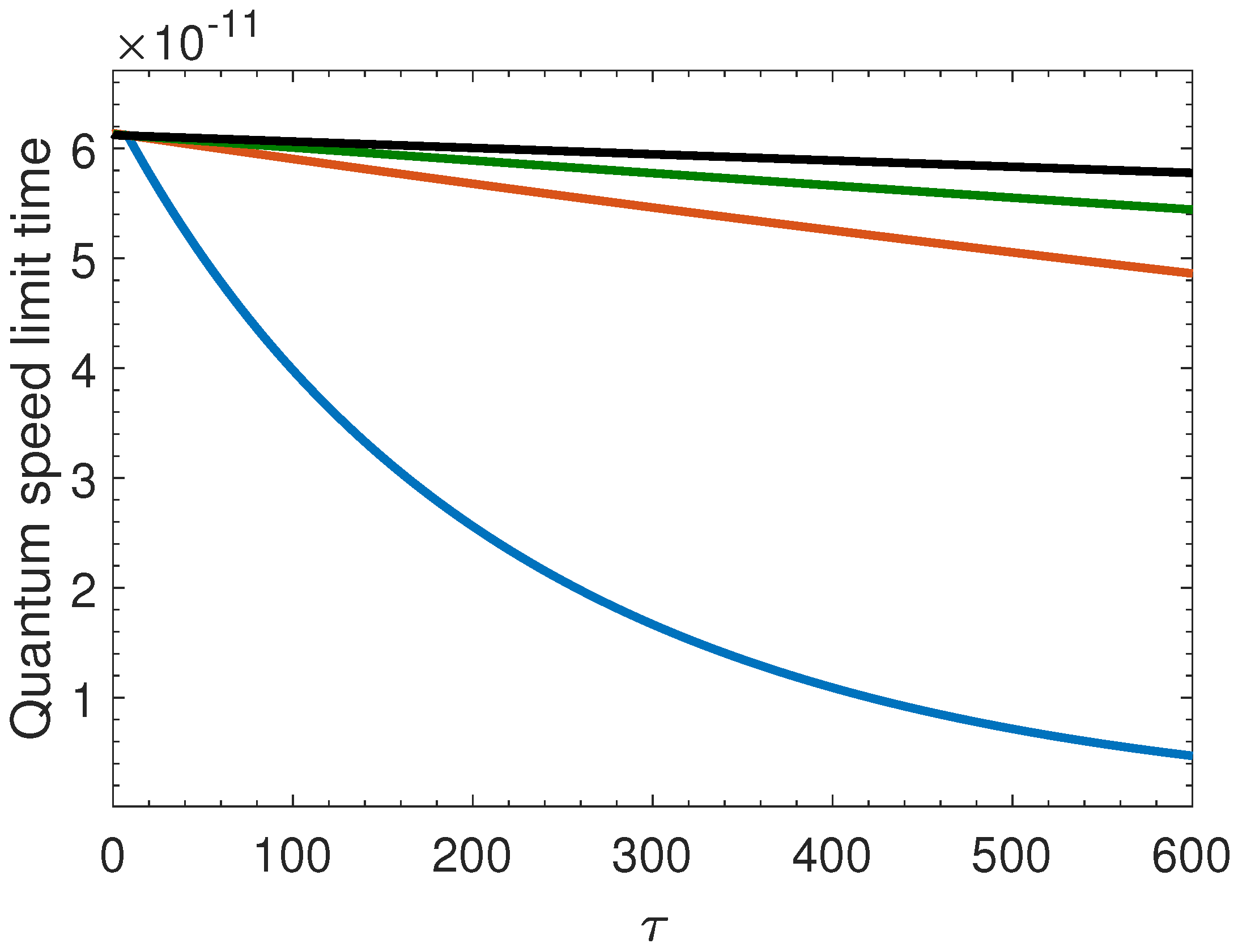
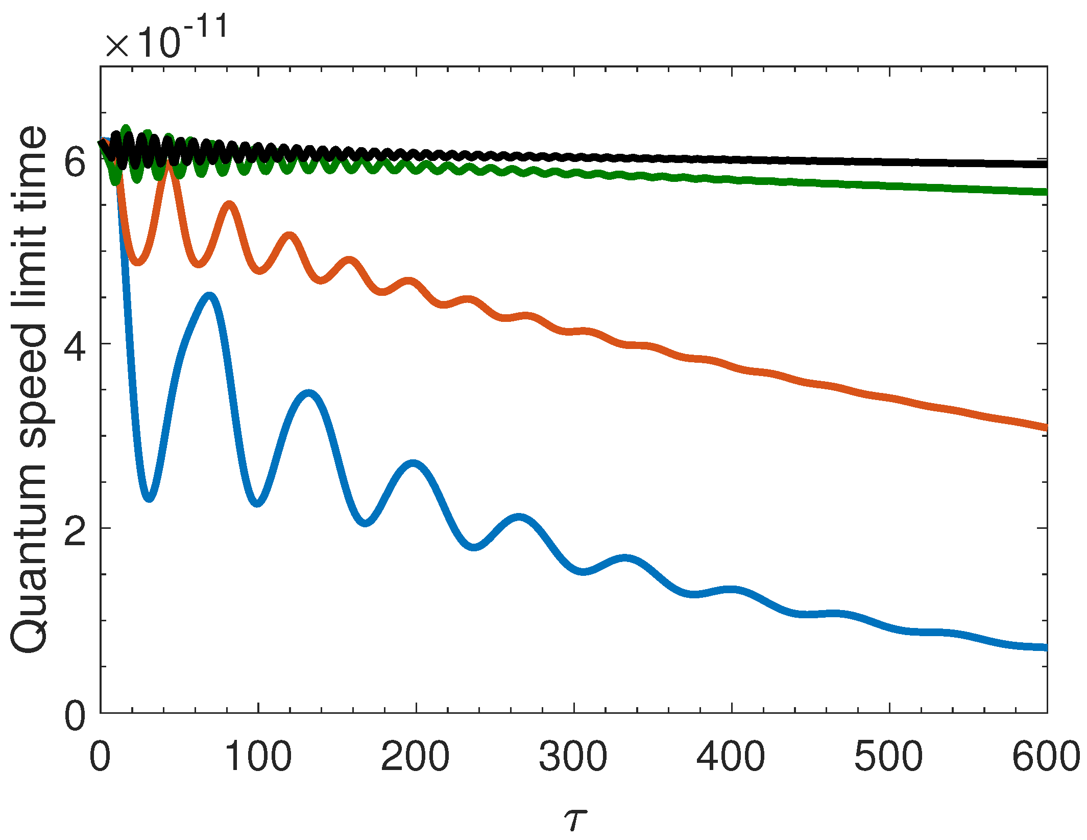
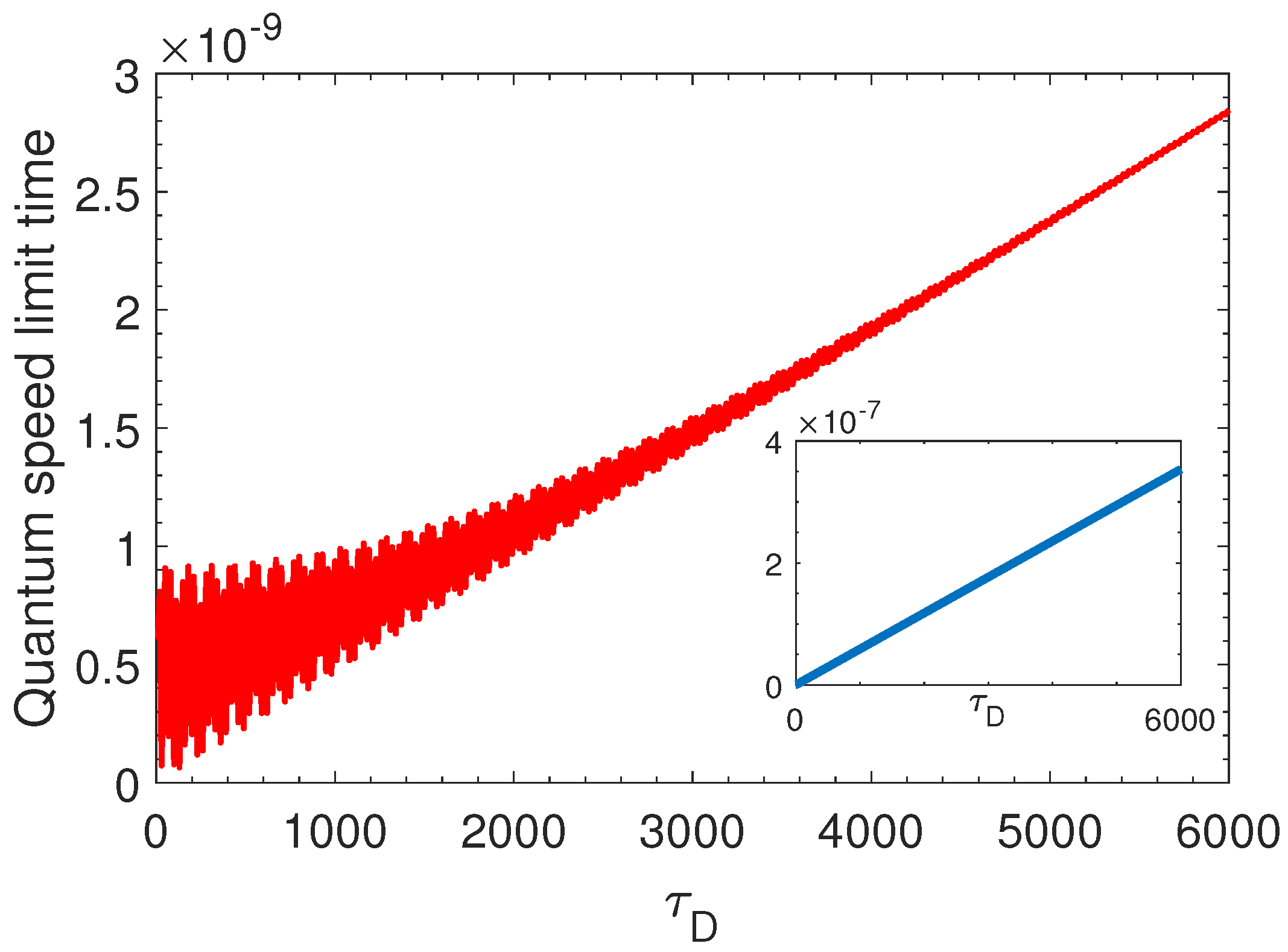
In this section, we first review one of the comprehensive criteria for determining the QSL time for open quantum systems [28], and then the QSL time is studied for a moving qubit inside a leaky cavity. The dynamics of an open quantum system are described via the following master equation

$${\dot{\rho }}_t={\mathcal{L}}_t\left({\rho }_t\right),$$

(22)

where ${\rho }_t$ is the evolved state of the system at time t and ${\mathcal{L}}_t$ (the Liouvillian super-operator) is the linear generator of quantum evolution that preserves the algebraic properties of the density matrix (trace, positivity, and Hermiticity) [60]. It has been demonstrated that time-dependent generators of quantum evolution ${\mathcal{L}}_t$ can lead to memory effects; see, for example, Refs. [61,62,63,64,65]. QSL time is defined as the shortest time required to evolve from ${\rho }_{\tau }$ to ${\rho }_{\tau +{\tau }_D}$, where $\tau$ is the initial time and ${\tau }_D$ is the driving time. Indeed, ${\tau }_D$ is the time taken for the system to reach a desired state ${\rho }_{\tau +{\tau }_D}$ from an initial state ${\rho }_{\tau }$. If the QSL time is equal to the driving time, the evolution of the quantum system cannot accelerate, while if the QSL time is smaller than the driving time, there is a potential for the evolution of the quantum system to accelerate. In Ref. [28], the authors have used relative purity to calculate the QSL time for open quantum systems. They have shown that the relative purity between the state at initial time $\tau$ and the target state at time $\tau +{\tau }_D$ can be written as

$$\mathcal{F}\left(\tau +{\tau }_D\right)=\frac{tr\left({\rho }_{\tau }{\rho }_{\tau +{\tau }_D}\right)}{tr\left({\rho }_{\tau }^2\right)}.$$

(23)

By following the method outlined in Ref. [28], the ML bound for QSL time can be obtained as follows:

$${\tau }_{QSL}^{\mathrm{ML}}=\frac{\left|\mathcal{F}\left(\tau +{\tau }_D\right)-1\right|tr\left({\rho }_{\tau }^2\right)}{\overline{{\sum }_{i=1}^n{\kappa }_i{\varrho }_i}},$$

(24)

where ${\varrho }_i$ and ${\kappa }_i$ are the singular values of ${\rho }_{\tau }$ and ${\mathcal{L}}_t\left({\rho }_t\right)$, respectively, and $\overline{\square }=\frac{1}{{\tau }_D}{\int }_{\tau }^{\tau +{\tau }_D}\square dt$. The MT bound of QSL time can also be obtained similarly as follows:

$${\tau }_{QSL}^{\mathrm{MT}}=\frac{\left|\mathcal{F}\left(\tau +{\tau }_D\right)-1\right|tr\left({\rho }_{\tau }^2\right)}{\overline{\sqrt{{\sum }_{i=1}^n{\kappa }_i^2}}}.$$

(25)

By merging these two bounds for QSL time, a comprehensive bound can be achieved as follows:

$${\tau }_{QSL}=max\left\{\frac{1}{\overline{{\sum }_{i=1}^n{\kappa }_i{\varrho }_i}},\frac{1}{\overline{\sqrt{{\sum }_{i=1}^n{\kappa }_i^2}}}\right\}\times \left|\mathcal{F}\left(\tau +{\tau }_D\right)-1\right|tr\left({\rho }_{\tau }^2\right).$$

(26)

It has also been shown that the ML bound in Equation (24) is tighter than the MT bound in Equation (25) [28]. The QSL time is inversely related to the speed of evolution in such a way that with increasing QSL time, the speed of evolution decreases and vice versa. In this work, we consider the maximally coherent initial state. This means that we put $c_1=c_2=1/\sqrt{2}$ in Equation (9). Therefore, the evolved density matrix has the following form

$$\rho \left(t\right)=\frac{1}{2}\left(\begin{array}{cc}{\left|A\left(t\right)\right|}^2& A\left(t\right)\\ A^{*}\left(t\right)& 2-{\left|A\left(t\right)\right|}^2\end{array}\right).$$

(27)

Let us calculate the singular values of ${\rho }_{\tau }$ and ${\mathcal{L}}_t\left({\rho }_t\right)$, respectively. For ${\rho }_{\tau }$, the singular values are

$${\varrho }_{1,2}=\frac{1}{2}\mp \frac{1}{2}\sqrt{{\left|A\left(\tau \right)\right|}^4-{\left|A\left(\tau \right)\right|}^2+1}.$$

(28)

The singular values ${\kappa }_i$ of ${\mathcal{L}}_t\left({\rho }_t\right)$ can be obtained as

$${\kappa }_1={\kappa }_2=\frac{1}{2}\sqrt{{\omega }_0^2{\left|A\left(t\right)\right|}^2+{\left|\dot{A}\left(t\right)\right|}^2-i{\omega }_{0}A\left(t\right)\dot{A}{\left(t\right)}^{*}+i{\omega }_{0}A{\left(t\right)}^{*}\dot{A}\left(t\right)+4A{\left(t\right)}^2\dot{A}{\left(t\right)}^2}.$$

(29)

Finally, the QSL time for the qubit to evolve from ${\rho }_{\tau }$ to ${\rho }_{\tau +{\tau }_D}$ can be obtained as

$${\tau }_{QSL}^{AD}=\frac{\left|\mathcal{F}\left(\tau +{\tau }_D\right)-1\right|tr\left({\rho }_{\tau }^2\right)}{\frac{1}{{\tau }_D}{\int }_{\tau }^{\tau +{\tau }_D}\left({\varrho }_1{\kappa }_1+{\varrho }_2{\kappa }_2\right)dt},$$

(30)

where

$$\begin{array}{cc}\hfill \left|\mathcal{F}\left(\tau +{\tau }_D\right)-1\right|tr\left({\rho }_{\tau }^2\right)& ={|-2|A\left(\tau \right)|}^4+{2\left(\right|A\left(\tau \right)|}^2-1\left)\right|A(\tau +{\tau }_D){|}^2\hfill \\ \hfill & +e^{-ik{\omega }_0}A(\tau +{\tau }_D)A{\left(\tau \right)}^{*}+e^{ik{\omega }_0}A{(\tau +{\tau }_D)}^{*}A\left(\tau \right)|.\hfill \end{array}$$

(31)

In Figure 2, the QSL time (30) is plotted in terms of initial time $\tau$ for weak coupling regime ($\gamma <\lambda /2$). Also, different values of the velocity of moving qubit $\beta$ have been considered. In a weak coupling regime, the dynamics is Markovian. As can be seen, the QSL time increases by enhancing the velocity of the moving qubit. It can also be seen that with increasing qubit velocity, QSL time almost reaches a constant value, and it leads to a uniform speed for the dynamics. In fact, by increasing the velocity of the qubit inside the leaky cavity, coherence is protected, so the speed of evolution decreases. It can be stated that by increasing the qubit velocity inside the leaky cavity, the single-qubit system will be more stable, and the process of losing coherence will be slower.

In Figure 3, the QSL time is plotted as a function of $\tau$ for a strong coupling regime ($\gamma >\lambda /2$). As mentioned before, in a strong coupling regime, the dynamics are non-Markovian, and information flows back from the environment to the system. In this figure, the QSL time is plotted for different values of the velocity of the moving qubit $\beta$. As can be seen, the QSL time has an oscillating behavior and decreases for small values of the velocity of the qubit. It is also observed that the QSL time grows with increasing the velocity of the qubit inside the leaky cavity. One can also be seen that with increasing qubit speed, QSL time almost reaches a constant value and, therefore, leads to a uniform evolution speed for the mentioned open system.

In Figure 4, we present the QSL time versus the driving time ${\tau }_D$. In the Markovian regime, we obtain a linear relation between the QSL time and ${\tau }_D$, which was an anticipated effect for the weak coupling scenario. However, when we shift to the strong coupling regime, we observe oscillations that are visible proof of non-Markovianity affecting the dynamics.

Finally, we illustrate the QSL time versus the environmental parameter $\lambda /\gamma$ and some fixed values in Figure 5. As mentioned before, for our cavity model, the dynamic is non-Markovian when $\lambda /\gamma <2$ and we have a strong coupling regime. Therefore, it can be said that the evolution moves towards being Markovian, and the QSL time increases with increasing $\lambda /\gamma$. Considering the inverse relationship between the QSL time and the speed of evolution, it can be said that with the increase of $\lambda /\gamma$, the evolution will become Markovian, and the speed of evolution will decrease, which is comparable to the results obtained in Ref. [66].

4. Discussion

The ability to determine the QSL time implies better controllability of open quantum systems [67,68,69,70,71]. By scrupulously manipulating the parameters, i.e., atom-photon coupling constant and qubit velocity, we can transfer an arbitrary initial state into the target one within a designated period of time. This can be considered environment-induced engineering of quantum states, which results in following a predetermined trajectory in the state set. On the other hand, for a given environment setting, one can predict the behavior of a two-level system in the optical cavity. The interactions between an atom and photons are a form of decoherence that affects the initially encoded qubit. However, we can track the qubit in the time domain and steer the pace of its evolution by regulating the velocity. As it is demonstrated, by increasing the velocity, we can slow down the evolution, which partially protects the qubit from decoherence.

Finally, let us discuss the significance of the results in reference to quantum state tomography (QST). There are numerous frameworks of state reconstruction that benefit from applying knowledge about dynamics; see, for example, Refs. [72,73]. Such approaches allow one to generate a time-dependent measurement record, which can be either discrete [74] or continuous [75]. However, the main challenge related to dynamical QST frameworks is associated with the difficulty in manipulating time in microstructures. Therefore, the results presented in this manuscript, which precisely quantify the QSL time for various settings, give hope for constructing enhanced QST models for the tomography of qubits trapped in an optical cavity. In such models, it will be necessary to take into account different sources of errors associated with optical cavities, such as the thermal noise [76,77].

5. Conclusions

In the quantum world, we are mostly dealing with open quantum systems. Due to the importance of open quantum systems, the study of the dynamics and properties of these systems is of particular interest. One of the features that can be considered in both closed and open quantum systems is the QSL time. In this work, a framework is considered as an open quantum system in which a single qubit moves inside a leaky cavity. The motivation for choosing such a structure is that in this model, as a result of the movement of a single qubit with high speed, the degree of coherence of the initial state remains more stable during the evolution. In this structure, both strong coupling and weak coupling of the system with cavity modes were considered. In a weak coupling regime, the dynamics is Markovian (memory-less), which means that information is leaked from the system to the environment monotonically, and there is no flow back of information. Conversely, in a strong coupling regime, the dynamic is non-Markovian (with memory effects), and information flows back from the environment to the system during the evolution.

In this work, the QSL time was studied for the mentioned model, i.e., the moving qubit inside a leaky cavity. In the case of a weak coupling regime, it was observed that the QSL time decreases monotonically with increasing initial time $\tau$. It was also observed that with the increasing velocity of the qubit inside the leaky cavity, the QSL time increases. Due to the inverse relationship between QSL time and speed of the evolution, it can be said that by increasing the qubit velocity inside the leaky cavity, the speed of evolution decreases and the system is more stable. Of course, such a result was predictable due to the direct relation between the coherence of the initial state and the QSL time. In the case of a strong coupling regime, it was observed that the QSL time decreases with an oscillating behavior. It was also observed that the QSL time increases when boosting the velocity of the qubit inside a leaky cavity. In summary, one can conclude that in the mentioned model, for both strong and weak coupling regimes, increasing the velocity of the qubit inside a leaky cavity leads to an increase in the QSL time and slowing down the evolution.

References

1. Bekenstein, J.D. Energy cost of information transfer. Phys. Rev. Lett. 1981, 46, 623. [Google Scholar] [CrossRef]
2. Giovanetti, V.; Lloyd, S.; Maccone, L. Advances in quantum metrology. Nat. Photonics 2011, 5, 222. [Google Scholar] [CrossRef] [Green Version]
3. Lloyd, S. Computational capacity of the Universe. Phys. Rev. Lett. 2002, 88, 237901. [Google Scholar] [CrossRef] [PubMed] [Green Version]
4. Caneva, T.; Murphy, M.; Calarco, T.; Fazio, R.; Montangero, S.; Giovannetti, V.; Santoro, G.E. Optimal control at the quantum speed limit. Phys. Rev. Lett. 2009, 103, 240501. [Google Scholar] [CrossRef] [PubMed]
5. Uhlmann, A. An energy dispersion estimate. Phys. Lett. A 1992, 161, 329. [Google Scholar] [CrossRef]
6. Pfeifer, P. How fast can a quantum state change with time? Phys. Rev. Lett. 1993, 70, 3365. [Google Scholar] [CrossRef]
7. Giovannetti, V.; Lloyd, S.; Maccone, L. Quantum limits to dynamical evolution. Phys. Rev. A 2003, 67, 052109. [Google Scholar] [CrossRef] [Green Version]
8. Pfeifer, P.; Fröhlich, J. Generalized time-energy uncertainty relations and bounds on lifetimes of resonances. Rev. Mod. Phys. 1995, 67, 759. [Google Scholar] [CrossRef] [Green Version]
9. Chau, H.F. Tight upper bound of the maximum speed of evolution of a quantum state. Phys. Rev. A 2010, 81, 062133. [Google Scholar] [CrossRef] [Green Version]
10. Deffner, S.; Lutz, E. Energy–time uncertainty relation for driven quantum systems. J. Phys. A Math. Theor. 2013, 46, 335302. [Google Scholar] [CrossRef]
11. Mandelstam, L.; Tamm, I. Quantum speed limits: From Heisenberg’s uncertainty principle to optimal quantum control. J. Phys. (USSR) 1945, 9, 249. [Google Scholar]
12. Margolus, N.; Levitin, L.B. The maximum speed of dynamical evolution. Physica D 1998, 120, 188. [Google Scholar] [CrossRef] [Green Version]
13. Levitin, L.B.; Toffoli, T. Fundamental limit on the rate of quantum dynamics: The unified bound is tight. Phys. Rev. Lett. 2009, 103, 160502. [Google Scholar] [CrossRef] [PubMed] [Green Version]
14. Davies, E.B. Quantum Theory of Open Systems; Academic Press: London, UK, 1976. [Google Scholar]
15. Alicki, R.; Lendi, K. Quantum Dynamical Semigroups and Applications; Springer: Berlin, Germany, 1987. [Google Scholar]
16. Breuer, H.P.; Petruccione, F. The Theory of Open Quantum Systems; Oxford University Press: Oxford, UK, 2002. [Google Scholar]
17. Fogarty, T.; Deffner, S.; Busch, T.; Campbell, S. Orthogonality catastrophe as a consequence of the quantum speed limit. Phys. Rev. Lett. 2020, 124, 110601. [Google Scholar] [CrossRef] [PubMed] [Green Version]
18. Puebla, R.; Deffner, S.; Campbell, S. Kibble-Zurek scaling in quantum speed limits for shortcuts to adiabaticity. Phys. Rev. Res. 2020, 2, 032020. [Google Scholar] [CrossRef]
19. Poggi, P.M. Análisis de cotas inferiores para tiempos de control y su relación con el límite de velocidades cuántico. Anales AFA 2020, 31, 29. [Google Scholar] [CrossRef] [Green Version]
20. Campaioli, F.; Sloan, W.; Modi, K.; Pollock, F.A. Algorithm for solving unconstrained unitary quantum brachistochrone problems. Phys. Rev. A 2019, 100, 062328. [Google Scholar] [CrossRef] [Green Version]
21. Pires, D.P.; Cianciaruso, M.; Celeri, L.C.; Adesso, G.; Soares-Pinto, D.O. Generalized geometric quantum speed limits. Phys. Rev. X 2016, 6, 021031. [Google Scholar] [CrossRef] [Green Version]
22. Taddei, M.M.; Escher, B.M.; Davidovich, L.; De Matos Filho, R.L. Quantum speed limit for physical processes. Phys. Rev. Lett. 2013, 110, 050402. [Google Scholar] [CrossRef]
23. del Campo, A.; Egusquiza, I.L.; Plenio, M.B.; Huelga, S.F. Quantum speed limits in open system dynamics. Phys. Rev. Lett. 2013, 110, 050403. [Google Scholar] [CrossRef] [Green Version]
24. Deffner, S.; Lutz, E. Quantum speed limit for non-Markovian dynamics. Phys. Rev. Lett. 2013, 111, 010402. [Google Scholar] [CrossRef]
25. Sun, Z.; Liu, J.; Ma, J.; Wang, X. Quantum speed limits in open systems: Non-Markovian dynamics without rotating-wave approximation. Sci. Rep. 2015, 5, 8444. [Google Scholar] [CrossRef] [Green Version]
26. Mondal, D.; Datta, C.; Sazim, S. Quantum coherence sets the quantum speed limit for mixed states. Phys. Lett. A 2016, 380, 689. [Google Scholar] [CrossRef] [Green Version]
27. Jones, P.J.; Kok, P. Geometric derivation of the quantum speed limit. Phys. Rev. A 2010, 82, 022107. [Google Scholar] [CrossRef] [Green Version]
28. Zhang, Y.J.; Han, W.; Xia, Y.J.; Cao, J.P.; Fan, H. Quantum speed limit for arbitrary initial states. Sci. Rep. 2014, 4, 4890. [Google Scholar] [CrossRef] [PubMed] [Green Version]
29. Mirkin, N.; Toscano, F.; Wisniacki, D.A. Quantum-speed-limit bounds in an open quantum evolution. Phys. Rev. A 2016, 94, 052125. [Google Scholar] [CrossRef] [Green Version]
30. Uzdin, R.; Kosloff, R. Speed limits in Liouville space for open quantum systems. EPL 2016, 115, 40003. [Google Scholar] [CrossRef] [Green Version]
31. Zhang, L.; Sun, Y.; Luo, S. Quantum speed limit for qubit systems: Exact results. Phys. Lett. A 2018, 382, 2599. [Google Scholar] [CrossRef]
32. Teittinen, J.; Lyyra, H.; Maniscalco, S. There is no general connection between the quantum speed limit and non-Markovianity. New J. Phys. 2019, 21, 123041. [Google Scholar] [CrossRef]
33. Ektesabi, A.; Behzadi, N.; Faizi, E. Improved bound for quantum-speed-limit time in open quantum systems by introducing an alternative fidelity. Phys. Rev. A 2017, 95, 022115. [Google Scholar] [CrossRef] [Green Version]
34. Cai, X.; Zheng, Y. Quantum dynamical speedup in a nonequilibrium environment. Phys. Rev. A 2017, 95, 052104. [Google Scholar] [CrossRef]
35. Deffner, S. Geometric quantum speed limits: A case for Wigner phase space. New J. Phys. 2017, 19, 103018. [Google Scholar] [CrossRef]
36. Wu, S.X.; Yu, C.S. Quantum speed limit for a mixed initial state. Phys. Rev. A 2018, 98, 042132. [Google Scholar] [CrossRef] [Green Version]
37. Funo, K.; Shiraishi, N.; Saito, K. Speed limit for open quantum systems. New J. Phys. 2019, 21, 013006. [Google Scholar] [CrossRef]
38. Brody, D.C.; Longstaff, B. Evolution speed of open quantum dynamics. Phys. Rev. Res. 2019, 1, 033127. [Google Scholar] [CrossRef] [Green Version]
39. Campaioli, F.; Pollock, F.A.; Modi, K. Tight, robust, and feasible quantum speed limits for open dynamics. Quantum 2019, 3, 168. [Google Scholar] [CrossRef] [Green Version]
40. Van Vu, T.; Hasegawa, Y. Geometrical bounds of the irreversibility in Markovian systems. Phys. Rev. Lett. 2021, 126, 010601. [Google Scholar] [CrossRef]
41. Campaioli, F.; Yu, C.S.; Pollock, F.A.; Modi, K. Resource speed limits: Maximal rate of resource variation. New J. Phys. 2022, 24, 065001. [Google Scholar] [CrossRef]
42. Bagheri Harouni, M. Quantum speed limit time and entanglement in a non-Markovian evolution of spin qubits of coupled quantum dots. Chin. Phys. B 2020, 29, 124203. [Google Scholar] [CrossRef]
43. Bagheri Harouni, M. Influences of spin-orbit interaction on quantum speed limit and entanglement of spin qubits in coupled quantum dots. Chin. Phys. B 2021, 30, 090301. [Google Scholar] [CrossRef]
44. Dehdashti, S.; Yasar, F.; Bagheri Harouni, M.; Mahdifar, A.; Mirza, B. Quantum speed limit in the thermal spin-boson system with and without tunneling term. Quant. Inf. Process. 2020, 19, 308. [Google Scholar] [CrossRef]
45. Awasthi, N.; Joshi, D.K.; Sachdev, S. Variation of quantum speed limit under Markovian and non-Markovian noisy environment. Laser Phys. Lett. 2022, 19, 035201. [Google Scholar] [CrossRef]
46. Awasthi, N.; Joshi, D.K.; Sachdev, S. Dynamics of quantum speed limit time for correlated and uncorrelated noise channels. Int. J. Theor. Phys. 2022, 61, 123. [Google Scholar] [CrossRef]
47. Lan, K.; Xie, S.; Cai, X. Geometric quantum speed limits for Markovian dynamics in open quantum systems. New J. Phys. 2022, 24, 055003. [Google Scholar] [CrossRef]
48. Haseli, S.; Salimi, S.; Dolatkhah, H.; Khorashad, A.S. Quantum speed limit time in the presence of disturbance. Mod. Phys. Lett. A 2021, 36, 2150009. [Google Scholar] [CrossRef]
49. Mortezapour, A.; Borji, M.A.; Park, D.; Franco, R.L. Non-Markovianity and coherence of a moving qubit inside a leaky cavity. Open Syst. Inf. Dyn. 2017, 24, 1740006. [Google Scholar] [CrossRef] [Green Version]
50. Mortezapour, A.; Borji, M.A.; Franco, R.L. Protecting entanglement by adjusting the velocities of moving qubits inside non-Markovian environments. Laser Phys. Lett. 2017, 14, 055201. [Google Scholar] [CrossRef] [Green Version]
51. Calajo, G.; Rabl, P. Strong coupling between moving atoms and slow-light Cherenkov photons. Phys. Rev. A 2017, 95, 043824. [Google Scholar] [CrossRef] [Green Version]
52. Garcia, L.A.; Felicetti, S.; Rico, E.; Solano, E.; Sabin, C. Entanglement of superconducting qubits via acceleration radiation. Sci. Rep. 2017, 7, 657. [Google Scholar] [CrossRef] [Green Version]
53. Felicetti, S.; Sabin, C.; Fuentes, I.; Lamata, L.; Romero, G.; Solano, E. Relativistic motion with superconducting qubits. Phys. Rev. B 2015, 92, 064501. [Google Scholar] [CrossRef] [Green Version]
54. Moustos, D.; Anastopoulos, C. Non-Markovian time evolution of an accelerated qubit. Phys. Rev. D 2017, 95, 025020. [Google Scholar] [CrossRef]
55. Lang, R.; Scully, M.O.; Lamb, W.E. Why is the laser line so narrow? A theory of single-quasimode laser operation. Phys. Rev. A 1973, 7, 1788. [Google Scholar] [CrossRef]
56. Gea-Banacloche, J.; Lu, N.; Pedrotti, L.M.; Prasad, S.; Scully, M.O.; Wodkiewicz, K. Treatment of the spectrum of squeezing based on the modes of the universe. I. Theory and a physical picture. Phys. Rev. A 1990, 41, 369. [Google Scholar] [CrossRef] [PubMed]
57. Leonardi, C.; Vaglica, A. Non-markovian dynamics and spectrum of a moving atom strongly coupled to the field in a damped cavity. Opt. Commun. 1993, 97, 130. [Google Scholar] [CrossRef]
58. Franco, R.L.; Bellomo, B.; Maniscalco, S.; Compagno, G. Dynamics of quantum correlations in two-qubit systems within non-Markovian environments. Int. J. Mod. Phys. B 2013, 27, 1345053. [Google Scholar] [CrossRef] [Green Version]
59. Bellomo, B.; Franco, R.L.; Compagno, G. Non-Markovian effects on the dynamics of entanglement. Phys. Rev. Lett. 2007, 99, 160502. [Google Scholar] [CrossRef] [Green Version]
60. Rivas, A.; Huelga, S.F. Open Quantum Systems; Springer: Berlin, Germany, 2012. [Google Scholar]
61. Daffer, S.; Wodkiewicz, K.; Cresser, J.D.; Mclver, J.K. Depolarizing channel as a completely positive map with memory. Phys. Rev. A 2004, 70, 010304(R). [Google Scholar] [CrossRef] [Green Version]
62. Breuer, H.P.; Laine, E.M.; Piilo, J.; Vacchini, B. Colloquium: Non-Markovian dynamics in open quantum systems. Rev. Mod. Phys. 2016, 88, 021002. [Google Scholar] [CrossRef] [Green Version]
63. Czerwinski, A. Dynamics of open quantum systems—Markovian semigroups and beyond. Symmetry 2022, 14, 1752. [Google Scholar] [CrossRef]
64. Czerwinski, A. Entanglement dynamics governed by time-dependent quantum generators. Axioms 2022, 11, 589. [Google Scholar] [CrossRef]
65. Benabdallah, F.; Rahman, A.U.; Haddadi, S.; Daoud, M. Long-time protection of thermal correlations in a hybrid-spin system under random telegraph noise. Phys. Rev. E 2022, 106, 034122. [Google Scholar] [CrossRef] [PubMed]
66. Ahansaz, B.; Ektesabi, A. Quantum speedup, non-Markovianity and formation of bound state. Sci. Rep. 2019, 9, 14946. [Google Scholar] [CrossRef] [PubMed] [Green Version]
67. Schirmer, S.G.; Fu, H.; Solomon, A.I. Complete controllability of quantum systems. Phys. Rev. A 2001, 63, 063410. [Google Scholar] [CrossRef] [Green Version]
68. Wu, S.L.; Ma, W. Trajectory tracking for non-Markovian quantum systems. Phys. Rev. A 2022, 105, 012204. [Google Scholar] [CrossRef]
69. Song, Y.J.; Kuang, L.M. Controlling decoherence speed limit of a single impurity atom in a Bose–Einstein-condensate reservoir. Ann. Phys. (Berlin) 2019, 531, 1800423. [Google Scholar] [CrossRef] [Green Version]
70. Song, Y.J.; Tan, Q.S.; Kuang, L.M. Control quantum evolution speed of a single dephasing qubit for arbitrary initial states via periodic dynamical decoupling pulses. Sci. Rep. 2017, 7, 43654. [Google Scholar] [CrossRef] [Green Version]
71. Song, Y.J.; Kuang, L.M.; Tan, Q.S. Quantum speedup of uncoupled multiqubit open system via dynamical decoupling pulses. Quant. Inf. Process. 2016, 15, 2325. [Google Scholar] [CrossRef]
72. Silberfarb, A.; Jessen, P.S.; Deutsch, I.H. Quantum state reconstruction via continuous measurement. Phys. Rev. Lett. 2005, 95, 030402. [Google Scholar] [CrossRef] [Green Version]
73. Merkel, S.T.; Riofrío, C.A.; Flammia, S.T.; Deutsch, I.H. Random unitary maps for quantum state reconstruction. Phys. Rev. A 2010, 81, 032126. [Google Scholar] [CrossRef] [Green Version]
74. Czerwinski, A. Quantum state tomography with informationally complete POVMs generated in the time domain. Quantum Inf. Process. 2021, 20, 105. [Google Scholar] [CrossRef]
75. Czerwinski, A. Quantum tomography of entangled qubits by time-resolved single-photon counting with time-continuous measurements. Quantum Inf. Process. 2022, 21, 332. [Google Scholar] [CrossRef]
76. Numata, K.; Kemery, A.; Camp, J. Thermal-noise limit in the frequency stabilization of lasers with rigid cavities. Phys. Rev. Lett. 2004, 93, 250602. [Google Scholar] [CrossRef] [PubMed]
77. Xu, G.; Jiao, D.; Chen, L.; Zhang, L.; Dong, R.; Liu, T.; Wang, J. Thermal noise in cubic optical cavities. Photonics 2021, 8, 261. [Google Scholar] [CrossRef]
Figure 1. Schematic diagram of the model where the qubit moves inside a leaky cavity with a constant velocity of v.
Photonics 09 00875 g001
Figure 2. QSL time for moving qubit inside a leaky cavity versus initial time τ when λ = 3 γ , ω 0 = ω n = 1.53 GHz and τ D = 1 for different values of the velocity of the moving qubit. β = 15 × 10 9 (blue line), β = 50 × 10 9 (orange line), β = 70 × 10 9 (green line), β = 100 × 10 9 (black line).
Photonics 09 00875 g002
Figure 3. QSL time for moving qubit inside a leaky cavity versus initial time τ when λ = 0.01 γ , ω 0 = ω n = 1.53 GHz and τ D = 1 for different values of the velocity of the moving qubit. β = 0.05 × 10 9 (blue line), β = 0.1 × 10 9 (orange line), β = 0.3 × 10 9 (green line), and β = 0.5 × 10 9 (black line).
Photonics 09 00875 g003
Figure 4. QSL time for moving qubit inside a leaky cavity versus driving time τ D when ω 0 = ω n = 1.53 GHz, β = 1 × 10 9 , and τ = 0 for non-Markovian dynamics λ = 0.1 γ and Markovian dynamics (inset plot) λ = 3 γ .
Photonics 09 00875 g004
Figure 5. QSL time for moving qubit inside a leaky cavity versus λ / γ when ω 0 = ω n = 1.53 GHz, β = 1 × 10 9 , τ D = 600 , and τ = 0 .
Photonics 09 00875 g005
Publisher’s Note: MDPI stays neutral with regard to jurisdictional claims in published maps and institutional affiliations.