Fast Quantum State Reconstruction via Accelerated Non-Convex Programming

Abstract

We propose a new quantum state reconstruction method that combines ideas from compressed sensing, non-convex optimization, and acceleration methods. The algorithm, called Momentum-Inspired Factored Gradient Descent (MiFGD), extends the applicability of quantum tomography for larger systems. Despite being a non-convex method, MiFGD converges provably close to the true density matrix at an accelerated linear rate asymptotically in the absence of experimental and statistical noise, under common assumptions. With this manuscript, we present the method, prove its convergence property and provide the Frobenius norm bound guarantees with respect to the true density matrix. From a practical point of view, we benchmark the algorithm performance with respect to other existing methods, in both synthetic and real (noisy) experiments, performed on the IBM’s quantum processing unit. We find that the proposed algorithm performs orders of magnitude faster than the state-of-the-art approaches, with similar or better accuracy. In both synthetic and real experiments, we observed accurate and robust reconstruction, despite the presence of experimental and statistical noise in the tomographic data. Finally, we provide a ready-to-use code for state tomography of multi-qubit systems.

1. Introduction

Quantum tomography is one of the main procedures to identify the nature of imperfections and deviations in quantum processing unit (QPU) implementations [1,2]. Generally, quantum tomography is composed of two main parts: (i) measuring the quantum system, and (ii) analyzing the measurement data to obtain an estimate of the density matrix (in the case of state tomography [1]), or of the quantum process (in the case of process tomography [3]). In this manuscript, we focus on the state tomography.

Quantum tomography is generally considered as a non-scalable protocol [4], as the number of free parameters that define quantum states and processes scale exponentially with the number of subsystems. In particular, quantum state tomography (QST) suffers from two bottlenecks. The first concerns about the large amount of data one needs to collect to perform tomography; the second concerns about numerically searching in an exponentially increasing space for a density matrix that is consistent with the data.

There have been various approaches to improve the scalability of QST, in terms of the amount of data required [5,6,7]. To address the data collection bottleneck, prior information about the unknown quantum state is often assumed. For example, in compressed sensing QST [4,8], the density matrix of the quantum system is assumed to be low-rank. In neural network QST [9,10,11], the wave-functions are often assumed to be real and positive, confining the landscape of quantum states (To handle more complex wave-functions, neural network approaches require a proper re-parameterization of the Restricted Boltzmann machines [9]). The prior information considered in these cases is that they are characterized by structured quantum states [9] (Such assumptions are often the reason behind accurate solutions of neural network QST in high-dimensional spaces.) Ref. [9] considers also the case of a completely unstructured case and test the limitation of this technique, which does not perform as expected, due to lack of any exploitable structure). Similarly, in matrix-product-state tomography [12,13], one assumes that the quantum state can be represented with low bond-dimension matrix-product state.

To address the computational bottleneck, several works introduce sophisticated numerical methods to improve the efficiency of QST. In particular, variants of gradient-based convex solvers—e.g., [14,15,16,17]—have been tested on synthetic scenarios [17]. The problem is that, achieving these results often requires utilizing special-purpose hardwares, such as Graphics Processing Units (GPUs), on top of carefully designing a proper distributed system [18]. Thus, going beyond current capabilities requires novel methods that can efficiently search in the space of density matrices under more realistic scenarios. Importantly, such numerical methods should come with rigorous guarantees on their convergence and performance.

The setup we consider here is the estimation of an n-qubit state, under the prior assumption that the state is close to a pure state, and thus its density matrix is of low-rank. This assumption is justified by the state-of-the-art experiments, where the aim is to manipulate the pure states with unitary maps. From a theoretical perspective, the low-rank assumption implies that we can use compressed sensing techniques [19], which allow the recovery of the density matrix from relatively fewer measurement data [20,21].

Indeed, compressed sensing QST is widely used for estimating highly-pure quantum states; e.g., [4,22,23,24]. However, compressed sensing QST usually relies on convex optimization for the estimation [8], which limits the applicability to relatively small system sizes [4] (In particular, convex solvers over low-rank structures utilize the nuclear norm over $2^n\times 2^n$ matrices. This assumes calculating all $2^n$ eigenvalues of such matrices per iteration, which has cubic complexity $O\left({\left(2^n\right)}^3\right)$). On the other hand, non-convex optimization approaches could preform much faster than their convex counterparts [25]. Although non-convex optimization typically lacks convergence guarantees, it was recently shown that one can formulate the compressed sensing QST as a non-convex problem, and solve it with rigorous convergence guarantees (under certain but generic conditions), allowing the state estimation of larger system sizes [26].

Following the non-convex path, we introduce a new algorithm to the toolbox of QST—the Momentum-Inspired Factored Gradient Descent (MiFGD). Our approach combines the ideas from compressed sensing, non-convex optimization, and acceleration/momentum techniques to scale QST beyond the current capabilities. MiFGD includes acceleration motions per iteration, meaning that it uses two previous iterates to update the next estimate; see Section 2 for details. The intuition is that if the k-th and $(k-1)$-th estimates were pointing to the correct direction, then both information should be useful to determine the $(k+1)$-th estimate. Of course such approach requires an additional estimate to be stored—yet, we show both theoretically and experimentally that momentum results in faster estimation. We emphasize that the analysis becomes non-trivially challenging due to the inclusion of two previous iterates.

The contributions of the paper are summarized as follows:

(i)

We prove that the non-convex MiFGD algorithm asymptotically enjoys an accelerated linear convergence rate in terms of the iterate distance, in the noiseless measurement data case and under common assumptions.

(ii)

We provide QST results using the real measurement data from IBM’s quantum computers up to 8-qubits, contributing to recent efforts on testing QST algorithms in real quantum data [22]. Our synthetic examples scale up to 12-qubits effortlessly, leaving the space for an efficient and hardware-aware implementation open for future work.

(iii)

We show through extensive empirical evaluations that MiFGD allows faster estimation of quantum states compared to the state-of-the-art convex and non-convex algorithms, including recent deep learning approaches [9,10,11,27], even in the presence of statistical noise in the measurement data.

(iv)

We further increase the efficiency of MiFGD by extending its implementation to utilize parallel execution over the shared and distributed memory systems. We experimentally showcase the scalability of our approach, which is particularly critical for the estimation of larger quantum system.

(v)

We provide the implementation of our approach at https://github.com/gidiko/MiFGD (accessed on 18 January 2023), which is compatible with the open-source software Qiskit [28].

The rest of this manuscript is organized as follows. In Section 2, we set up the problem in detail, and present our proposed method: MiFGD. Then, we detail the experimental set up in Section 3, followed by the results in Section 4. Finally, we discuss related and future works with concluding remarks in Section 5.

2. Methods

2.1. Problem Setup

We consider the estimation of a low-rank density matrix ${\rho }^{\star }\in {\mathbb{C}}^{d\times d}$ on an n-qubit Hilbert space with dimension $d=2^n$, through the following ${\ell }_2$-norm reconstruction objective:

$$\begin{array}{cccc}\hfill & \underset{\rho \in {\mathbb{C}}^{d\times d}}{\min }\hfill & \hfill & f\left(\rho \right):=\frac{1}{2}{\parallel \mathcal{A}\left(\rho \right)-y\parallel }_2^2\hfill \\ \hfill & \mathrm{subject}\mathrm{to}\hfill & \hfill & \rho ⪰0,\mathtt{rank}\left(\rho \right)\le r.\hfill \end{array}$$

(1)

Here, $y\in {\mathbb{R}}^m$ is the measurement data (observations) (Specific description on how y is generated and what it represents will follow), and $\mathcal{A}(·):{\mathbb{C}}^{d\times d}\to {\mathbb{R}}^m$ is the linear sensing map, where $m\ll d^2$. The sensing map relates the density matrix ${\rho }^{\star }$ to (expected, noiseless) observations through the Born rule: ${\left(\mathcal{A}\left(\rho \right)\right)}_i=\mathtt{Tr}\left(A_i\rho \right)$, where ${\left\{A_i\right\}}_{i=1}^m\in {\mathbb{C}}^{d\times d}$ are matrices closely related to the measured observable or the POVM elements of appropriate dimensions.

The objective function in Equation (1) has two constraints: the positive semi-definite constraint: $\rho ⪰0,$ and the low-rank constraint: $\mathtt{rank}\left(\rho \right)\le r$. The former is a convex constraint, whereas the latter is a non-convex one, rendering Equation (1) to be a non-convex optimization problem (Convex optimization problem requires both the objective function as well as the constraints to be convex). Following compressed sensing QST results [8], the unit trace constraint $\mathtt{Tr}\left(\rho \right)=1$ (which should be satisfied by any density matrix by definition) can be disregarded, without affecting the precision of the final estimate.

A pivotal assumption to apply compressed sensing results is that the linear sensing map $\mathcal{A}$ should satisfy the restricted isometry property, which we recall below.

Definition 1 

(Restricted Isometry Property (RIP) [29]). A linear operator $\mathcal{A}:{\mathbb{C}}^{d\times d}\to {\mathbb{R}}^m$ satisfies the RIP on rank-r matrices with the RIP constant ${\delta }_r\in (0,1)$, if the following holds with high probability for any rank-r matrix $X\in {\mathbb{C}}^{d\times d}$:

$$\begin{array}{c}\hfill (1-{\delta }_r)·{\parallel X\parallel }_F^2\le \parallel \mathcal{A}\left(X\right){\parallel }_2^2\le (1+{\delta }_r)·{\parallel X\parallel }_F^2.\end{array}$$

(2)

Such maps (almost) preserve the Frobenius norm of low-rank matrices, and, as an extension, of low-rank Hermitian matrices. The intuition behind RIP is that the operator $\mathcal{A}(·)$ behaves almost as a bijection between the subspaces ${\mathbb{C}}^{d\times d}$ and ${\mathbb{R}}^m$ for low-rank matrices.

Following recent works [26], instead of solving Equation (1), we propose to solve a factorized version of it:

$$\underset{U\in {\mathbb{C}}^{d\times r}}{\min }\frac{1}{2}{\parallel \mathcal{A}\left(U{U}^{†}\right)-y\parallel }_2^2,$$

(3)

where $U^{†}\in {\mathbb{C}}^{r\times d}$ denotes the adjoint of U, and $\rho$ is re-parametrized with $\rho =U{U}^{†}$. The motivation for this reformulation is two-folds. First, by representing the $d\times d$ dimensional density matrix $\rho$ with (the outer product of) its $d\times r$ dimensional low-rank factors U, the search space for the density matrix (that is consistent with the measurement data) significantly reduces, given that $r\ll d$. Second, via the reformulation $\rho =U{U}^{†},$ both the PSD constraint and the low-rank constraint are automatically satisfied, transforming the constrained optimization problem in Equation (1) to the unconstrained optimization problem in Equation (3). An important implication is that, to solve Equation (3), one can bypass the projection step onto the PSD and low-rank subspace, which requires a sigular value decomposition (SVD) of the estimate of the density matrix $\rho$ on every iteration. This is prohibitively expensive when the dimension $d=2^n$ is large, which is the case for even moderate number of qubits n. As such, working in the factored space was shown to improve time and space complexities [26,30,31,32,33,34].

A common approach to solve a factored objective as in Equation (3) is to use gradient descent [35] on the parameter U, with iterates as follows (We assume the case where $\nabla f(·)=\nabla f{(·)}^{†}$. If this does not hold, the theory still holds by carrying around $\nabla f(·)+\nabla f{(·)}^{†}$ instead of just $\nabla f(·)$, after proper scaling):

$$\begin{array}{cc}\hfill U_{k+1}& =U_k-\eta \nabla f\left(U_k{U}_k^{†}\right)·U_k\hfill \end{array}$$

(4)

$$\begin{array}{cc}\hfill & =U_k-\eta {\mathcal{A}}^{†}\left(\mathcal{A}\left(U_k{U}_k^{†}\right)-y\right)·U_k.\hfill \end{array}$$

(5)

Here, $U_k\in {\mathbb{C}}^{d\times r}$ is the k-th iterate, and the operator ${\mathcal{A}}^{†}:{\mathbb{R}}^m\to {\mathbb{C}}^{d\times d}$ is the adjoint of $\mathcal{A}$, defined as ${\mathcal{A}}^{†}\left(x\right)={\sum }_{i=1}^m{x}_i{A}_i$, for $x\in {\mathbb{R}}^m$. The hyperparameter $\eta >0$ is the step size. This algorithm has been studied in [25,32,34,36,37,38]. We will refer to the above iteration as the factored gradient descent (FGD) algorithm, as in [30]. In what follows, we will introduce our proposed method, the MiFGD algorithm: momentum-inspired factored gradient descent.

2.2. The MiFGD Algorithm

The MiFGD algorithm is a two-step variant of FGD, which iterates as follows:

$$\begin{array}{cc}\hfill U_{k+1}& =Z_k-\eta {\mathcal{A}}^{†}\left(\mathcal{A}\left(Z_k{Z}_k^{†}\right)-y\right)·Z_k,\hfill \end{array}$$

(6)

$$\begin{array}{cc}\hfill Z_{k+1}& =U_{k+1}+\mu \left(U_{k+1}-U_k\right).\hfill \end{array}$$

(7)

Here, $Z_k\in {\mathbb{C}}^{d\times r}$ is a rectangular matrix (with the same dimension as $U_k$) that accumulates the “momentum” of the iterates $U_k$ [39]. $\mu$ is the momentum parameter that weighs the amount of mixture of the previous estimate $U_k$ and the current $U_{k+1}$ to generate $Z_{k+1}$. The above iteration is an adaptation of Nesterov’s accelerated first-order method for convex problems [40]. We borrow this momentum formulation, and study how the choice of the momentum parameter $\mu$ affects the overall performance in non-convex problem formulations, such as Equation (3). We note that the theory and algorithmic configurations in [40] do not generalize to non-convex problems, which is one of the contributions of this work. Albeit being a non-convex problem, we show that MiFGD asymptotically converges at an accelerated linear rate around a neighborhood of the optimal value, akin to convex optimization results [40].

An important observation is that the factorization $\rho =U{U}^{†}$ is not unique. For instance, suppose that $U^{\star }$ is an optimal solution for Equation (3); then, for any rotation matrix $R\in {\mathbb{C}}^{r\times r}$ satisfying $R{R}^{†}=I$, the matrix $\widehat{U}=U^{\star }R$ is also optimal for Equation (3) (To see this, observe that ${\rho }^{\star }=U^{\star }{U}^{\star †}=U^{\star }I{U}^{\star †}=U^{\star }R{R}^{†}{U}^{\star †}=\widehat{U}{\widehat{U}}^{†}$). To resolve this ambiguity, we use the distance between a pair of matrices as the minimum distance ${\min }_{R\in \mathcal{O}}{∥U-U^{\star }R∥}_F$ up to rotations, where $\mathcal{O}=\{R\in {\mathbb{C}}^{r\times r}|R{R}^{†}=I\}$. In words, we want to track how close an estimate U is to $U^{\star }$, up to the minimizing rotation matrix.

Algorithm 1 contains the details of the MiFGD. As Problem (3) is non-convex, the initialization plays an important role in achieving global convergence. The initial point $U_0$ is either randomly initialized [36,41,42], or set according to Lemma 4 in [26]:

$$\begin{array}{c}\hfill {\rho }_0=U_0{U}_0^{†}={\mathrm{\Pi }}_{\mathcal{C}}\left(\frac{-1}{1+{\delta }_{2r}}·\nabla f\left(0\right)\right)=\frac{1}{1+{\delta }_{2r}}{\mathrm{\Pi }}_{\mathcal{C}}\left({\displaystyle \sum _{i=1}^m}{y}_i{A}_i\right),\end{array}$$

(8)

where ${\mathrm{\Pi }}_{\mathcal{C}}(·)$ is the projection onto the set of PSD matrices, ${\delta }_{2r}\in (0,1)$ is the RIP constant from Definition 1, and $\nabla f\left(0\right)$ is the gradient of $f(·)$ evaluated at all-zero matrix. Since computing the RIP constant is NP-hard, in practice we compute $U_0$ through ${\rho }_0=\frac{-1}{\widehat{L}}{\mathrm{\Pi }}_{\mathcal{C}}\left({\sum }_{i=1}^m{y}_i{A}_i\right)$, where $\widehat{L}\in (1,\raisebox{1ex}{$11$}\!\left/ \!\raisebox{-1ex}{$10$}\right.]$; see Theorem 1 below for details.

Algorithm 1 Momentum-Inspired Factored Gradient Descent (MiFGD).

Input:$\mathcal{A}$ (sensing map), y (measurement data), r (rank), and $\mu$ (momentum parameter). $•$ Set $U_0$ randomly or as in Equation (8). $•$ Set $Z_0=U_0$. $•$ Set $\eta$ as in Equation (9). for  $k=0,1,2,\dots$do    $U_{k+1}=Z_k-\eta {\mathcal{A}}^{†}\left(\mathcal{A}\left(Z_k{Z}_k^{†}\right)-y\right)·Z_k$    $Z_{k+1}=U_{k+1}+\mu \left(U_{k+1}-U_k\right)$ end for  Output: $\rho =U_{k+1}{U}_{k+1}^{†}$

Compared to randomly selecting $U_0$, the initialization scheme in Equation (8) involves a gradient and a top-r eigenvalue computations. Yet, Equation (8) provides a more informed initial point, as it is based on the data ${\{y_i,A_i\}}_{i=1}^m$, which could lead to convergence in fewer iterations in practice, and satisfies the initialization condition of Theorem 1 for small enough $\kappa$ (Based on our experiments, in practice, both initializations are applicable and useful).

For the step size $\eta$ in Algorithm 1, it is set to the following based on our theoretical analysis (c.f., Lemma A6):

$$\begin{array}{c}\hfill \eta =\frac{1}{4\left((1+{\delta }_{2r})\parallel Z_0{Z}_0^{†}{\parallel }_2+{\parallel {\mathcal{A}}^{†}\left(\mathcal{A}\left(Z_0{Z}_0^{†}\right)-y\right)\parallel }_2\right)},\end{array}$$

(9)

where $Z_0=U_0$. Similarly to the above, in practice we replace the RIP constant ${\delta }_{2r}$ with $\widehat{L}$. The step size $\eta$ remains constant at every iteration, and requires only two top-eigenvalue computations to obtain the spectral norms $\parallel Z_0{Z}_0^{†}{\parallel }_2$ and $\parallel {\mathcal{A}}^{†}\left(\mathcal{A}(Z_0{Z}_0^{†}-y\right){\parallel }_2$. These computations can be efficiently implemented by any off-the-shelf eigenvalue solver, such as the Power Method or the Lanczos method [43].

2.3. Theoretical Guarantees of the MiFGD Algorithm

We now present the formal convergence theorem, where under certain conditions, MiFGD asymptotically achieves an accelerated linear rate.

Theorem 1 

(Accelerated asymptotic convergence rate). Assume that $\mathcal{A}(·)$ satisfies the RIP in Definition 1 with the constant ${\delta }_{2r}\le \raisebox{1ex}{$1$}\!\left/ \!\raisebox{-1ex}{$10$}\right.$. Initialize $U_0=U_{-1}$ such that

$$\begin{array}{c}\hfill {\displaystyle \underset{R\in \mathcal{O}}{\min }}\parallel U_0-U^{\star }{R\parallel }_F={\displaystyle \underset{R\in \mathcal{O}}{\min }}{\parallel U_{-1}-U^{\star }R\parallel }_F\le \frac{\sqrt{{\sigma }_r\left({\rho }^{\star }\right)}}{{10}^3\sqrt{\kappa \tau \left({\rho }^{\star }\right)}},\end{array}$$

where $\kappa :=\frac{1+{\delta }_{2r}}{1-{\delta }_{2r}}$ is the (inverse) condition number of $\mathcal{A}(·)$, $\tau \left(\rho \right):=\frac{{\sigma }_1\left(\rho \right)}{{\sigma }_r\left(\rho \right)}$ is the condition number of ρ with $\mathit{rank}\left(\rho \right)=r$, and ${\sigma }_i\left(\rho \right)$ is the i-th singular value of ρ. Set the step size η such that

$$\begin{array}{c}\hfill \left[1-{\left(\frac{\sqrt{1+{\delta }_{2r}}-\sqrt{1-{\delta }_{2r}}}{(\sqrt{2}+1)\sqrt{1+{\delta }_{2r}}}\right)}^4\right]·\frac{10}{4{\sigma }_r\left({\rho }^{\star }\right)(1-{\delta }_{2r})}\le \eta \le \frac{10}{4{\sigma }_r\left({\rho }^{\star }\right)(1-{\delta }_{2r})},\end{array}$$

and the momentum parameter $\mu =\frac{{\epsilon }_{\mu }}{2·{10}^{3}r\tau \left({\rho }^{\star }\right)\sqrt{\kappa }},$ for user-defined ${\epsilon }_{\mu }\in (0,1]$. Then, for the (noiseless) measurement data $y=\mathcal{A}\left({\rho }^{\star }\right)$ with rank$\left({\rho }^{\star }\right)=r,$ the output of the MiFGD in Algorithm 1 satisfies the following: for any $ϵ>0$, there exist constants $C_{ϵ}$ and ${\tilde{C}}_{ϵ}$ such that, for all k,

$$\begin{array}{cc}\hfill & {\left({\displaystyle \underset{R\in \mathcal{O}}{\min }}\parallel U_{k+1}-U^{\star }{R\parallel }_F^2+{\displaystyle \underset{R\in \mathcal{O}}{\min }}{\parallel U_k-U^{\star }R\parallel }_F^2\right)}^{1/2}\hfill \\ \hfill & \le C_{ϵ}{\left(1-\sqrt{\frac{1-{\delta }_{2r}}{1+{\delta }_{2r}}}+ϵ\right)}^{k+1}{\displaystyle \underset{R\in \mathcal{O}}{\min }}{\parallel U_0-U^{\star }R\parallel }_F+\xi ·\mu ·{\sigma }_1{\left({\rho }^{\star }\right)}^{1/2}·r·{\tilde{C}}_{ϵ}\hfill \\ \hfill & \approx C_{ϵ}{\left(1-\sqrt{\frac{1-{\delta }_{2r}}{1+{\delta }_{2r}}}+ϵ\right)}^{k+1}{\displaystyle \underset{R\in \mathcal{O}}{\min }}{\parallel U_0-U^{\star }R\parallel }_F+O\left(\mu \right).\hfill \end{array}$$

(10)

where $\xi =\sqrt{1-\frac{4\eta {\sigma }_r\left({\rho }^{\star }\right)(1-{\delta }_{2r})}{10}}$. That is, the MiFGD asymptotically enjoys an accelerated linear convergence rate in iterate distances up to a constant proportional to the momentum parameter μ.

Theorem 1 can be interpreted as follows. The right hand side of Equation (10) depends on the initial distance ${\min }_{R\in \mathcal{O}}{\parallel U_0-U^{\star }R\parallel }_F$ akin to convex optimization results, where asymptotically $O\left(1-\sqrt{\frac{1-{\delta }_{2r}}{1+{\delta }_{2r}}}\right)$ appear as the contraction factor. In contrast, the contraction factor of vanilla FGD [26] is of the order $O\left(1-\frac{1-{\delta }_{2r}}{1+{\delta }_{2r}}\right)$.

The main assumption is that the sensing map $\mathcal{A}(·)$ satisfies RIP. This assumption implies that the condition number of f depends on the RIP constants ${\delta }_{2r}$ such that $\frac{L}{\mu }\propto \frac{1+{\delta }_{2r}}{1-{\delta }_{2r}},$ since the eigenvalues of the Hessian of f, i.e., ${\mathcal{A}}^{†}A(·)$, lie between $1-{\delta }_{2r}$ and $1+{\delta }_{2r}$ (when restricted to low-rank matrices) (In this sense, the RIP assumption plays the similar role to assuming f is $\mu$-strongly convex and L-smooth (when restricted to low-rank matrices)). Such assumption has become standard in the optimization and the signal processing community [19,25,29]. Hence, MiFGD has better dependency on the (inverse) condition number of f compared to FGD. Such improvement of the dependency on the condition number is referred to as “acceleration” in the convex optimization literature [44,45]. Thus, assuming that the initial points $U_0$ and $U_{-1}$ are close enough to the optimum as stated in the theorem, MiFGD decreases its distance to $U^{\star }$ at an accelerated linear rate, up to an “error” level that depends on the momentum parameter $\mu$, which is bounded by $\frac{1}{2·{10}^{3}r\tau \left({\rho }^{\star }\right)\sqrt{\kappa }}$.

Theorem 1 requires a strong assumption on the momentum parameter $\mu$, which depends on quantities that might not be known a priori for general problems. However, we note that for the special case of QST, we know these quantities exactly: r is the rank of density matrix—thus, for pure states $r=1$; $\tau \left({\rho }^{\star }\right)$ is the (rank-restricted) condition number of the density matrix $\rho$—for pure states, $\tau \left({\rho }^{\star }\right)=\frac{{\sigma }_1\left(\rho \right)}{{\sigma }_r\left(\rho \right)}=\frac{{\sigma }_1\left(\rho \right)}{{\sigma }_1\left(\rho \right)}=1$; and finally, $\kappa$ is the condition number of the sensing map, and satisfies: $\kappa \le \raisebox{1ex}{$11$}\!\left/ \!\raisebox{-1ex}{$9$}\right.$ given the constraint ${\delta }_{2r}\le \raisebox{1ex}{$1$}\!\left/ \!\raisebox{-1ex}{$10$}\right.$. This analysis leads to a momentum value $\mu \approx {ϵ}_{\mu }/2211$ (This is the numerical value of ${\mu }^{\star }$ we use in experiments in Section 4). However, as we show in both real and synthetic experiments in Section 4 (and further in Appendix A), the theory is conservative; much larger values of $\mu$ lead to fast, stable, and improved performance. Finally, the bound on the condition number in Theorem 1 is not strict, and comes out of the analysis we follow; we point the reader to similar assumptions made where $\tau \left({\rho }^{\star }\right)$ is assumed to be constant: $O\left(1\right)$ [46].

The detailed proof of Theorem 1 is provided in Appendix B. The proof differs from state of the art proofs for non-accelerated factored gradient descent: due to the inclusion of the memory term, three different terms—$U_{k+1},U_k,U_{k-1}$—need to be handled simultaneously. Further, the proof differs from other recent proofs on non-convex, but non-factored, gradient descent methods, as in [47]: the distance metric over rotations ${\min }_{R\in \mathcal{O}}{\parallel Z_k-U^{\star }R\parallel }_F$, where $Z_k$ includes estimates from two steps in history, is not amenable to simple triangle inequality bounds. As a result, a careful analysis is required, including the design of two-dimensional dynamical systems, where we characterize and bound the eigenvalues of a $2\times 2$ contraction matrix.

3. Experimental Setup

3.1. ${\rho }^{\star }$ Density Matrices and Quantum Circuits

In our numerical and real experiments, we have considered (different subsets of) the following n-qubit pure quantum states (The content in this subsection is implemented in the states.py component of our complementary software package: https://github.com/gidiko/MiFGD (accessed on 18 January 2023)):

• The (generalized) GHZ state:

  $$\begin{array}{c}\hfill |\mathtt{GHZ}\left(n\right)\rangle =\frac{{|0\rangle }^{\otimes n}+{|1\rangle }^{\otimes n}}{\sqrt{2}},n>2.\end{array}$$
• The (generalized) GHZ-minus state:

  $$\begin{array}{c}\hfill |{\mathtt{GHZ}}_{-}\left(n\right)\rangle =\frac{{|0\rangle }^{\otimes n}-{|1\rangle }^{\otimes n}}{\sqrt{2}},n>2.\end{array}$$
• The Hadamard state:

  $$\begin{array}{c}\hfill |\mathtt{Hadamard}\left(n\right)\rangle ={\left(\frac{|0\rangle +|1\rangle }{\sqrt{2}}\right)}^{\otimes n}.\end{array}$$
• A random state $\left|\mathtt{Random}\right(n)\rangle$.

We have implemented these states (on the IBM quantum simulator and/or the IBM’s QPU) using the following circuits. The GHZ state $\left|\mathtt{GHZ}\right(n)\rangle$ is generated by applying the Hadamard gate to one of the qubits, and then applying $n-1$ CNOT gates between this qubit (as a control) and the remaining $n-1$ qubits (as targets). The GHZ-minus state $|{\mathtt{GHZ}}_{-}\left(n\right)\rangle$ is generated by applying the X gate to one of the qubits (e.g., the first qubit) and the Hadamard gate to the remaining $n-1$ qubits, followed by applying $n-1$ CNOT gates between the first qubit (as a target) and the other $n-1$ qubits (as controls). Finally, we apply the Hadamard gate to all of the qubits. The Hadamard state $\left|\mathtt{Hadamard}\right(n)\rangle$ is a separable state, and is generated by applying the Hadamard gate to all of the qubits. The random state $\left|\mathtt{Random}\right(n)\rangle$ is generated by a random quantum gate selection: In particular, for a given circuit depth, we uniformly select among generic single-qubit rotation gates with 3 Euler angles, and controlled-X gates, for every step in the circuit sequence. For the rotation gates, the qubits involved are selected uniformly at random, as well as the angles from the range $[0,1]$. For the controlled-X gates, the source and target qubits are also selected uniformly at random.

We generically denote the density matrix that correspond to pure state $\left|\psi \right.〉$ as ${\rho }^{\star }=\left|\psi \right.〉\left.〈\psi \right|$. For clarity, we will drop the bra-ket notation when we refer to $\left|\mathtt{GHZ}\right(n)\rangle$, $|{\mathtt{GHZ}}_{-}\left(n\right)\rangle$, $\left|\mathtt{Hadamard}\right(n)\rangle$ and $\left|\mathtt{Random}\right(n)\rangle$. While the density matrices of the $\mathtt{GHZ}\left(n\right)$ and ${\mathtt{GHZ}}_{-}\left(n\right)$ are sparse in the ${\{\left|0\right.〉,\left|1\right.〉\}}^n$ basis, the density matrix of $\mathtt{Hadamard}\left(n\right)$ state is fully-dense in this basis, and the sparsity of the density matrix that of $\mathtt{Random}\left(n\right)$ may be different form one state to another.

3.2. Measuring Quantum States

The quantum measurement model. In our experiments (both synthetic and real), we measure the qubits in the Pauli basis (This is the non-commutative analogue of the Fourier basis, for the case of sparse vectors [19,48]). A Pauli basis measurement on an n-qubit system has $d=2^n$ possible outcomes. The Pauli basis measurement is uniquely defined by the measurement setting. A Pauli measurement is a string of n letters $\alpha :=({\alpha }_1,{\alpha }_2,\dots ,{\alpha }_n)$ such that ${\alpha }_k\in \{x,y,z\}$ for all $k\in \left[n\right]$. Note that there are at most $3^n$ distinct Pauli strings. To define the Pauli basis measurement associated with a given measurement string $\alpha$, we first define the the following three bases on ${\mathbb{C}}^{2\times 2}$:

$$\begin{array}{cc}\hfill {\mathcal{B}}_x& =\left\{\left|x,0\right.〉:=\frac{1}{\sqrt{2}}(\left|0\right.〉+\left|1\right.〉),\left|x,1\right.〉:=\frac{1}{\sqrt{2}}(\left|0\right.〉-\left|1\right.〉)\right\},\hfill \\ \hfill {\mathcal{B}}_y& =\left\{\left|y,0\right.〉:=\frac{1}{\sqrt{2}}(\left|0\right.〉+i\left|1\right.〉),\left|y,1\right.〉:=\frac{1}{\sqrt{2}}(\left|0\right.〉-i\left|1\right.〉)\right\},\hfill \\ \hfill {\mathcal{B}}_z& =\left\{\left|z,0\right.〉:=\left|0\right.〉,\left|z,1\right.〉:=\left|1\right.〉\right\}.\hfill \end{array}$$

These are the eigenbases of the single-qubit Pauli operators, ${\sigma }_x,{\sigma }_y$, and ${\sigma }_z$, whose $2\times 2$ matrix representations are given by:

$$\begin{array}{c}\hfill {\sigma }_x=\left[\begin{array}{cc}0& 1\\ 1& 0\end{array}\right],{\sigma }_y=\left[\begin{array}{cc}0& -i\\ i& 0\end{array}\right],\mathrm{and}{\sigma }_z=\left[\begin{array}{cc}1& 0\\ 0& -1\end{array}\right].\end{array}$$

Given a Pauli setting $\alpha$, the Pauli basis measurement ${\mathrm{\Pi }}_{\alpha }$ is defined by the $2^n$ projectors:

$$\begin{array}{c}\hfill {\mathrm{\Pi }}_{\alpha }=\left\{\left|v_{\ell }^{\left(\alpha \right)}\right.〉\left.〈v_{\ell }^{\left(\alpha \right)}\right|={\displaystyle \underset{k=1}{\overset{n}{⨂}}}\left|{\alpha }_k,{\ell }_k\right.〉\left.〈{\alpha }_k,{\ell }_k\right|:{\ell }_k\in \{0,1\}\forall k\in [1,n]\right\},\end{array}$$

where ℓ denotes the bit string $({\ell }_{k_1},{\ell }_{k_2},\dots ,{\ell }_{k_n})$. Since there are $3^n$ distinct Pauli measurement settings, there are the same number of possible Pauli basis measurements.

Technically, this set forms a positive operator-valued measure (POVM). The projectors that form ${\mathrm{\Pi }}_{\alpha }$ are the measurement outcomes (or POVM elements) and the probability to obtain an outcome $|v_{\ell }^{\left(\alpha \right)}\rangle \langle v_{\ell }^{\left(\alpha \right)}|$ –when the state of the system is ${\rho }^{\star }$– is given by the Born rule: $\langle v_{\ell }^{\left(\alpha \right)}|{\rho }^{\star }|v_{\ell }^{\left(\alpha \right)}\rangle =\mathtt{Tr}\left(|v_{\ell }^{\left(\alpha \right)}\rangle \langle v_{\ell }^{\left(\alpha \right)}|·{\rho }^{\star }\right)$.

The RIP and expectation values of Pauli observables. Starting with the requirements of our algorithm, the sensing map $\mathcal{A}:{\mathbb{C}}^{d\times d}\to {\mathbb{R}}^m$ we consider is comprised of a collection of matrices ${\{A_i\in {\mathbb{C}}^{d\times d}\}}_{i=1}^m$, such that $y_i=\mathtt{Tr}\left(A_i{\rho }^{\star }\right)$. We denote the vector $(y_1,\dots ,y_m)$ by y.

When no prior information about the quantum state is assumed, to ensure its (robust) recovery, one must choose a set m sensing matrices $A_i$, so that $d^2$ of them are linearly independent. One example of such choice is the POVM elements of the $3^n$ Pauli basis measurements.

Yet, when it is known that the state-to-be-reconstructed is of low-rank, theory on low-rank recovery problems suggests that $A_i$ could just be “incoherent” enough with respect to ${\rho }^{\star }$ [20], so that recovery is possible from a limited set of measurements, i.e., with $m\ll d^2$. In particular, it is known [4,20,21] that if the sensing matrices correspond to random Pauli monomials, then $m=O\left(r·d·\mathrm{poly}\left(\log d\right)\right)$$A_i$’s are sufficient for a successful recovery of ${\rho }^{\star }$, using convex solvers for Equation (1) (The main difference between [4,20] and [21] is that the former guarantees recovery for almost all choices of $m=O\left(r·d·\mathrm{poly}\left(\log d\right)\right)$ random Pauli monomials, while the latter proves that there exists a universal set of $m=O\left(r·d·\mathrm{poly}\left(\log d\right)\right)$ Pauli monomials $A_i$ that guarantees successful recovery).

A Pauli monomial $P_i$ is an operator in the set $P_i\in {\{\mathbb{1},{\sigma }_x,{\sigma }_y,{\sigma }_z\}}^{\otimes n}$, that is, an n-fold tensor product of single-qubit Pauli operators (including the identity operator). For convenience we re-label the single-qubit Pauli operators as ${\sigma }_0:=\mathbb{1},{\sigma }_1:={\sigma }_x,{\sigma }_2:={\sigma }_y$, and ${\sigma }_3:={\sigma }_z$, so that we can also write $P_i={⨂}_{k=1}^n{\sigma }_{i_k}$ with $i_k\in \{0,\dots ,3\}$ for all $k\in \left[n\right]$. These results [4,20,21] are feasible since the Pauli-monomial-based sensing map $\mathcal{A}(·)$ obeys the RIP property, as in Definition 1 (In particular, the RIP is satisfied for the sensing mechanisms that obeys ${\left(\mathcal{A}\left({\rho }^{\star }\right)\right)}_i=\frac{d}{\sqrt{m}}\mathtt{Tr}\left(A_i^{*}{\rho }^{\star }\right)$, $i=1,\dots ,m$. Further, the case considered in [21] holds for a slightly larger set than the set of rank-r density matrices: for all $\rho \in {\mathbb{C}}^{d\times d}$ such that ${\parallel \rho \parallel }_{*}\le \sqrt{r}{\parallel \rho \parallel }_F$). For the remainder of this manuscript, we will use the term “Pauli expectation value” to denote $\mathtt{Tr}\left(A_i{\rho }^{\star }\right)=\mathtt{Tr}\left(P_i{\rho }^{\star }\right)$.

From Pauli basis measurements to Pauli expectation values. While the theory for compressed sensing was proven for Pauli expectation values, in real QPUs, experimental data is obtained from Pauli basis measurements. Therefore, to make sure we are respecting the compressed sensing requirements on the sensing map, we follow this protocol:

(i)

We sample $m=O\left(r·d·\mathrm{poly}\left(\log d\right)\right)$ or $m=\mathtt{measpc}·d^2$ Pauli monomials uniformly over ${\left\{{\sigma }_i\right\}}^{\otimes n}$ with $i\in \{0,\dots ,3\}$, where $\mathtt{measpc}\in [0,1]$ represents the percentage of measurements out of full tomography.

(ii)

For every monomial, $P_i$, in the generated set, we identify an experimental setting $\alpha \left(i\right)$ that corresponds to the monomial. There, qubits, for which their Pauli operator in $P_i$ is the identity operator, are measured, without loss of generality, in the ${\sigma }_3$ basis. For example, for $n=3$ and $P_i={\sigma }_0\otimes {\sigma }_1\otimes {\sigma }_1$, we identify the measurement setting $\alpha \left(i\right)=(z,x,x)$.

(iii)

We measure the quantum state in the Pauli basis that corresponds to $\alpha \left(i\right)$, and record the outcomes.

To connect the measurement outcomes to the expectation value of the Pauli monomial, we use the relation:

$$\begin{array}{c}\hfill \mathtt{Tr}\left(P_i{\rho }^{\star }\right)={\displaystyle \sum _{\ell \in {\{0,1\}}^n}}{(-1)}^{{\chi }_{{}_{f(\ell )}}}·\mathtt{Tr}\left(|v_{\ell }^{\left(\alpha \right(i\left)\right)}\rangle \langle v_{\ell }^{\left(\alpha \right(i\left)\right)}|·{\rho }^{\star }\right),\end{array}$$

(11)

where $f(\ell ):{\{0,1\}}^n\to {\{0,1\}}^n$ is a mapping that takes a bit string ℓ and returns a new bit string $\tilde{\ell }$ (of the same size) such that ${\tilde{\ell }}_k=0$ for all k’s for which $i_k=0$ (that is, the locations of the identity operators in $P_i$), and ${\chi }_{\tilde{\ell }}$ is the parity of the bit string $\tilde{\ell }$.

3.3. Algorithmic Setup

In our implementation, we explore a number of control parameters, including the maximum number of iterations maxiters, the step size $\eta$, the relative error from successive state iterates reltol, the momentum parameter $\mu$, the percentage of the complete set of measurements (i.e., over all possible Pauli monomials) measpc, and the seed. In the sequel experiments we set $\mathtt{maxiters}=1000$, $\eta ={10}^{-3}$, and $\mathtt{reltol}=5\times {10}^{-4}$, unless stated differently. Regarding acceleration, $\mu =0$ when acceleration is muted; we experiment over the range of values $\mu \in \{\frac{1}{8},\frac{1}{4},\frac{1}{3},\frac{3}{4}\}$ when investigating the acceleration effect, beyond the theoretically suggested ${\mu }^{\star }$. In order to explore the dependence of our approach on the number of measurements available, measpc varies over the set of $\{5\%,10\%,15\%,20\%,40\%,60\%\}$; seed is used for differentiating repeating runs with all other parameters kept fixed (maxiters is num_iterations in the code; also reltol is relative_error_tolerance, measpc is complete_measurements_percentage).

Denoting $\widehat{\rho }$ the estimate of ${\rho }^{\star }$ by MiFGD, we report on outputs including:

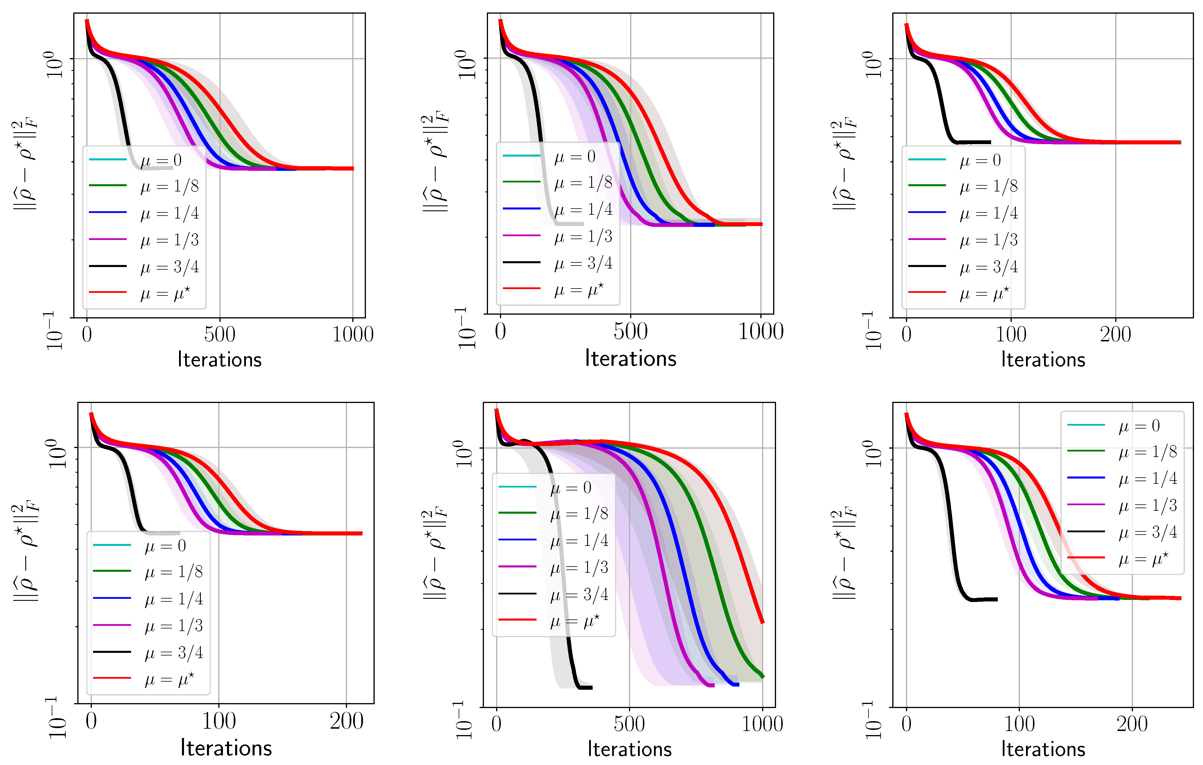
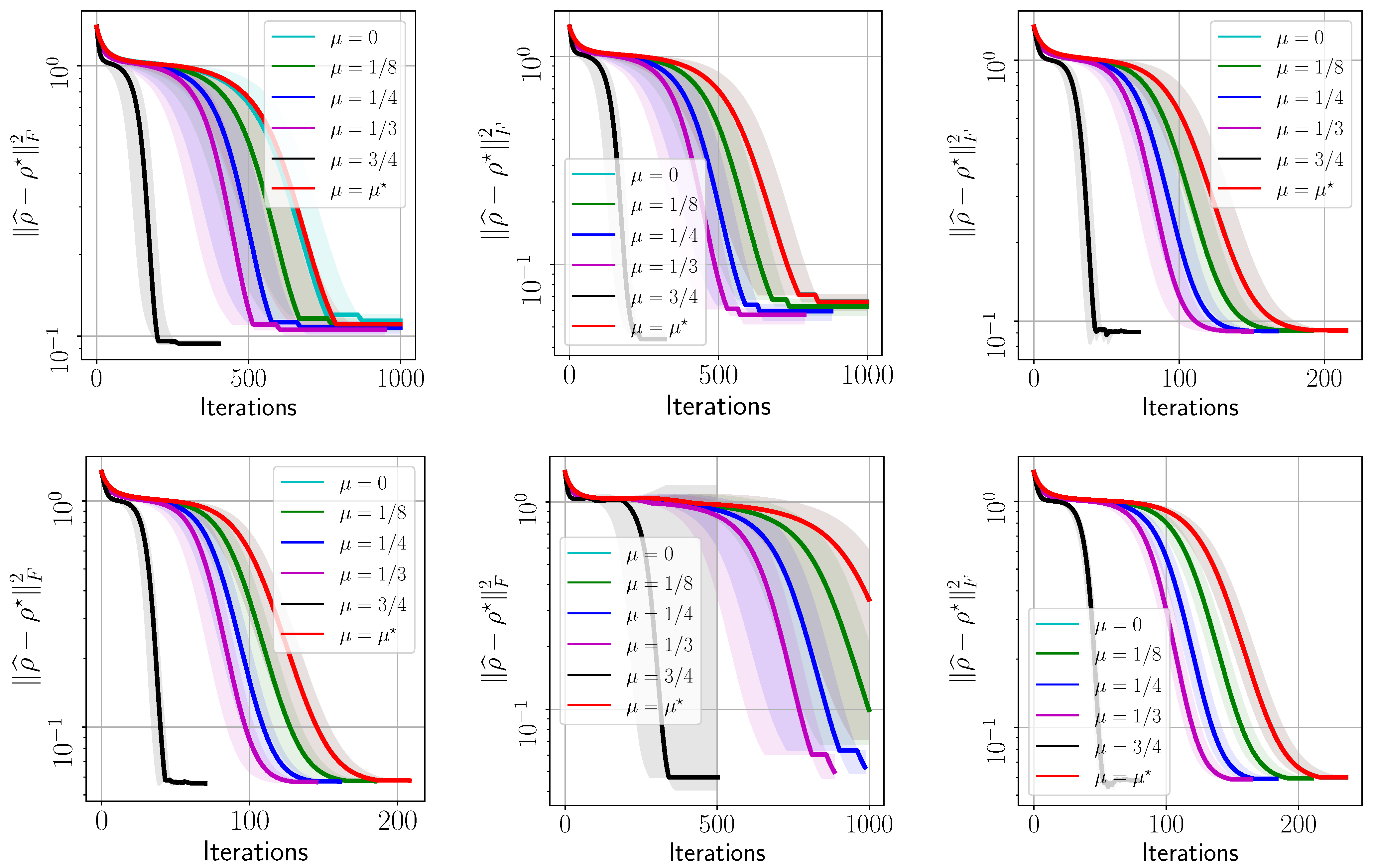
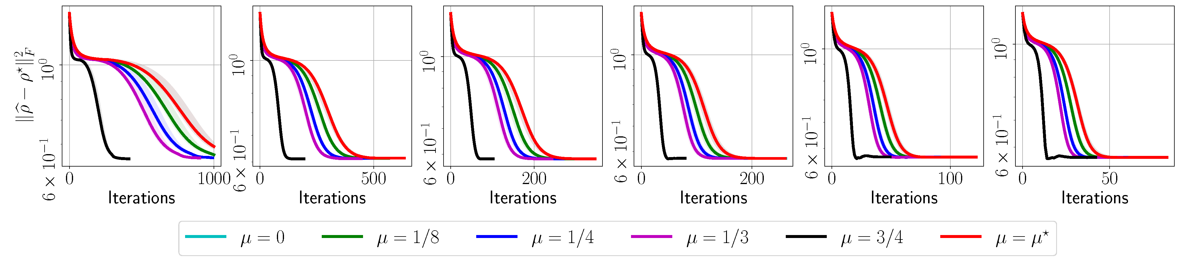
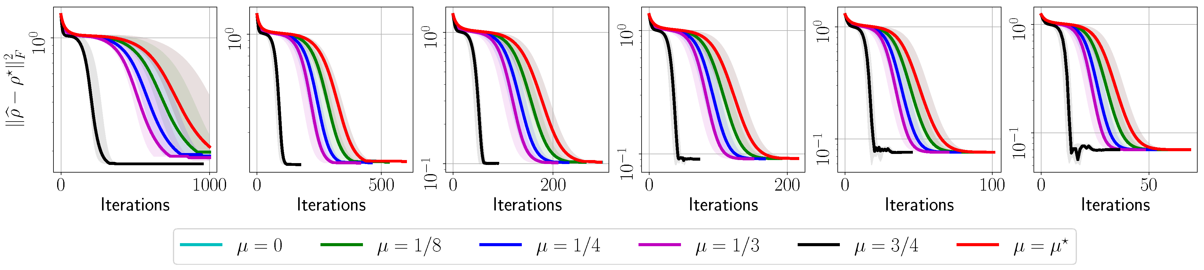
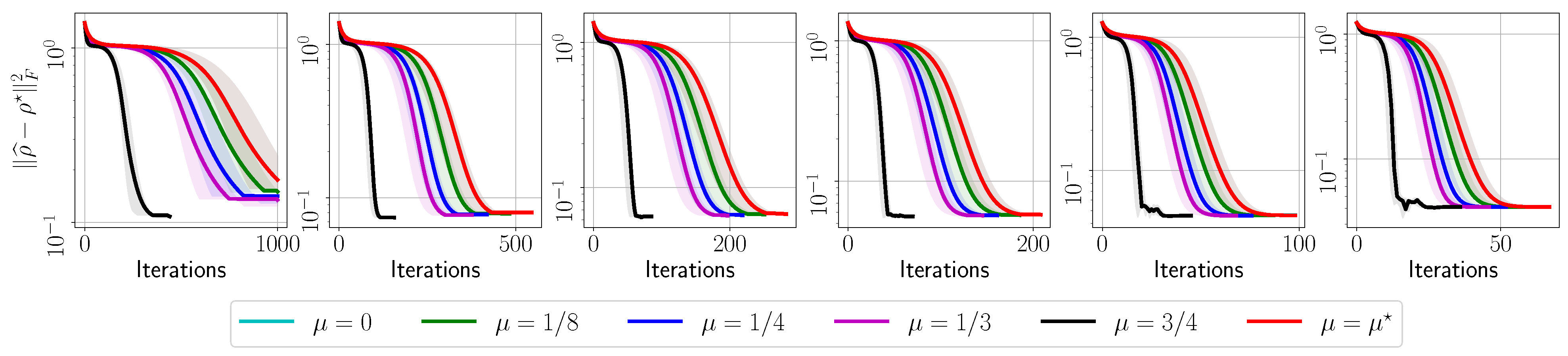
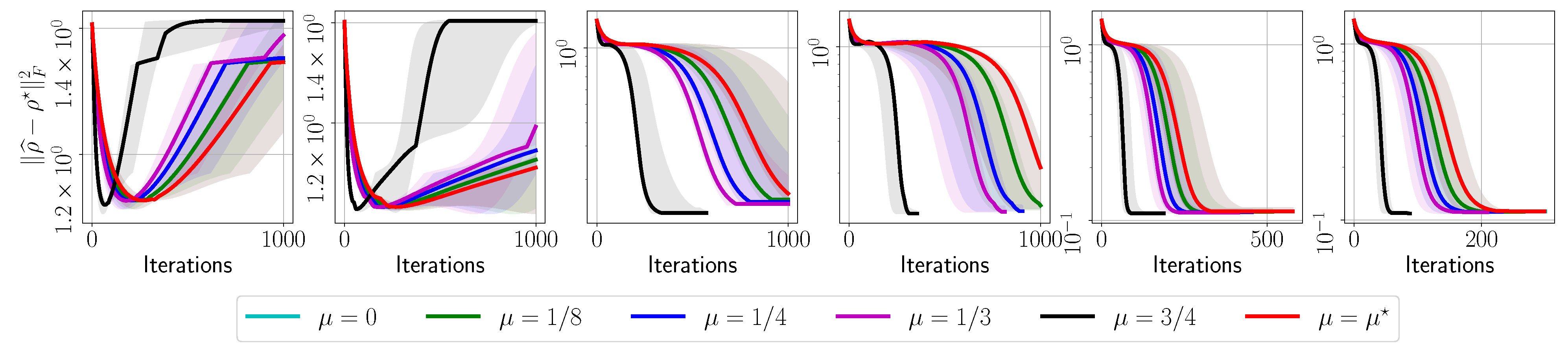
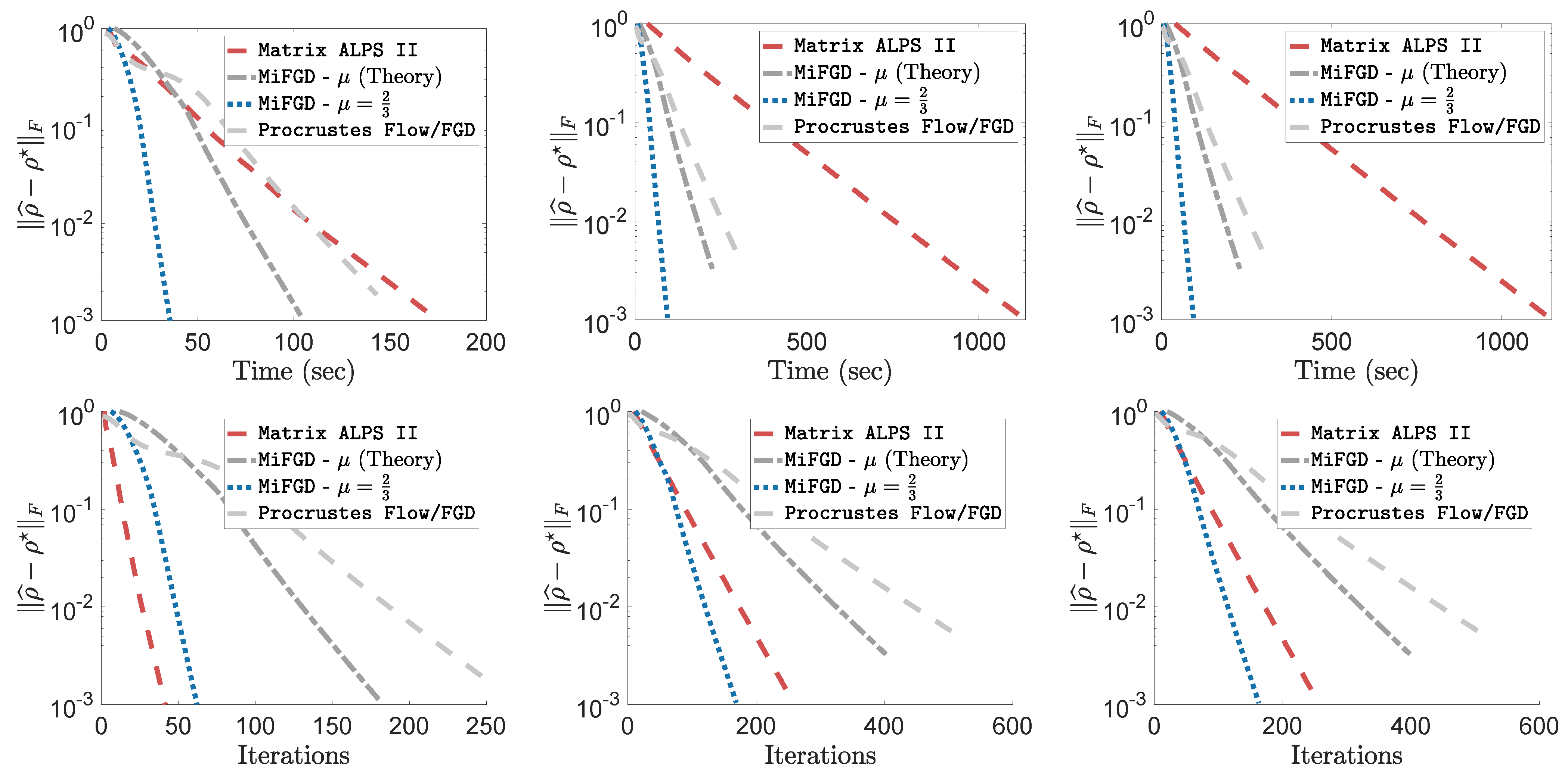
• The evolution with respect to the distance between $\widehat{\rho }$ and ${\rho }^{\star }$: $\parallel \widehat{\rho }-{\rho }^{\star }{\parallel }_F$, for various $\mu$’s.
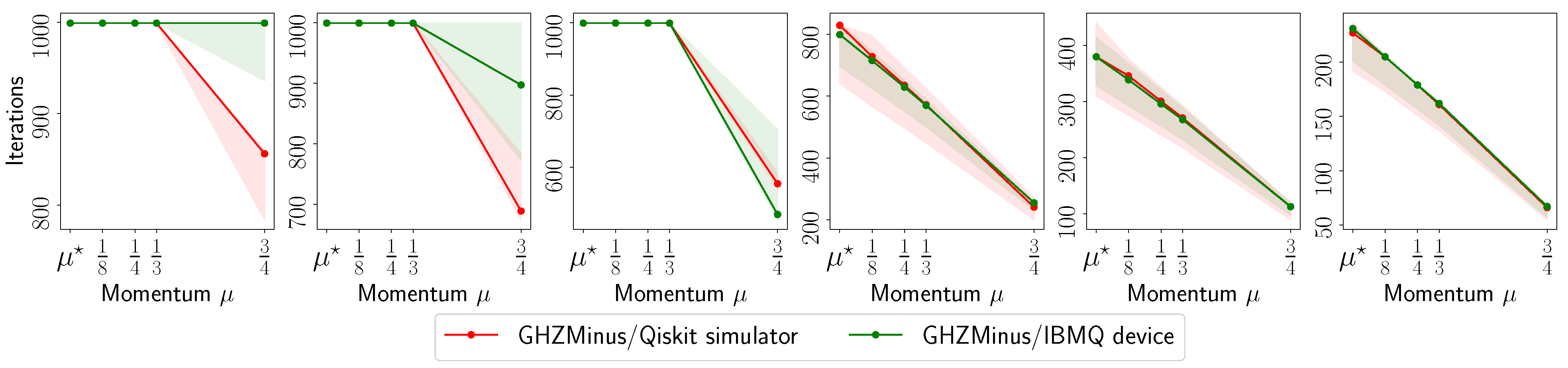
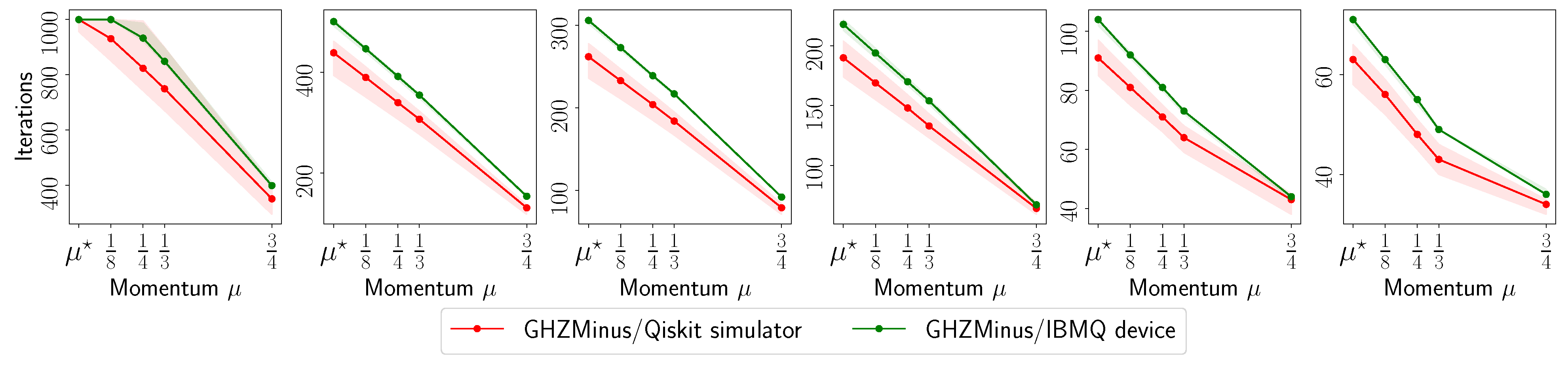
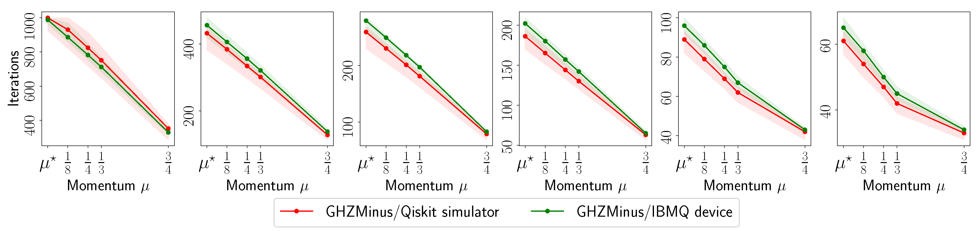
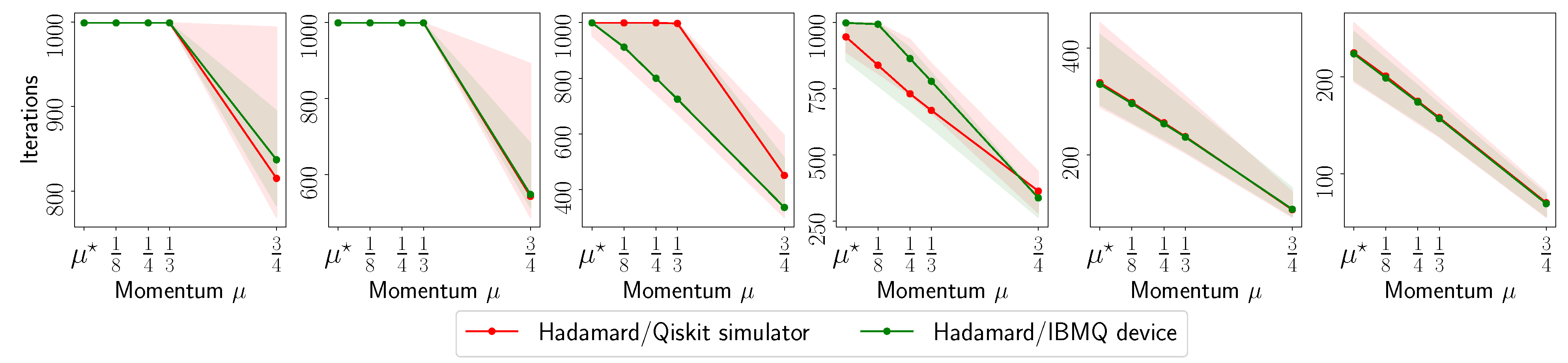
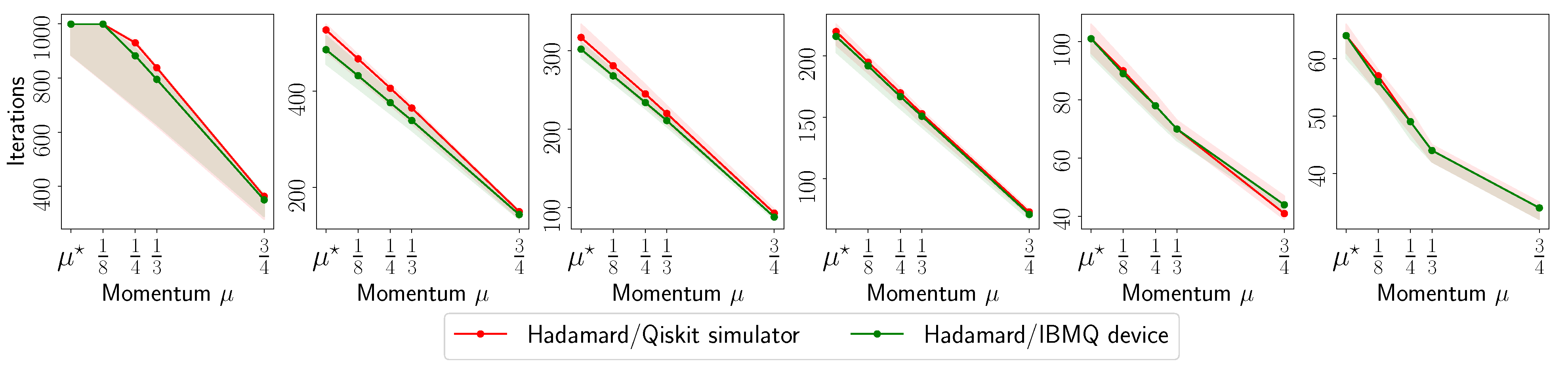
• The number of iterations to reach $\mathtt{reltol}$ to ${\rho }^{\star }$ for various $\mu$’s.
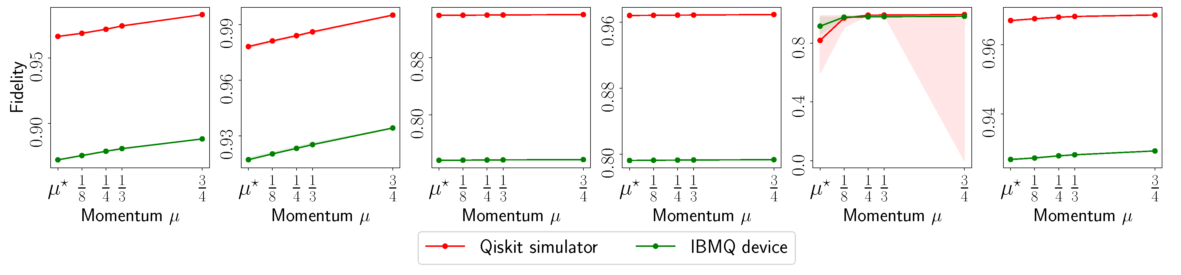
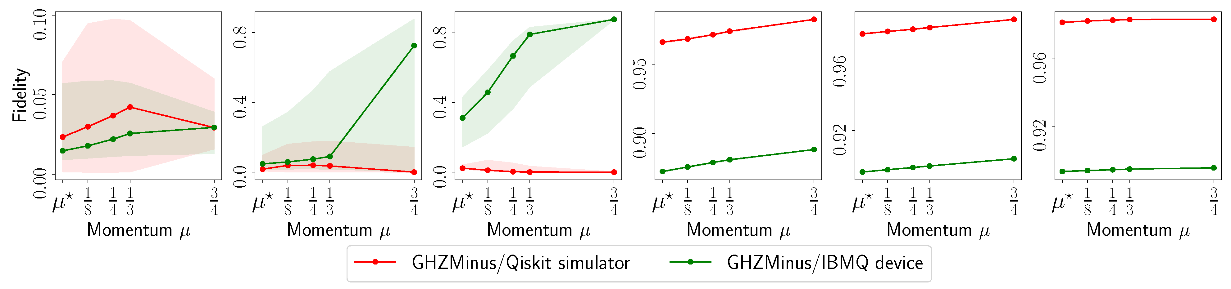
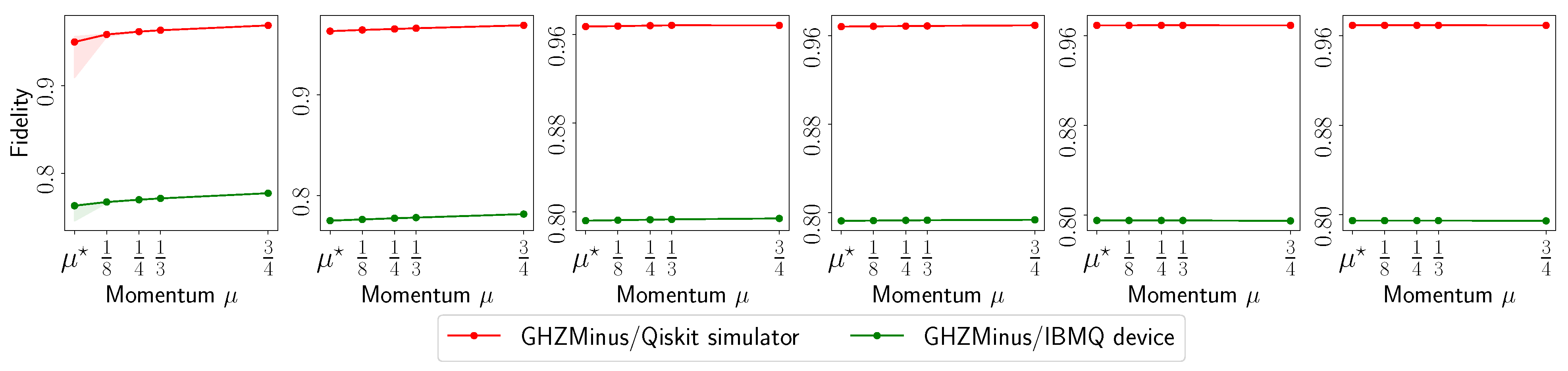
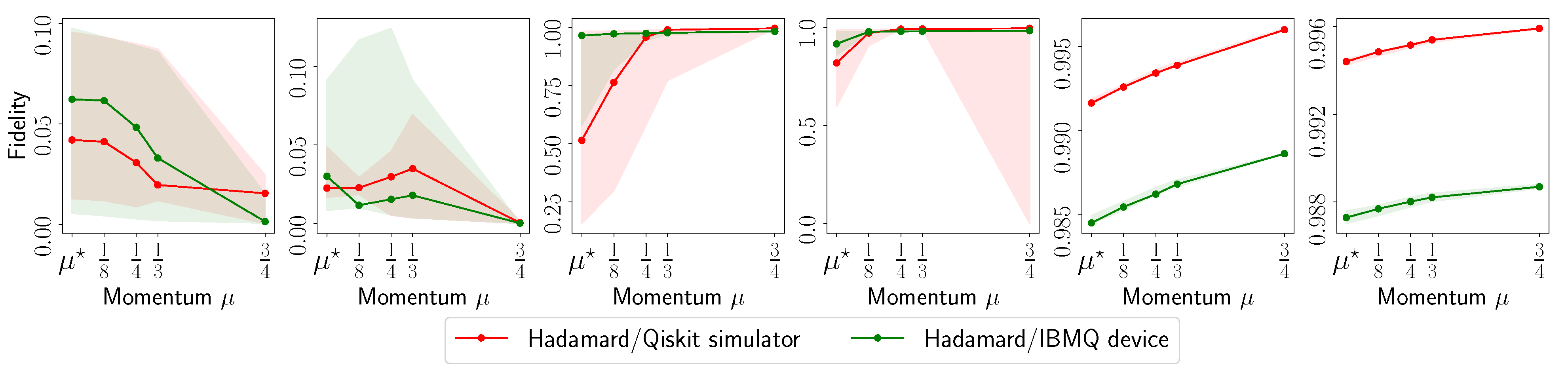
• The fidelity of $\widehat{\rho }$, defined as $\mathrm{Tr}\left({\rho }^{\star }\widehat{\rho }\right)$ (for rank-1 ${\rho }^{\star }$), as a function of the acceleration parameter $\mu$ in the default set.

In our plots, we sweep over our default set of measpc values, repeat 5 times for each individual setup, varying supplied seed, and depict their 25-, 50- and 75-percentiles.

3.4. Experimental Setup on Quantum Processing Unit (QPU)

We show empirical results on 6- and 8-qubit real data, obtained on the 20-qubit IBM QPU ibmq_boeblingen. The layout/connectivity of the device is shown in Figure 1. The 6-qubit data was from qubits $[0,1,2,3,8,9]$, and the 8-qubit data was from $[0,1,2,3,8,9,6,4]$. The $T_1$ coherence times are $[39.1,75.7,66.7,100.0,120.3,39.2,70.7,132.3]$ $\mu s$, and $T_2$ coherence times are $[86.8,94.8,106.8,63.6,156.5,66.7,104.5,134.8]$ $\mu s$. The circuit for generating 6-qubit and 8-qubit GHZ states are shown in Figure 1. The typical two qubit gate errors measured from randomized benchmarking (RB) for relevant qubits are summarized in Table 1.

The QST circuits were generated using the tomography module in qiskit-ignis (https://github.com/Qiskit/qiskit-ignis (accessed on 18 January 2023)). For complete QST of a n-qubits state $3^n$ circuits are needed. The result of each circuit is averaged over 8192, 4096 or 2048, for different n-qubit scenarios. To mitigate for readout errors, we prepare and measure all of the $2^n$ computational basis states in the computation basis to construct a calibration matrix C. C has dimension $2^n$ by $2^n$, where each column vector corresponds to the measured outcome of a prepared basis state. In the ideal case of no readout error, C is an identity matrix. We use C to correct for the measured outcomes of the experiment by minimizing the function:

$$\begin{array}{ccccccc}\hfill & {\displaystyle \underset{v^{\mathrm{cal}}\in {\mathbb{R}}^d}{\min }}\hfill & \hfill & \parallel C{v}^{\mathrm{cal}}-v^{\mathrm{meas}}{\parallel }^2\hfill & \hfill \mathrm{subject}\mathrm{to}& \hfill & \hfill {\displaystyle \sum _i}{v}_i^{\mathrm{cal}}=1,v_i^{\mathrm{cal}}\ge 0,\forall i=1,\dots ,d\end{array}$$

(12)

Here $v^{\mathrm{meas}}$ and $v^{\mathrm{cal}}$ are the measured and calibrated outputs, respectively. The minimization problem is then formulated as a convex optimization problem and solved by quadratic programming using the package cvxopt [49].

4. Results

4.1. MiFGD on 6- and 8-Qubit Real Quantum Data

We realize two types of quantum states on IBM QPUs, parameterized by the number of qubits n for each case: the ${\mathtt{GHZ}}_{-}\left(n\right)$ and the $\mathtt{Hadamard}\left(n\right)$ circuits. We collected measurements over all possible Pauli settings by repeating the experiment for each setting a number of times: these are the number of shots for each setting. The (circuit, number of shots) measurement configurations from IBM Quantum devices are summarized in Table 2.

In Appendix A, we provide target error list plots for the evolution of $\parallel \widehat{\rho }-{\rho }^{\star }{\parallel }_F^2$ for reconstructing all the settings in Table 2, both for real data and for simulated scenarios. Further, we provide plots that relate the effect of momentum acceleration on the final fidelity observed for these cases. For clarity, in Figure 2, we summarize the efficiency of momentum acceleration, by showing the reconstruction error only for the following settings: $\mathtt{maxiters}=1000$, $\eta ={10}^{-3}$, $\mathtt{reltol}=5\times {10}^{-4}$, and $\mathtt{measpc}=20\%$. In the plots, $\mu =0$ corresponds to the FGD algorithm in [30], ${\mu }^{\star }$ corresponds to the value obtained through our theory, while we use $\mu \in \left\{\frac{1}{8},\frac{1}{4},\frac{1}{3},\frac{3}{4}\right\}$ to study the acceleration effect. For ${\mu }^{\star }$, per our theory, we follow the rule ${\mu }^{\star }\approx {\epsilon }_{\mu }/2211$ for ${\epsilon }_{\mu }\in (0,1]$; see also Section 2 for details (For this application, ${\sigma }_r\left({\rho }^{\star }\right)=1$, $\tau \left({\rho }^{\star }\right)=1$, and $r=1$ by construction; we also approximated $\kappa =1.223$, which, for user-defined ${\epsilon }_{\mu }=1$, results in ${\mu }^{\star }=4.5\times {10}^{-4}$. Note that smaller ${\epsilon }_{\mu }$ values result into a smaller radius of the convergence region; however, more pessimistic ${\epsilon }_{\mu }$ values result into small $\mu$, with no practical effect in accelerating the algorithm). Note that, in most of the cases, the curve corresponding to $\mu =0$ is hidden behind the curve corresponding to $\mu \approx {\mu }^{\star }$. We run each QST experiment for 5 times for random initializations. We record the evolution of the $\parallel \widehat{\rho }-{\rho }^{\star }{\parallel }_F^2$ error at each step, and stop when the relative error of successive iterates gets smaller than $\mathtt{reltol}$ or the number of iterations exceeds $\mathtt{maxiters}$ (whichever happens first). To implement $\mathtt{measpc}=20\%$, we follow the description given in Equation (11) with $m=\mathtt{measpc}·d^2$.

To highlight the level of noise existing in real quantum data, in Figure 3, we repeat the same setting using the QASM simulator in qiskit-aer. This is a parallel, high performance quantum circuit simulator written in C++ that can support a variety of realistic circuit level noise models.

Figure 2 summarizes the performance of our proposal on different ${\rho }^{\star }$, and for different $\mu$ values on real IBM QPU data. All plots show the evolution of $\parallel \widehat{\rho }-{\rho }^{\star }{\parallel }_F$ across iterations, featuring a steep dive to convergence for the largest value of $\mu$ we tested: we report that we also tested $\mu =0$, which shows only slight worse performances than ${\mu }^{\star }$. Figure 2 highlights the universality of our approach: its performance is oblivious to the quantum state reconstructed, as long as it satisfies purity or it is close to a pure state. Our method does not require any additional structure assumptions in the quantum state.

To highlight the effect of real noise on the performance of MiFGD, we further plot its performance on the same settings but using measurements coming from an idealized quantum simulator. Figure 3 considers the exact same settings as in Figure 2. It is obvious that MiFGD can achieve better reconstruction performance when data are less erroneous. This also highlights that, in real noisy scenarios, the radius of the convergence region of MiFGD around ${\rho }^{\star }$ is controlled mostly by the the noise level, rather than by the inclusion of momentum acceleration.

Finally, in Figure 4, we depict the fidelity of $\widehat{\rho }$ achieved using MiFGD, defined as $\mathrm{Tr}\left({\rho }^{\star }\widehat{\rho }\right)$, versus various $\mu$ values and for different circuits $\left({\rho }^{\star }\right)$. Shaded area denotes standard deviation around the mean over repeated runs in all cases. The plots show the significant gap in performance when using real quantum data versus using synthetic simulated data within a controlled environment.

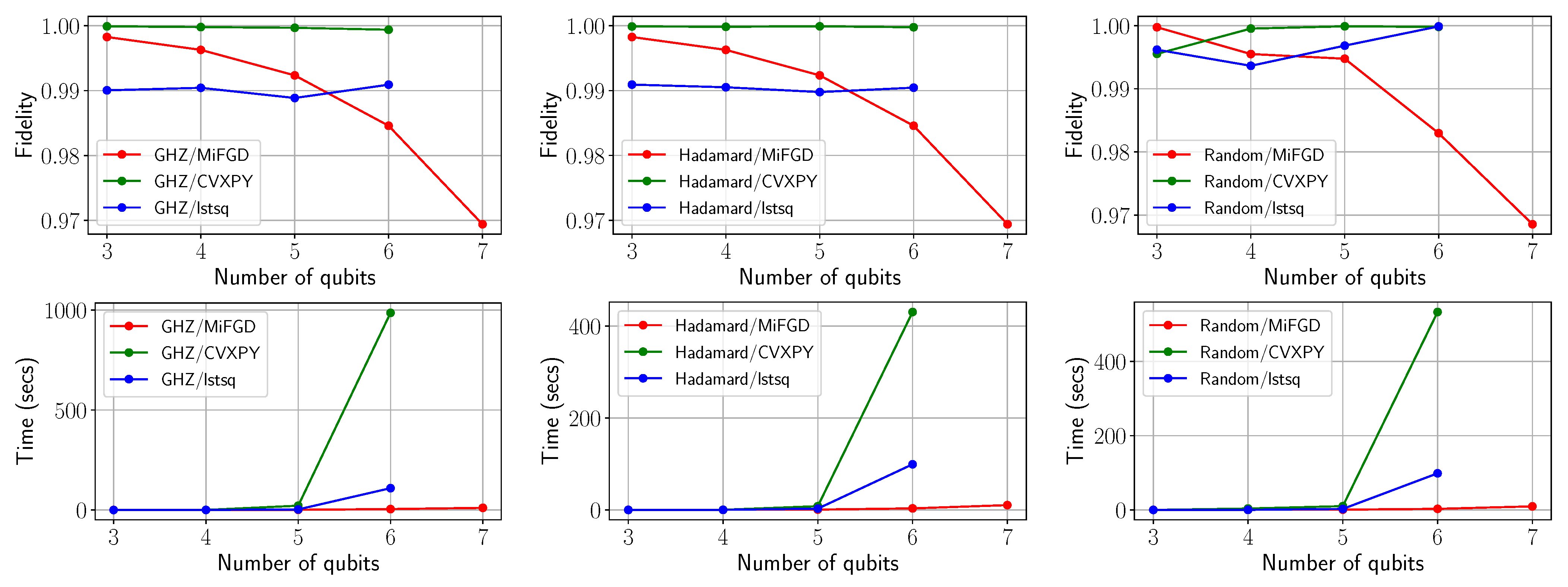
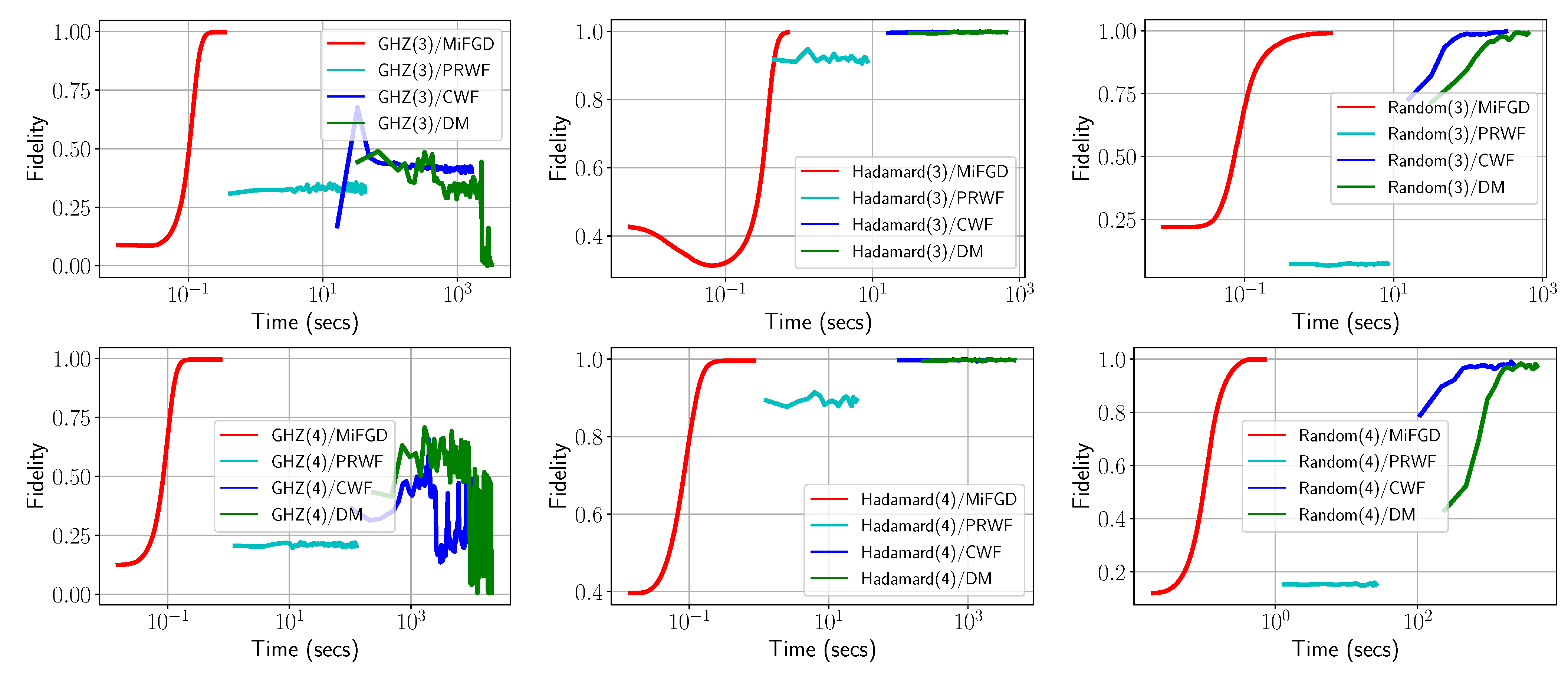
4.2. Performance Comparison with Full Tomography Methods in Qiskit

We compare the MiFGD with publicly available implementations for QST reconstruction. Two common techniques for QST, included in the qiskit-ignis distribution [28], are: (i) the CVXPY fitter method, that uses the CVXPY convex optimization package [50,51]; and (ii) the lstsq method, that uses least-squares fitting [52]. Both methods solve the full tomography problem (In [8], it was sown that the minimization program (13) yields a robust estimation of low-rank states in the compressed sensing. Thus, one can use CVXPY fitter method to solve Equation (13) with $m\ll d^2$ Pauli expectation value to obtain a robust reconstruction of ${\rho }^{\star }$) according to the following expression:

$$\begin{array}{cccc}\hfill & {\displaystyle \underset{\rho \in {\mathbb{C}}^{d\times d}}{\min }}\hfill & \hfill & f\left(\rho \right):=\frac{1}{2}{\parallel \mathcal{A}\left(\rho \right)-y\parallel }_2^2\hfill \\ \hfill & \mathrm{subject}\mathrm{to}\hfill & \hfill & \rho ⪰0,\mathtt{Tr}\left(\rho \right)=1.\hfill \end{array}$$

(13)

We note that MiFGD is not restricted to “tall” U scenarios to encode PSD and rank constraints: even without rank constraints, one could still exploit the matrix decomposition $\rho =U{U}^{†}$ to avoid the PSD projection, $\rho ⪰0$, where $U\in {\mathbb{C}}^{d\times d}$. For the lstsq fitter method, the putative estimate $\widehat{\rho }$ is rescaled using the method proposed in [52]. For CVXPY, the convex constraint makes the optimization problem a semidefinite programming (SDP) instance. By default, CVXPY calls the SCS solver that can handle all problems (including SDPs) [53,54]. Further comparison results with matrix factorization techniques from the machine learning community is provided in the Appendix for $n=12$.

The settings we consider for full tomography are the following: $\mathtt{GHZ}\left(n\right)$, $\mathtt{Hadamard}\left(n\right)$ and $\mathtt{Random}\left(n\right)$ quantum states (for $n=3,\dots ,8$). We focus on fidelity of reconstruction and computation timings performance between $\mathtt{CVXPY}$, $\mathtt{lstsq}$ and $\mathtt{MiFGD}$. We use 100% of the measurements. We experimented with states simulated in QASM and measured taking 2048 shots. For MiFGD, we set $\eta =0.001$, $\mu =\frac{3}{4}$, and stopping criterion/tolerance $\mathtt{reltol}={10}^{-5}$. All experiments are run on a Macbook Pro with 2.3 GHz Quad-Core Intel Core i7CPU and 32GB RAM.

The results are shown in Figure 5; higher-dimensional cases are provided in Table 3. Some notable remarks: (i) For small-scale scenarios ($n=3,4$), CVXPY and lstsq attain almost perfect fidelity, while being comparable or faster than MiFGD. (ii) The difference in performance becomes apparent from $n=6$ and on: while MiFGD attains 98% fidelity in <5 s, CVXPY and lstsq require up to hundreds of seconds to find a good solution. (iii) Finally, while MiFGD gets to high-fidelity solutions in seconds for $n=7,8$, CVXPY and lstsq methods could not finish tomography as their memory usage exceeded the system’s available memory.

It is noteworthy that the reported fidelities for MiFGD are the fidelities at the last iteration, before the stopping criterion is activated, or the maximum number of iterations is exceeded. However, the reported fidelity is not necessarily the best one during the whole execution: for all cases, we observe that MiFGD finds intermediate solutions with fidelity >99%. Though, it is not realistic to assume that the iteration with the best fidelity is known a priori, and this is the reason we report only the final iteration fidelity.

4.3. Performance Comparison of MiFGD with Neural-Network Quantum State Tomography

We compare the performance of MiFGD with neural network approaches. Per [9,10,11,27], we model a quantum state with a two-layer Restricted Boltzmann Machine (RBM). RBMs are stochastic neural networks, where each layer contains a number of binary stochastic variables: the size of the visible layer corresponds to the number of input qubits, while the size of the hidden layer is a hyperparameter controlling the representation error. We experiment with three types of RBMs for reconstructing either the positive-real wave function, the complex wave function, or the density matrix of the quantum state. In the first two cases the state is assumed pure while in the last, general mixed quantum states can be represented. We leverage the implementation in QuCumber [10], PositiveRealWaveFunction (PRWF), ComplexWaveFunction (CWF), and DensityMatrix (DM), respectively.

We reconstruct $\mathtt{GHZ}\left(n\right)$, $\mathtt{Hadamard}\left(n\right)$ and $\mathtt{Random}\left(n\right)$ quantum states (for $n=3,\dots ,8$), by training PRWF, CWF, and DM neural networks (We utilize GPU (NVidia GeForce GTX 1080 TI,11GB RAM) for faster training of the neural networks) with measurements collected by the QASM Simulator.

For our setting, we consider measpc = 50% and shots = 2048. The set of measurements is presented to the RBM implementation, along with the target positive-real wave function (for PRWF), complex wavefunction (for CWF) or the target density matrix (for DM) in a suitable format for training. We train Hadamard and Random states with 20 epochs, and GHZ state with 100 epochs (We experimented higher number of epochs (up to 500) for all cases, but after the reported number of epochs, Qucumber methods did not improve, if not worsened). We set the number of hidden variables (and also of additional auxilliary variables for DM) to be equal to the number of input variables n and we use 100 data points for both the positive and the negative phase of the gradient (as per the recommendation for the defaults). We choose $k=10$ contrastive divergence steps and fixed the learning rate to 10 (per hyperparameter tuning). Lastly, we limit the fitting time of Qucumber methods (excluding data preparation time) to be three hours. To compare to the RBM results, we run MiFGD with $\eta =0.001$, $\mu =\frac{3}{4}$, $\mathtt{reltol}={10}^{-5}$ and using measpc = 50%, keeping previously chosen values for all other hyperparameters.

We report the fidelity of the reconstruction as a function of elapsed training time for $n=3,4$ in Figure 6 for PRWF, CWF, and DM. We observe that for all cases, Qucumber methods are orders of magnitude slower than MiFGD. E.g., for $n=8$, for all three states, CWF and DM did not finish a single epoch in 3 h, while MiFG achieves high fidelity in less than 30 s. For the $\mathtt{Hadamard}\left(n\right)$ and $\mathtt{Random}\left(n\right)$, reaching reasonable fidelities is significantly slower for both CWF and DM, while PRWF hardly improves its performance throughout the training. For the GHZ case, CWF and DM also shows non-monotonic behaviors: even after a few thousands of seconds, fidelities have not “stabilized”, while PRWF stabilizes in very low fidelities. In comparison MiFGD is several orders of magnitude faster than both CWF and DM and fidelity smoothly increases to comparable or higher values. Further, in Table 4, we report final fidelities (within the 3 h time window), and reported times.

4.4. The Effect of Parallelization

We study the effect of parallelization in running MiFGD. We parallelize the iteration step across a number of processes, that can be either distributed and network connected, or sharing memory in a multicore environment. Our approach is based on Message Passing Interface (MPI) specification [55], which is the lingua franca for interprocess communication in high performance parallel and supercomputing applications. A MPI implementation provides facilities for launching processes organized in a virtual topology and highly tuned primitives for point-to-point and collective communication between them.

We assign to each process a subset of the measurement labels consumed by the parallel computation. At each step, a process first computes the local gradient-based corrections due only to its assigned Pauli monomials and corresponding measurements. These local gradient-based corrections will then (i) need to be communicated, so that they can be added, and (ii) finally, their sum will be shared across all processes to produce a global update for U for next step. We accomplish this structure in MPI using MPI_Allreduce collective communication primitive with MPI_SUM as its reduction operator: the underlying implementation will ensure minimum communication complexity for the operation (e.g., $\log p$ steps for p processes organized in a communication ring) and thus maximum performance (This communication pattern can alternatively be realized in two stages, as naturally suggested in its structure: (i) first invoke MPI’s MPI_Reduce primitive, with MPI_SUM as its reduction operator, which results in the element-wise accumulation of local corrections (vector sum) at a single, designated root process, and (ii) finally, send a “copy” of this sum from root process to each process participating in the parallel computation (broadcasting); MPI_Bcast primitive can be utilized for this latter stage. However, MPI_Allreduce is typically faster, since its actual implementation is not constrained by the requirement to have the sum available at a specific, root process, at an intermediate time point - as the two-stage approach implies). We leverage mpi4py [56] bindings to issue MPI calls in our parallel Python code.

We conducted our parallel experiments on a server equipped with 4 × E7-4850 v2 CPUs @ 2.30GHz (48/96 physical/virtual cores), 256 GB RAM, using shared memory multiprocessing over multiple cores. We experimented with states simulated in QASM and measured taking 8192 shots; parallel MiFGD runs with default parameters and using all measurements (measpc = 100%). Reported times are wall-clock computation time. These exclude initialization time for all processes to load Pauli monomials and measurements: we here target parallelizing computation proper in MiFGD.

In our first round of experiments, we investigate the scalability of our approach. We vary the number p of parallel processes ($p=1,2,4,8,16,32,48,64,80,96$), collect timings for reconstructing $\mathtt{GHZ}\left(4\right)$, $\mathtt{Random}\left(6\right)$ and ${\mathtt{GHZ}}_{-}\left(8\right)$ states and report speedups $T_p/T_1$ we gain from MiFGD in Figure 7 Left. We observe that the benefits of parallelization are pronounced for bigger problems (here: $n=8$ qubits) and maximum scalability results when we use all physical cores (48 in our platform).

Further, we move to larger problems ($n=10$ qubits: reporting on reconstructing $\mathtt{Hadamard}\left(10\right)$ state) and focus on the effect parallelization to achieving a given level of fidelity in reconstruction. In Figure 7 Middle, we illustrate the fidelity as a function of the time spent in the iteration loop of MiFGD for ($p=8,16,32,48,64$): we observe the smooth path to convergence in all p counts which again minimizes compute time for $p=48$. Note that in this case we use measpc = 10% and $\mu =\frac{1}{4}$.

Finally, in Figure 7 Right, we fix the number of processes to $p=48$, in order to minimize compute time and increase the percentage of used measurements to $20\%$ of the total available for $\mathtt{Hadamard}\left(10\right)$. We vary the acceleration parameter, $\mu =0$ (no acceleration) to $\mu =\frac{1}{4}$ and confirm that we indeed get faster convergence times in the latter case while the fidelity value remains the same (i.e., coinciding upper plateau value in the plots). We can also compare with the previous fidelity versus time plot, where the same $\mu$ but half the measurements are consumed: more measurements translate to faster convergence times (plateau is reached roughly $25\%$ faster; compare the green line with the yellow line in the previous plot).

5. Conclusions and Discussions

We have introduced the MiFGD algorithm for the factorized form of the low-rank QST problems. We proved that, under certain assumptions on the problem parameters, MiFGD converges linearly to a neighborhood of the optimal solution, whose size depends on the momentum parameter $\mu$, while using acceleration motions in a non-convex setting. We demonstrate empirically, using both simulated and real data, that MiFGD outperforms non-accelerated methods on both the original problem domain and the factorized space, contributing to recent efforts on testing QST algorithms in real quantum data [22]. These results expand on existing work in the literature illustrating the promise of factorized methods for certain low-rank matrix problems. Finally, we provide a publicly available implementation of our approach, compatible to the open-source software Qiskit [28], where we further exploit parallel computations in MiFGD by extending its implementation to enable efficient, parallel execution over shared and distributed memory systems.

Despite our theory does not apply to the Pauli basis measurement directly (i.e., using randomly selected Pauli bases ${\mathrm{\Pi }}_{\alpha }$, does not lead to the ${\ell }_2$-norm RIP), using the data from random Pauli basis measurements directly could provide excellent tomographic reconstruction with MiFGD. Preliminary results suggest that only $O(r·\log d)$ random Pauli bases should be taken for a reconstruction, with the same level of accuracy as with $O(r·d·\log d)$ expectation values of random Pauli matrices. We leave the analysis of our algorithm in this case for future work, along with detailed experiments.

Related Work

Matrix sensing. The problem of low-rank matrix reconstruction from few samples was first studied within the paradigm of convex optimization, using the nuclear norm minimization [29,57,58]. The use of non-convex approaches for low-rank matrix recovery—by imposing rank-constraints—has been proposed in [59,60,61]. In all these works, the convex and non-convex algorithms involve a full, or at least a truncated, singular value decomposition (SVD) per algorithm iteration. Since SVD can be prohibitive, these methods are limited to relatively small system sizes.

Momentum acceleration methods are used regularly in the convex setting, as well as in machine learning practical scenarios [62,63,64,65,66,67]. While momentum acceleration was previously studied in non-convex programming setups, it mostly involve non-convex constraints with a convex objective function [47,61,68,69]; and generic non-convex settings but only considering with the question of whether momentum acceleration leads to fast convergence to a saddle point or to a local minimum, rather than to a global optimum [45,70,71,72].

The factorized version for semi-definite programming was popularized in [73]. Effectively the factorization of a the set of PSD matrices to a product of rectangular matrices results in a non-convex setting. This approach have been heavily studied recently, due to computational and space complexity advantages [25,26,30,31,32,33,34,36,37,38,41,74,75,76]. None of the works above consider the inclusion and analysis of momentum. Moreover, the Procrustes Flow approach [32,34] uses certain initializations techniques, and thus relies on multiple SVD computations. Our approach on the other hand uses a single, unique, top-r SVD computation. Comparison results beyond QST are provided in the appendix.

Compressed sensing QST using non-convex optimization. There are only few works that study non-convex optimization in the context of compressed sensing QST. The authors of [16] propose a hybrid algorithm that (i) starts with a conjugate-gradient (CG) algorithm in the factored space, in order to get initial rapid descent, and (ii) switch over to accelerated first-order methods in the original $\rho$ space, provided one can determine the switch-over point cheaply. Using the multinomial maximum likelihood objective, in the initial CG phase, the Hessian of the objective is computed per iteration (i.e., a $4^n\times 4^n$ matrix), along with its eigenvalue decomposition. Such an operation is costly, even for moderate values of qubit number n, and heuristics are proposed for its completion. From a theoretical perspective, [16] provide no convergence or convergence rate guarantees.

From a different perspective, [77] relies on spectrum estimation techniques [78,79] and the Empirical Young Diagram algorithm [80,81] to prove that $O(rd/\epsilon )$ copies suffice to obtain an estimate $\widehat{\rho }$ that satisfies $\parallel \widehat{\rho }-{\rho }^{\star }{\parallel }_F^2\le \epsilon$; however, to the best of our knowledge, there is no concrete implementation of this technique to compare with respect to scalability.

Ref. [82] proposes an efficient quantum tomography protocol by determining the permutationally invariant part of the quantum state. The authors determine the minimal number of local measurement settings, which scales quadratically with the number of qubits. The paper determines which quantities have to be measured in order to get the smallest uncertainty possible. See [83] for a more recent work on permutationally invariant tomography. The method has been tested in a six-qubit experiment in [84].

Ref. [22] presented an experimental implementation of compressed sensing QST of a $n=7$ qubit system, where only 127 Pauli basis measurements are available. To achieve recovery in practice, the authors proposed a computationally efficient estimator, based on gradient descent method in the factorized space. The authors of [22] focus on the experimental efficiency of the method, and provide no specific results on the optimization efficiency, neither convergence guarantees of the algorithm. Further, there is no available implementation publicly available.

Similar to [22], Ref. [26] also proposes a non-convex projected gradient decent algorithm that works on the factorized space in the QST setting. The authors prove a rigorous convergence analysis and show that, under proper initialization and step-size, the algorithm is guaranteed to converge to the global minimum of the problem, thus ensuring a provable tomography procedure. Our results extend these results by including acceleration techniques in the factorized space. The key contribution of our work is proving convergence of the proposed algorithm in a linear rate to the global minimum of the problem, under common assumptions. Proving our results required developing a whole set of new techniques, which are not based on a mere extension of existing results.

Compressed sensing QST using convex optimization. The original formulation of compressed sensing QST [4] is based on convex optimization methods, solving the trace-norm minimization, to obtain an estimation of the low-rank state. It was later shown [8] that essentially any convex optimization program can be used to robustly estimate the state. In general, there are two drawbacks in using convex optimization optimization in QST. Firstly, as the dimension of density matrices grow exponentially in the number of qubits, the search space in convex optimization grows exponentially in the number of qubits. Secondly, the optimization requires projection onto the PSD cone at every iteration, which becomes exponentially hard in the number of qubits. We avoid these two drawbacks by working in the factorized space. Using this factorization results in a search space that is substantially smaller than its convex counterpart, and moreover, in a single use of top-r SVD during the entire execution algorithm. Bypassing these drawbacks, together with accelerating motions, allows us to estimate quantum states of larger qubit systems than state-of-the-art algorithms.

Full QST using non-convex optimization. The use of non-convex algorithms in QST was studied in the context of full tomography as well. By “full tomography” we refer to the situation where an informationally complete measurement is performed, so that the input data to the algorithm is of size $4^n$. The exponential scaling of the data size restrict the applicability of full tomography to relatively small system sizes. In this setting non-convex algorithms which work in the factored space were studied [85,86,87,88,89]. Except of the work [88], we are not aware of theoretical results on the convergence of the proposed algorithm due to the presence of spurious local minima. The authors of [88] characterize the local vs. the global behavior of the objective function under the factorization $\rho =U{U}^{†}$ and discuss how existing methods fail due to improper stopping criteria or due to the lack of algorithmic convergence results. Their work highlights the lack of rigorous convergence results of non-convex algorithms used in full quantum state tomography. There is no available implementation publicly available for these methods as well.

Full QST using convex optimization. Despite the non-scalability of full QST, and the limitation of convex optimization, a lot of research was devoted to this topic. Here, we mention only a few notable results that extend the applicability of full QST using specific techniques in convex optimization. Ref [52] shows that for given measurement schemes the solution for the maximum likelihood is given by a linear inversion scheme, followed by a projection onto the set of density matrices. More recently, the authors of [18] used a combination of the techniques of [52] with the sparsity of the Pauli matrices and the use of GPUs to perform a full QST of 14 qubits. While pushing the limit of full QST using convex optimization, obtaining full tomographic experimental data for more than a dozen qubits is significantly time-intensive. Moreover, this approach is highly centralized, in comparison to our approach that can be distributed. Using the sparsity pattern property of the Pauli matrices and GPUs is an excellent candidate approach to further enhance the performance of non-convex compressed sensing QST.

QST using neural networks. Deep neural networks are ubiquitous, with many applications to science and industry. Recently, [9,10,11,27] show how machine learning and neural networks can be used to perform QST, driven by experimental data. The neural network architecture used is based on restricted Boltzmann machines (RBMs) [90], which feature a visible and a hidden layer of stochastic binary neurons, fully connected with weighted edges. Test cases considered include reconstruction of W state, magnetic observables of local Hamiltonians, the unitary dynamics induced by Hamiltonian evolution. Comparison results are provided in the Main Results section. Alternative approaches include conditional generative adversarial networks (CGANs) [91,92]: in this case, two dueling neural networks, a generator and a discriminator, learn to generate and identify multi-modal models from data.

QST for Matrix Product States (MPS). This is the case of highly structured quantum states where the state is well-approximated by a MPS of low bond dimension [12,13]. The idea behind this approach is, in order to overcome exponential bottlenecks in the general QST case, we require highly structured subsets of states, similar to the assumptions made in compressed sensing QST. MPS QST is considered an alternative approach to reduce the computational and storage complexity of QST.

Direct fidelity estimation. Rather than focusing on entrywise estimation of density matrices, the direct fidelity estimation procedure focuses on checking how close is the state of the system to a target state, where closeness is quantified by the fidelity metric. Classic techniques require up to $2^n/{ϵ}^4$ number of samples, where $ϵ$ denotes the accuracy of the fidelity term, when considering a general quantum state [93,94], but can be reduced to almost dimensionality-free $1/{ϵ}^2$ number of samples for specific cases, such as stabilizer states [95,96,97]. Shadow tomography is considered as an alternative and generalization of this technique [98,99]; however, as noted in [94], the procedure in [98,99] requires exponentially long quantum circuits that act collectively on all the copies of the unknown state stored in a quantum memory, and thus has not been implemented fully on real quantum machines. A recent neural network-based implementation of such indirect QST learning methods is provided here [100].

The work in [93,94], goes beyond simple fidelity estimation, and utilizes random single qubit rotations to learn a minimal sketch of the unknown quantum state by which one that can predict arbitrary linear function of the state. Such methods constitute a favorable alternative to QST as they do not require number of samples that scale polynomially with the dimension; however, this, in turn, implies that these methods cannot be used in general to estimate the density matrix itself.

References

- Altepeter, J.B.; James, D.F.; Kwiat, P.G. 4 qubit quantum state tomography. In Quantum State Estimation; Springer: Berlin/Heidelberg, Germany, 2004; pp. 113–145. [Google Scholar]
- Eisert, J.; Hangleiter, D.; Walk, N.; Roth, I.; Markham, D.; Parekh, R.; Chabaud, U.; Kashefi, E. Quantum certification and benchmarking. arXiv 2019, arXiv:1910.06343. [Google Scholar] [CrossRef]
- Mohseni, M.; Rezakhani, A.; Lidar, D. Quantum-process tomography: Resource analysis of different strategies. Phys. Rev. A 2008, 77, 032322. [Google Scholar] [CrossRef]
- Gross, D.; Liu, Y.K.; Flammia, S.; Becker, S.; Eisert, J. Quantum state tomography via compressed sensing. Phys. Rev. Lett. 2010, 105, 150401. [Google Scholar] [CrossRef] [PubMed]
- Vogel, K.; Risken, H. Determination of quasiprobability distributions in terms of probability distributions for the rotated quadrature phase. Phys. Rev. A 1989, 40, 2847. [Google Scholar] [CrossRef]
- Ježek, M.; Fiurášek, J.; Hradil, Z. Quantum inference of states and processes. Phys. Rev. A 2003, 68, 012305. [Google Scholar] [CrossRef]
- Banaszek, K.; Cramer, M.; Gross, D. Focus on quantum tomography. New J. Phys. 2013, 15, 125020. [Google Scholar] [CrossRef]
- Kalev, A.; Kosut, R.; Deutsch, I. Quantum tomography protocols with positivity are compressed sensing protocols. NPJ Quantum Inf. 2015, 1, 15018. [Google Scholar] [CrossRef]
- Torlai, G.; Mazzola, G.; Carrasquilla, J.; Troyer, M.; Melko, R.; Carleo, G. Neural-network quantum state tomography. Nat. Phys. 2018, 14, 447–450. [Google Scholar] [CrossRef]
- Beach, M.J.; De Vlugt, I.; Golubeva, A.; Huembeli, P.; Kulchytskyy, B.; Luo, X.; Melko, R.G.; Merali, E.; Torlai, G. QuCumber: Wavefunction reconstruction with neural networks. SciPost Phys. 2019, 7, 009. [Google Scholar] [CrossRef]
- Torlai, G.; Melko, R. Machine-Learning Quantum States in the NISQ Era. Annu. Rev. Condens. Matter Phys. 2020, 11, 325–344. [Google Scholar] [CrossRef]
- Cramer, M.; Plenio, M.B.; Flammia, S.T.; Somma, R.; Gross, D.; Bartlett, S.D.; Landon-Cardinal, O.; Poulin, D.; Liu, Y.K. Efficient quantum state tomography. Nat. Comm. 2010, 1, 149. [Google Scholar] [CrossRef] [PubMed]
- Lanyon, B.; Maier, C.; Holzäpfel, M.; Baumgratz, T.; Hempel, C.; Jurcevic, P.; Dhand, I.; Buyskikh, A.; Daley, A.; Cramer, M.; et al. Efficient tomography of a quantum many-body system. Nat. Phys. 2017, 13, 1158–1162. [Google Scholar] [CrossRef]
- Gonçalves, D.; Gomes-Ruggiero, M.; Lavor, C. A projected gradient method for optimization over density matrices. Optim. Methods Softw. 2016, 31, 328–341. [Google Scholar] [CrossRef]
- Bolduc, E.; Knee, G.; Gauger, E.; Leach, J. Projected gradient descent algorithms for quantum state tomography. NPJ Quantum Inf. 2017, 3, 44. [Google Scholar] [CrossRef]
- Shang, J.; Zhang, Z.; Ng, H.K. Superfast maximum-likelihood reconstruction for quantum tomography. Phys. Rev. A 2017, 95, 062336. [Google Scholar] [CrossRef]
- Hu, Z.; Li, K.; Cong, S.; Tang, Y. Reconstructing Pure 14-Qubit Quantum States in Three Hours Using Compressive Sensing. IFAC-PapersOnLine 2019, 52, 188–193. [Google Scholar] [CrossRef]
- Hou, Z.; Zhong, H.S.; Tian, Y.; Dong, D.; Qi, B.; Li, L.; Wang, Y.; Nori, F.; Xiang, G.Y.; Li, C.F.; et al. Full reconstruction of a 14-qubit state within four hours. New J. Phys. 2016, 18, 083036. [Google Scholar] [CrossRef]
- Candes, E.; Tao, T. Near-optimal signal recovery from random projections: Universal encoding strategies? IEEE Trans. Inf. Theory 2006, 52, 5406–5425. [Google Scholar] [CrossRef]
- Gross, D. Recovering low-rank matrices from few coefficients in any basis. IEEE Trans. Inf. Theory 2011, 57, 1548–1566. [Google Scholar] [CrossRef]
- Liu, Y.K. Universal low-rank matrix recovery from Pauli measurements. In Proceedings of the Advances in Neural Information Processing Systems, Granada, Spain, 12–15 December 2011; pp. 1638–1646. [Google Scholar]
- Riofrío, C.; Gross, D.; Flammia, S.; Monz, T.; Nigg, D.; Blatt, R.; Eisert, J. Experimental quantum compressed sensing for a seven-qubit system. Nat. Commun. 2017, 8, 15305. [Google Scholar] [CrossRef]
- Kliesch, M.; Kueng, R.; Eisert, J.; Gross, D. Guaranteed recovery of quantum processes from few measurements. Quantum 2019, 3, 171. [Google Scholar] [CrossRef]
- Flammia, S.T.; Gross, D.; Liu, Y.K.; Eisert, J. Quantum tomography via compressed sensing: Error bounds, sample complexity and efficient estimators. New J. Phys. 2012, 14, 095022. [Google Scholar] [CrossRef]
- Bhojanapalli, S.; Kyrillidis, A.; Sanghavi, S. Dropping convexity for faster semi-definite optimization. In Proceedings of the Conference on Learning Theory, New York, NY, USA, 23–26 June 2016; pp. 530–582. [Google Scholar]
- Kyrillidis, A.; Kalev, A.; Park, D.; Bhojanapalli, S.; Caramanis, C.; Sanghavi, S. Provable compressed sensing quantum state tomography via non-convex methods. NPJ Quantum Inf. 2018, 4, 36. [Google Scholar] [CrossRef]
- Gao, X.; Duan, L.M. Efficient representation of quantum many-body states with deep neural networks. Nat. Commun. 2017, 8, 1–6. [Google Scholar] [CrossRef]
- tA v, A.; Anis, M.S.; Mitchell, A.; Abraham, H.; AduOffei; Agarwal, R.; Agliardi, G.; Aharoni, M.; Ajith, V.; Akhalwaya, I.Y.; et al. Qiskit: An Open-Source Framework for Quantum Computing. 2021. Available online: https://zenodo.org/record/7591922#.Y9zUYK1BxPY (accessed on 18 January 2023).
- Recht, B.; Fazel, M.; Parrilo, P.A. Guaranteed minimum-rank solutions of linear matrix equations via nuclear norm minimization. SIAM Rev. 2010, 52, 471–501. [Google Scholar] [CrossRef]
- Park, D.; Kyrillidis, A.; Caramanis, C.; Sanghavi, S. Finding low-rank solutions to matrix problems, efficiently and provably. arXiv 2016, arXiv:1606.03168. [Google Scholar]
- Park, D.; Kyrillidis, A.; Bhojanapalli, S.; Caramanis, C.; Sanghavi, S. Provable Burer-Monteiro factorization for a class of norm-constrained matrix problems. arXiv 2016, arXiv:1606.01316. [Google Scholar]
- Tu, S.; Boczar, R.; Simchowitz, M.; Soltanolkotabi, M.; Recht, B. Low-rank solutions of linear matrix equations via Procrustes flow. In Proceedings of the 33rd International Conference on International Conference on Machine Learning-Volume 48, New York, NY, USA, 19–24 June 2016; pp. 964–973. [Google Scholar]
- Zhao, T.; Wang, Z.; Liu, H. A nonconvex optimization framework for low rank matrix estimation. In Proceedings of the Advances in Neural Information Processing Systems, Montreal, QC, Canada, 7–12 December 2015; pp. 559–567. [Google Scholar]
- Zheng, Q.; Lafferty, J. A convergent gradient descent algorithm for rank minimization and semidefinite programming from random linear measurements. In Proceedings of the Advances in Neural Information Processing Systems, Montreal, QC, Canada, 7–12 December 2015; pp. 109–117. [Google Scholar]
- Cauchy, A. Méthode générale pour la résolution des systemes d’équations simultanées. Comp. Rend. Sci. Paris 1847, 25, 536–538. [Google Scholar]
- Park, D.; Kyrillidis, A.; Caramanis, C.; Sanghavi, S. Non-square matrix sensing without spurious local minima via the Burer-Monteiro approach. In Proceedings of the International Conference on Artificial Intelligence and Statistics, Ft. Lauderdale, FL, USA, 20–22 April 2017; pp. 65–74. [Google Scholar]
- Ge, R.; Jin, C.; Zheng, Y. No spurious local minima in nonconvex low rank problems: A unified geometric analysis. arXiv 2017, arXiv:1704.00708. [Google Scholar]
- Hsieh, Y.P.; Kao, Y.C.; Karimi Mahabadi, R.; Alp, Y.; Kyrillidis, A.; Cevher, V. A Non-Euclidean Gradient Descent Framework for Non-Convex Matrix Factorization. IEEE Trans. Signal Process. 2018, 66, 5917–5926. [Google Scholar] [CrossRef]
- Polyak, B. Some methods of speeding up the convergence of iteration methods. USSR Comput. Math. Math. Phys. 1964, 4, 1–17. [Google Scholar] [CrossRef]
- Nesterov, Y. A method of solving a convex programming problem with convergence rate O(1k2). Sov. Math. Dokl. 1983, 27, 372–376. [Google Scholar]
- Bhojanapalli, S.; Neyshabur, B.; Srebro, N. Global optimality of local search for low rank matrix recovery. In Proceedings of the Advances in Neural Information Processing Systems, Barcelona, Spain, 5–10 December 2016; pp. 3873–3881. [Google Scholar]
- Stöger, D.; Soltanolkotabi, M. Small random initialization is akin to spectral learning: Optimization and generalization guarantees for overparameterized low-rank matrix reconstruction. Adv. Neural Inf. Process. Syst. 2021, 34, 23831–23843. [Google Scholar]
- Lanczos, C. An Iteration Method for the Solution of the Eigenvalue Problem of Linear Differential and Integral Operators1. J. Res. Natl. Bur. Stand. 1950, 45. [Google Scholar] [CrossRef]
- Nesterov, Y. Introductory Lectures on Convex Optimization: A Basic Course; Springer Science & Business Media: Berlin, Germany, 2013; Volume 87. [Google Scholar]
- Carmon, Y.; Duchi, J.; Hinder, O.; Sidford, A. Accelerated methods for non-convex optimization. arXiv 2016, arXiv:1611.00756. [Google Scholar]
- Li, Y.; Ma, C.; Chen, Y.; Chi, Y. Nonconvex Matrix Factorization from Rank-One Measurements. In Proceedings of the International Conference on Artificial Intelligence and Statistics, Naha, Japan, 16–18 April 2019. [Google Scholar]
- Khanna, R.; Kyrillidis, A. IHT dies hard: Provable accelerated Iterative Hard Thresholding. In Proceedings of the International Conference on Artificial Intelligence and Statistics, Playa Blanca, Lanzarote, Canary Islands, 9–11 April 2018; pp. 188–198. [Google Scholar]
- Rudelson, M.; Vershynin, R. On sparse reconstruction from Fourier and Gaussian measurements. Commun. Pure Appl. Math. A J. Issued Courant Inst. Math. Sci. 2008, 61, 1025–1045. [Google Scholar] [CrossRef]
- Vandenberghe, L. The CVXOPT Linear and Quadratic Cone Program Solvers. 2010. Available online: https://www.seas.ucla.edu/vandenbe/publications/coneprog.pdf (accessed on 18 January 2023).
- Diamond, S.; Boyd, S. CVXPY: A Python-embedded modeling language for convex optimization. J. Mach. Learn. Res. 2016, 17, 1–5. [Google Scholar]
- Agrawal, A.; Verschueren, R.; Diamond, S.; Boyd, S. A rewriting system for convex optimization problems. J. Control. Decis. 2018, 5, 42–60. [Google Scholar] [CrossRef]
- Smolin, J.A.; Gambetta, J.M.; Smith, G. Efficient method for computing the maximum-likelihood quantum state from measurements with additive gaussian noise. Phys. Rev. Lett. 2012, 108, 070502. [Google Scholar] [CrossRef]
- O’Donoghue, B.; Chu, E.; Parikh, N.; Boyd, S. Conic Optimization via Operator Splitting and Homogeneous Self-Dual Embedding. J. Optim. Theory Appl. 2016, 169, 1042–1068. [Google Scholar] [CrossRef]
- O’Donoghue, B.; Chu, E.; Parikh, N.; Boyd, S. SCS: Splitting Conic Solver, Version 2.1.2. 2019. Available online: https://github.com/cvxgrp/scs (accessed on 18 January 2023).
- Forum, T.M. MPI: A Message Passing Interface. In Proceedings of the 1993 ACM/IEEE Conference on Supercomputing, Portland, OR, USA, 19 November 1993; Association for Computing Machinery: New York, NY, USA, 1993; pp. 878–883. [Google Scholar] [CrossRef]
- Dalcin, L.D.; Paz, R.R.; Kler, P.A.; Cosimo, A. Parallel distributed computing using Python. Adv. Water Resour. 2011, 34, 1124–1139. [Google Scholar] [CrossRef]
- Lee, K.; Bresler, Y. Guaranteed minimum rank approximation from linear observations by nuclear norm minimization with an ellipsoidal constraint. arXiv 2009, arXiv:0903.4742. [Google Scholar]
- Liu, Z.; Vandenberghe, L. Interior-point method for nuclear norm approximation with application to system identification. SIAM J. Matrix Anal. Appl. 2009, 31, 1235–1256. [Google Scholar] [CrossRef]
- Jain, P.; Meka, R.; Dhillon, I.S. Guaranteed rank minimization via singular value projection. In Proceedings of the Advances in Neural Information Processing Systems, Vancouver, BC, Canada, 6–9 December 2010; pp. 937–945. [Google Scholar]
- Lee, K.; Bresler, Y. Admira: Atomic decomposition for minimum rank approximation. IEEE Trans. Inf. Theory 2010, 56, 4402–4416. [Google Scholar] [CrossRef]
- Kyrillidis, A.; Cevher, V. Matrix recipes for hard thresholding methods. J. Math. Imaging Vis. 2014, 48, 235–265. [Google Scholar] [CrossRef]
- Kingma, D.; Ba, J. Adam: A method for stochastic optimization. arXiv 2014, arXiv:1412.6980. [Google Scholar]
- Tieleman, T.; Hinton, G. Lecture 6.5-RMSPro: Divide the gradient by a running average of its recent magnitude. COURSERA Neural Netw. Mach. Learn. 2012, 4, 26–31. [Google Scholar]
- Beck, A.; Teboulle, M. A fast iterative shrinkage-thresholding algorithm for linear inverse problems. SIAM J. Imaging Sci. 2009, 2, 183–202. [Google Scholar] [CrossRef]
- O’Donoghue, B.; Candes, E. Adaptive restart for accelerated gradient schemes. Found. Comput. Math. 2015, 15, 715–732. [Google Scholar] [CrossRef]
- Bubeck, S.; Lee, Y.T.; Singh, M. A geometric alternative to Nesterov’s accelerated gradient descent. arXiv 2015, arXiv:1506.08187. [Google Scholar]
- Goh, G. Why Momentum Really Works. Distill 2017, 2, e6. [Google Scholar] [CrossRef]
- Kyrillidis, A.; Cevher, V. Recipes on hard thresholding methods. In Proceedings of the Computational Advances in Multi-Sensor Adaptive Processing (CAMSAP), San Juan, PR, USA, 13–16 December 2011; pp. 353–356. [Google Scholar]
- Xu, P.; He, B.; De Sa, C.; Mitliagkas, I.; Re, C. Accelerated stochastic power iteration. In Proceedings of the International Conference on Artificial Intelligence and Statistics, Playa Blanca, Lanzarote, Canary Islands, 9–11 April 2018; pp. 58–67. [Google Scholar]
- Ghadimi, S.; Lan, G. Stochastic first-and zeroth-order methods for nonconvex stochastic programming. SIAM J. Optim. 2013, 23, 2341–2368. [Google Scholar] [CrossRef]
- Lee, J.; Simchowitz, M.; Jordan, M.; Recht, B. Gradient descent only converges to minimizers. In Proceedings of the Conference on Learning Theory, New York, NY, USA, 23–26 June 2016; pp. 1246–1257. [Google Scholar]
- Agarwal, N.; Allen-Zhu, Z.; Bullins, B.; Hazan, E.; Ma, T. Finding approximate local minima for nonconvex optimization in linear time. arXiv 2016, arXiv:1611.01146. [Google Scholar]
- Burer, S.; Monteiro, R.D. A nonlinear programming algorithm for solving semidefinite programs via low-rank factorization. Math. Program. 2003, 95, 329–357. [Google Scholar] [CrossRef]
- Jain, P.; Dhillon, I.S. Provable inductive matrix completion. arXiv 2013, arXiv:1306.0626. [Google Scholar]
- Chen, Y.; Wainwright, M.J. Fast low-rank estimation by projected gradient descent: General statistical and algorithmic guarantees. arXiv 2015, arXiv:1509.03025. [Google Scholar]
- Sun, R.; Luo, Z.Q. Guaranteed matrix completion via non-convex factorization. IEEE Trans. Inf. Theory 2016, 62, 6535–6579. [Google Scholar] [CrossRef]
- O’Donnell, R.; Wright, J. Efficient quantum tomography. In Proceedings of the Forty-Eighth Annual ACM Symposium on Theory of Computing, Cambridge, MA, USA, 19–21 June 2016; pp. 899–912. [Google Scholar]
- Hayashi, M.; Matsumoto, K. Quantum universal variable-length source coding. Phys. Rev. A 2002, 66, 022311. [Google Scholar] [CrossRef]
- Christandl, M.; Mitchison, G. The spectra of quantum states and the Kronecker coefficients of the symmetric group. Commun. Math. Phys. 2006, 261, 789–797. [Google Scholar] [CrossRef]
- Alicki, R.; Rudnicki, S.; Sadowski, S. Symmetry properties of product states for the system of N n-level atoms. J. Math. Phys. 1988, 29, 1158–1162. [Google Scholar] [CrossRef]
- Keyl, M.; Werner, R.F. Estimating the spectrum of a density operator. In Asymptotic Theory of Quantum Statistical Inference: Selected Papers; World Scientific: Singapore, 2005; pp. 458–467. [Google Scholar]
- Tóth, G.; Wieczorek, W.; Gross, D.; Krischek, R.; Schwemmer, C.; Weinfurter, H. Permutationally invariant quantum tomography. Phys. Rev. Lett. 2010, 105, 250403. [Google Scholar] [CrossRef] [PubMed]
- Moroder, T.; Hyllus, P.; Tóth, G.; Schwemmer, C.; Niggebaum, A.; Gaile, S.; Gühne, O.; Weinfurter, H. Permutationally invariant state reconstruction. New J. Phys. 2012, 14, 105001. [Google Scholar] [CrossRef]
- Schwemmer, C.; Tóth, G.; Niggebaum, A.; Moroder, T.; Gross, D.; Gühne, O.; Weinfurter, H. Experimental comparison of efficient tomography schemes for a six-qubit state. Phys. Rev. Lett. 2014, 113, 040503. [Google Scholar] [CrossRef] [PubMed]
- Banaszek, K.; D’Ariano, G.M.; Paris, M.G.A.; Sacchi, M.F. Maximum-likelihood estimation of the density matrix. Phys. Rev. A 1999, 61, 010304. [Google Scholar] [CrossRef]
- Paris, M.; D’Ariano, G.; Sacchi, M. Maximum-likelihood method in quantum estimation. In Proceedings of the AIP Conference Proceedings; 2001; Volume 568, pp. 456–467. [Google Scholar]
- Řeháček, J.; Hradil, Z.; Knill, E.; Lvovsky, A.I. Diluted maximum-likelihood algorithm for quantum tomography. Phys. Rev. A 2007, 75, 042108. [Google Scholar] [CrossRef]
- Gonçalves, D.; Gomes-Ruggiero, M.; Lavor, C.; Farias, O.J.; Ribeiro, P. Local solutions of maximum likelihood estimation in quantum state tomography. Quantum Inf. Comput. 2012, 12, 775–790. [Google Scholar] [CrossRef]
- Teo, Y.S.; Řeháček, J.; Hradil, Z. Informationally incomplete quantum tomography. Quantum Meas. Quantum Metrol. 2013, 1, 57–83. [Google Scholar] [CrossRef]
- Sutskever, I.; Hinton, G.E.; Taylor, G.W. The recurrent temporal restricted boltzmann machine. In Proceedings of the Advances in Neural Information Processing Systems, Vancouver, BC, Canada, 7–10 December 2009; pp. 1601–1608. [Google Scholar]
- Ahmed, S.; Muñoz, C.S.; Nori, F.; Kockum, A. Quantum state tomography with conditional generative adversarial networks. arXiv 2020, arXiv:2008.03240. [Google Scholar] [CrossRef] [PubMed]
- Ahmed, S.; Muñoz, C.; Nori, F.; Kockum, A. Classification and reconstruction of optical quantum states with deep neural networks. arXiv 2020, arXiv:2012.02185. [Google Scholar] [CrossRef]
- Paini, M.; Kalev, A.; Padilha, D.; Ruck, B. Estimating expectation values using approximate quantum states. Quantum 2021, 5, 413. [Google Scholar] [CrossRef]
- Huang, H.Y.; Kueng, R.; Preskill, J. Predicting Many Properties of a Quantum System from Very Few Measurements. arXiv 2020, arXiv:2002.08953. [Google Scholar] [CrossRef]
- Flammia, S.T.; Liu, Y.K. Direct fidelity estimation from few Pauli measurements. Phys. Rev. Lett. 2011, 106, 230501. [Google Scholar] [CrossRef] [PubMed]
- da Silva, M.P.; Landon-Cardinal, O.; Poulin, D. Practical characterization of quantum devices without tomography. Phys. Rev. Lett. 2011, 107, 210404. [Google Scholar] [CrossRef] [PubMed]
- Kalev, A.; Kyrillidis, A.; Linke, N.M. Validating and certifying stabilizer states. Phys. Rev. A 2019, 99, 042337. [Google Scholar] [CrossRef]
- Aaronson, S. Shadow tomography of quantum states. In Proceedings of the 50th Annual ACM SIGACT Symposium on Theory of Computing, Los Angeles, CA, USA, 25–29 June 2018; pp. 325–338. [Google Scholar]
- Aaronson, S.; Rothblum, G.N. Gentle measurement of quantum states and differential privacy. In Proceedings of the 51st Annual ACM SIGACT Symposium on Theory of Computing, Phoenix, AZ, USA, 23–26 June 2019; pp. 322–333. [Google Scholar]
- Smith, A.; Gray, J.; Kim, M. Efficient Approximate Quantum State Tomography with Basis Dependent Neural-Networks. arXiv 2020, arXiv:2009.07601. [Google Scholar]
- Waters, A.E.; Sankaranarayanan, A.C.; Baraniuk, R. SpaRCS: Recovering low-rank and sparse matrices from compressive measurements. In Proceedings of the Advances in Neural Information Processing Systems, Granada, Spain, 12–14 December 2011; pp. 1089–1097. [Google Scholar]
- He, B.; Yuan, X. On the convergence rate of Douglas–Rachford operator splitting method. Math. Program. 2015, 153, 715–722. [Google Scholar] [CrossRef]
- O’Donoghue, B. Operator Splitting for a Homogeneous Embedding of the Linear Complementarity Problem. SIAM J. Optim. 2021, 31, 1999–2023. [Google Scholar] [CrossRef]
- Foucart, S. Matrix Norms and Spectral Radii. 2012. Available online: https://www.math.drexel.edu/~foucart/TeachingFiles/F12/M504Lect6.pdf (accessed on 18 January 2023).
- Johnson, S.G. Notes on the Equivalence of Norms. 2012. Available online: https://math.mit.edu/~stevenj/18.335/norm-equivalence.pdf (accessed on 18 January 2023).
- Horn, R.; Johnson, C. Matrix Analysis; Cambridge University Press: Cambridge, UK, 1990. [Google Scholar]
- Mirsky, L. A trace inequality of John von Neumann. Monatshefte Math. 1975, 79, 303–306. [Google Scholar] [CrossRef]