A Study into the Effects of Factors Influencing an Underwater, Single-Pixel Imaging System’s Performance


Abstract
:1. Introduction
2. Background
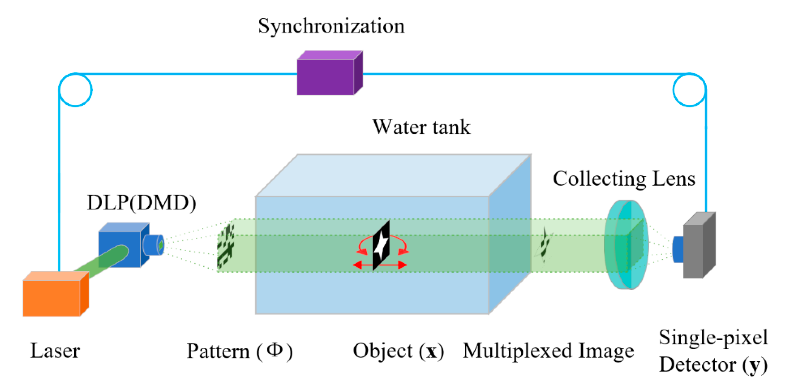
2.1. SPI Theory
2.2. LADAR Model
2.3. BRDF Reflection Model
3. Theoretical Investigation
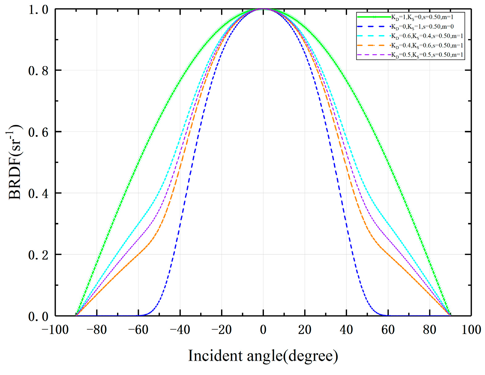
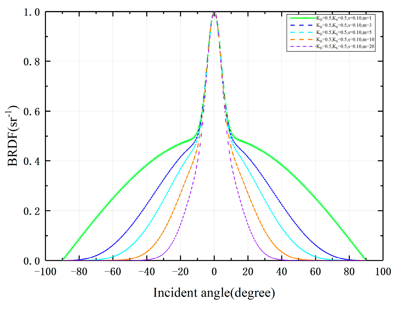
3.1. Influence of Angle of Incidence
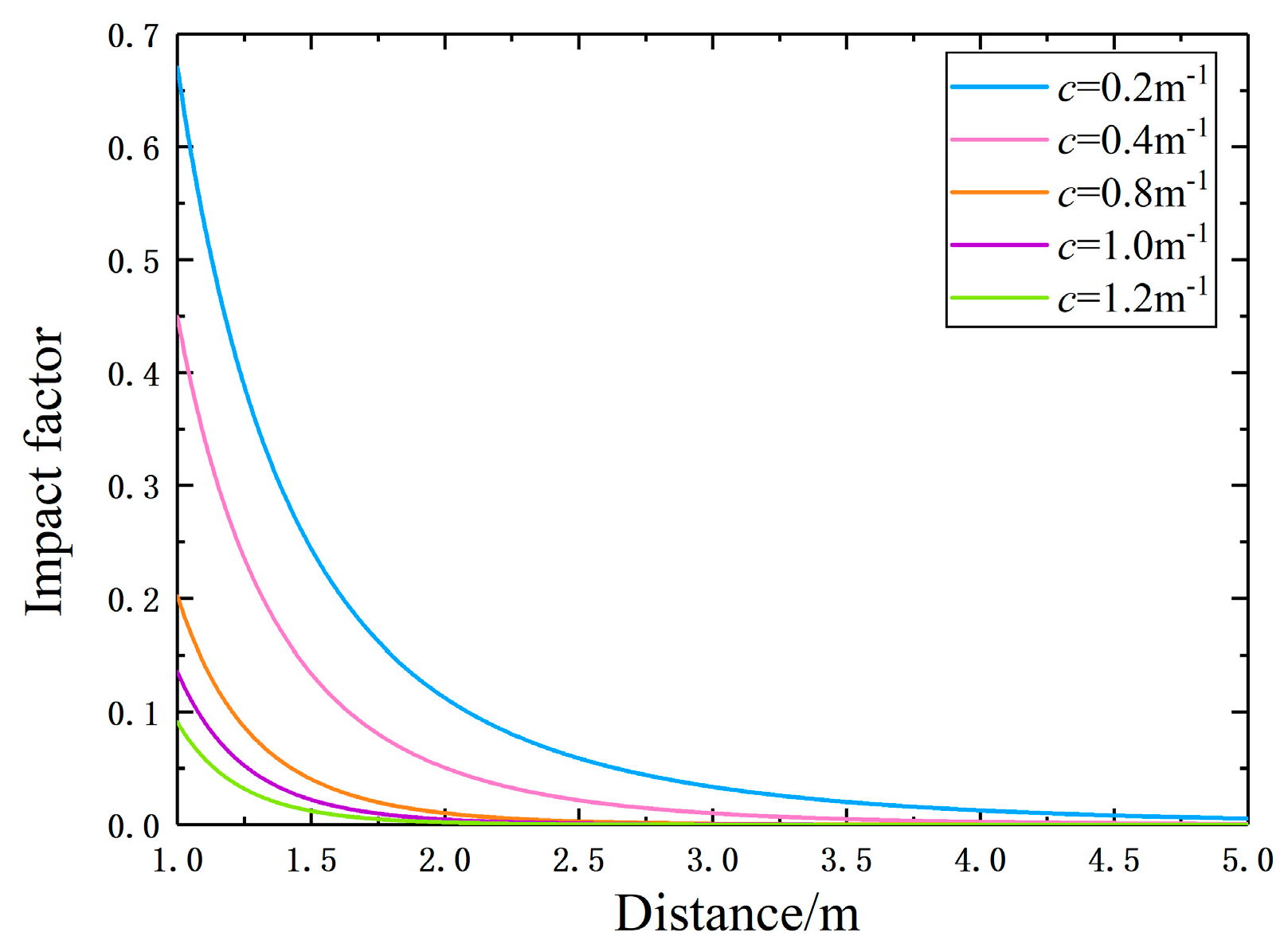
3.2. Influence of Target Distance and Medium Attenuation
4. Experimental Investigation
5. Results and Analysis
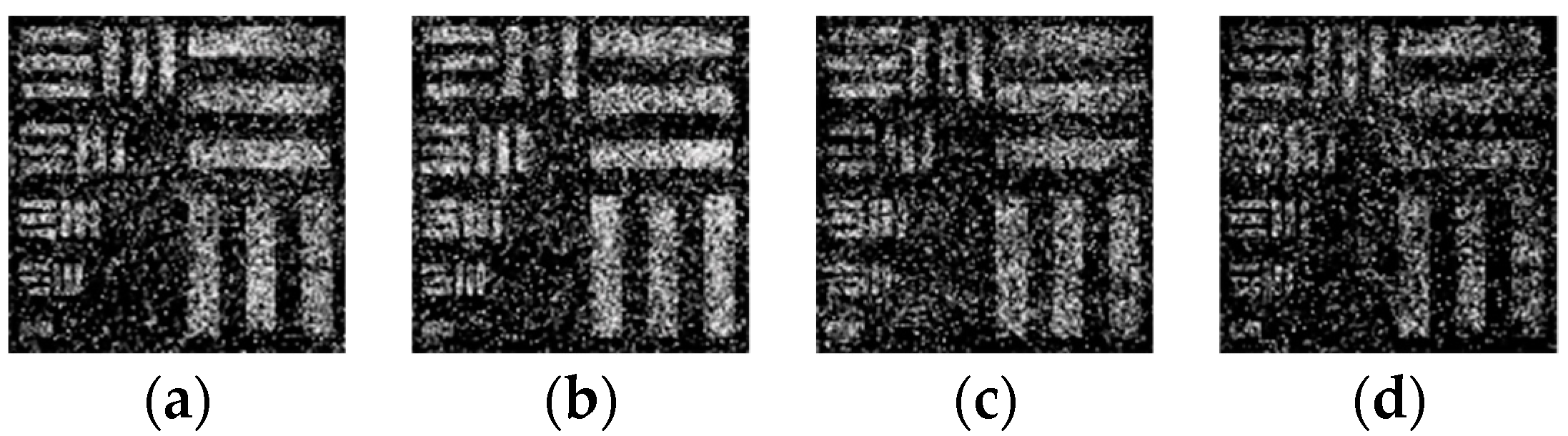
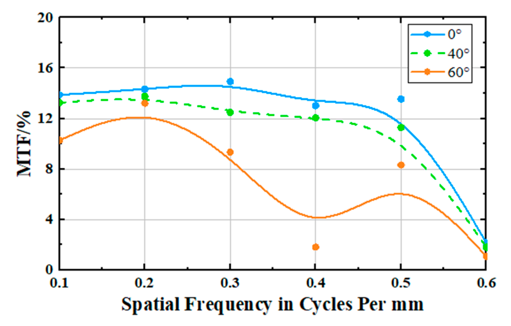
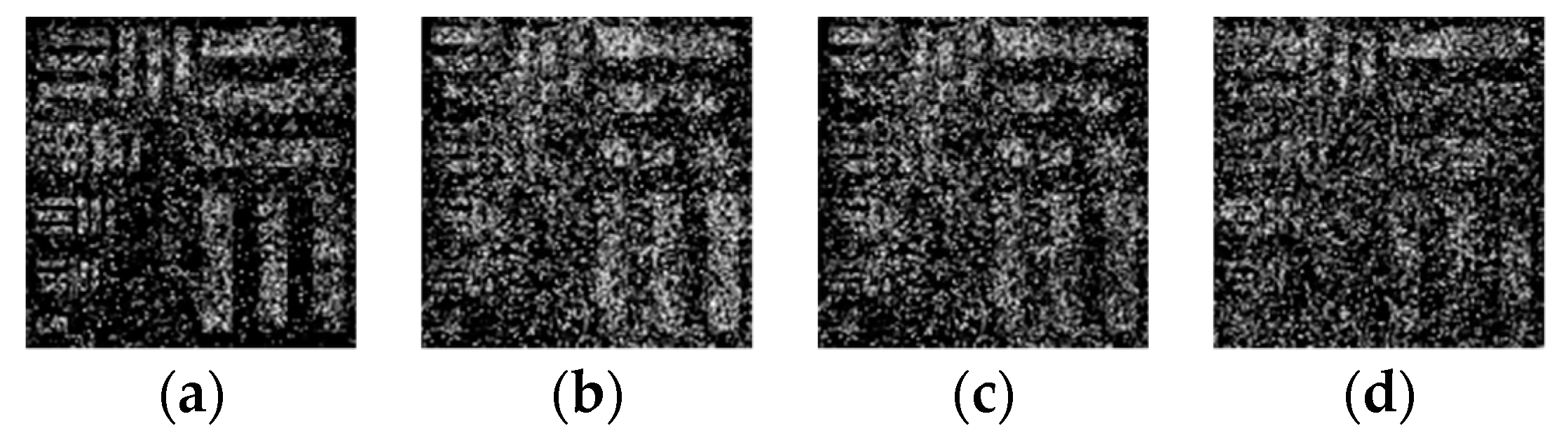
5.1. Influence of Angle of Incidence
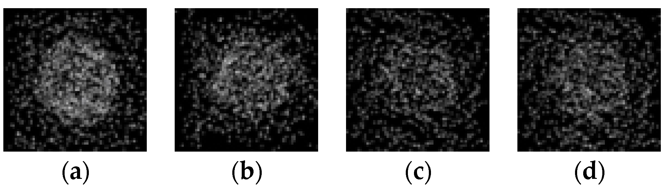
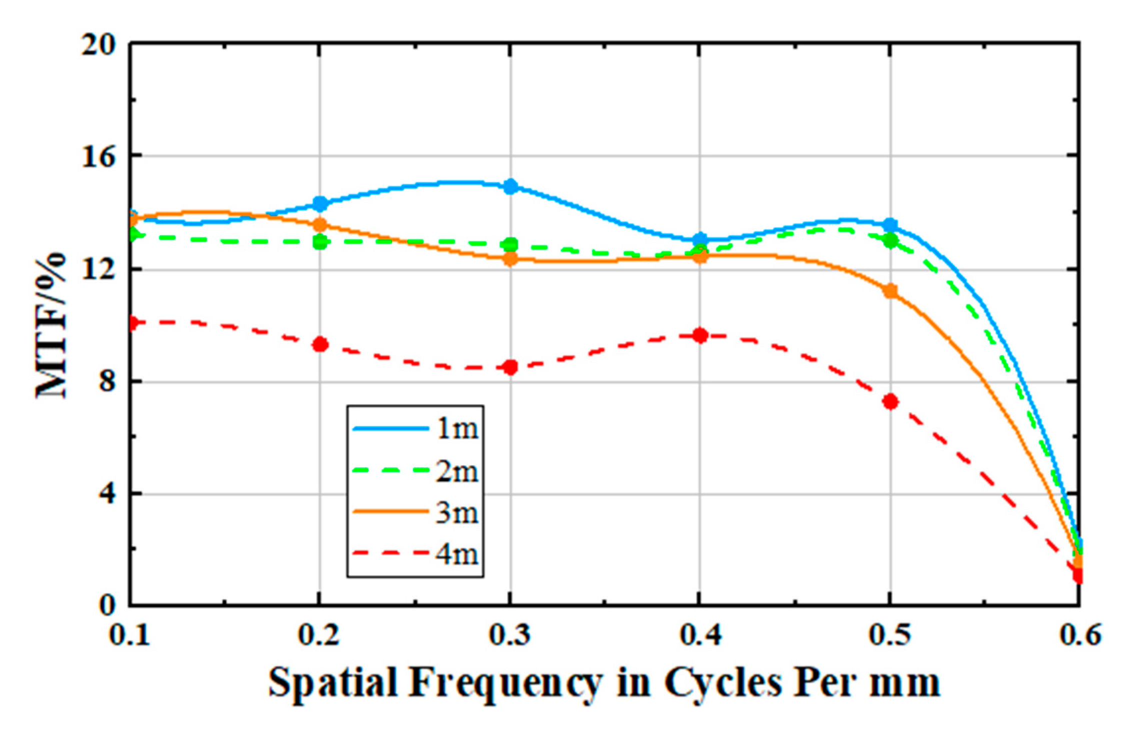
5.2. Influence of Target Distance
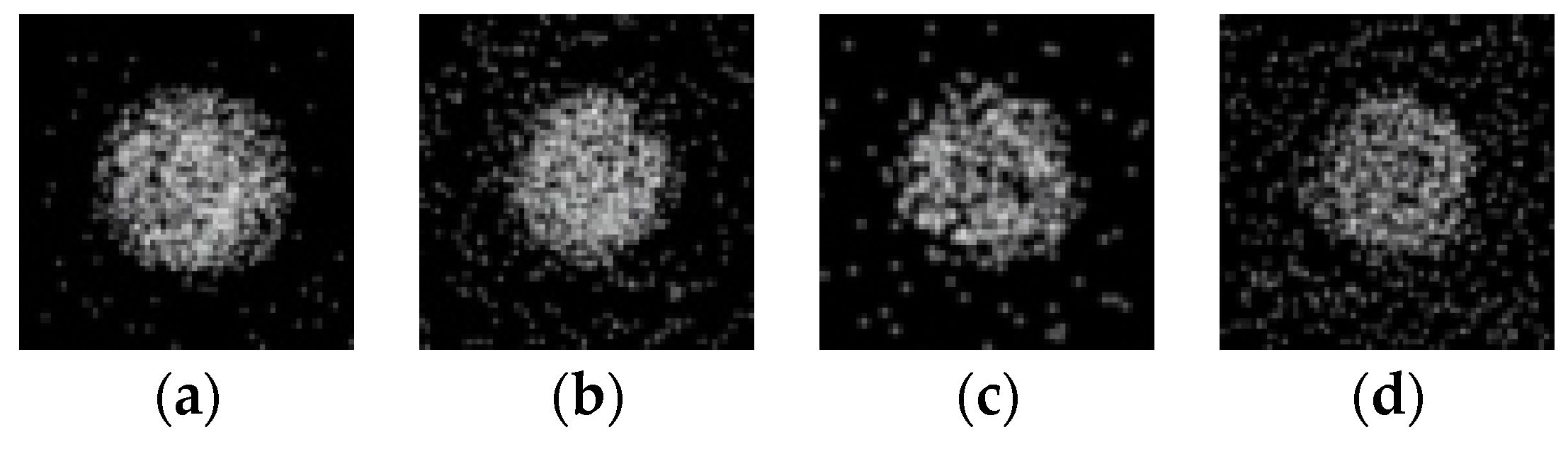
5.3. Influence of Medium Attenuation
6. Conclusions
Author Contributions
Funding
Conflicts of Interest
References
- Wang, N.; Zheng, B.; Zheng, H.; Yu, Z. Feeble object detection of underwater images through LSR with delay loop. Opt. Express 2017, 25, 22490–22498. [Google Scholar] [CrossRef]
- Sivčev, S.; Rossi, M.; Coleman, J.; Omerdić, E.; Dooly, G.; Toal, D. Collision Detection for Underwater ROV Manipulator Systems. Sensors 2018, 18, 1117. [Google Scholar] [CrossRef] [PubMed]
- Le, M.; Wang, G.; Zheng, H.; Liu, J.; Zhou, Y.; Xu, Z. Underwater computational ghost imaging. Opt. Express 2017, 25, 22859–22868. [Google Scholar] [CrossRef] [PubMed]
- Han, P.L.; Liu, F.; Zhang, G.; Tao, Y.; Shao, X.P. Multi-scale analysis method of underwater polarization imaging. Acta Phys. Sin. 2018, 67, 054202. [Google Scholar]
- Gholami, A.; Saghafifar, H. Simulation of an active underwater imaging through a wavy sea surface. J. Mod. Opt. 2018, 65, 1210–1218. [Google Scholar] [CrossRef]
- Wu, T.C.; Chi, Y.C.; Wang, H.Y.; Tsai, C.T.; Lin, G.R. Blue Laser Diode Enables Underwater Communication at 12.4 Gbps. Sci. Rep. 2017, 7, 40480. [Google Scholar] [CrossRef]
- Vidvans, A.; Basu, S. Smartphone based scalable reverse engineering by digital image correlation. Opt. Lasers Eng. 2018, 102, 126–135. [Google Scholar] [CrossRef]
- Lee, J.; Lee, K.; Lee, S.; Kim, S.W.; Kim, Y.J. High precision laser ranging by time-of-flight measurement of femtosecond pulses. Meas. Sci. Technol. 2012, 23, 207. [Google Scholar] [CrossRef]
- Amann, M.C.; Myllylae, R.A. Laser ranging: A critical review of unusual techniques for distance measurement. Opt. Eng. 2001, 40, 10–19. [Google Scholar]
- Huke, P.; Klattenhoff, R.; Von Kopylow, C.; Bergmann, R.B. Novel Trends in Optical Non-Destructive Testing Methods. J. Eur. Opt. Soc. Rapid Publ. 2011, 8, 1672–1675. [Google Scholar] [CrossRef]
- Lv, D.; Sun, J.F.; Li, Q.; Wang, Q. Model-based recognition of 3D articulated target using ladar range data. Appl. Opt. 2015, 54, 5382–5391. [Google Scholar] [CrossRef] [PubMed]
- Baumann, E.; Giorgetta, F.R.; Deschênes, J.D.; Swann, W.C.; Coddington, I.; Newbury, N.R. Comb-calibrated laser ranging for three-dimensional surface profiling with micrometer-level precision at a distance. Opt. Express 2014, 22, 24914–24928. [Google Scholar] [CrossRef] [PubMed]
- Mccarthy, A.; Collins, R.J.; Krichel, N.J.; Fernández, V.; Wallace, A.M.; Buller, G.S. Long-range time-of-flight scanning sensor based on high-speed time-correlated single-photon counting. Appl. Opt. 2009, 48, 6241–6251. [Google Scholar] [CrossRef] [PubMed]
- Andersson, P. Long-range three-dimensional imaging using range-gated laser radar images. Opt. Eng. 2006, 45, 34301. [Google Scholar] [CrossRef]
- Zevallos, L.; Manuel, E.; Gayen, S.K.; Alrubaiee, M.; Alfano, R.R. Time-gated backscattered ballistic light imaging of objects in turbid water. Appl. Phys. Lett. 2005, 86, 011113–011115. [Google Scholar] [CrossRef]
- Sluzek, A.; Chai, T.Y.; Chen, Y.F.; Tan, C.S.; Seet, G.; Wong, H.Y.; Xin, W. Scattering noise estimation of range-gated imaging system in turbid condition. Opt. Express 2010, 18, 21147–21154. [Google Scholar]
- Mullen, L.; Cochenour, B. Optical modulation techniques for underwater detection, ranging and imaging. Proc. SPIE. 2011, 8030. [Google Scholar] [CrossRef]
- Du, B.; Pang, C.; Wu, D.; Li, Z.; Peng, H.; Tao, Y.; Wu, E.; Wu, G. High-speed photon-counting laser ranging for broad range of distances. Sci. Rep. 2018, 8, 4198. [Google Scholar] [CrossRef]
- Gao, J.; Sun, J.; Wei, J.; Wang, Q. Research of underwater target detection using a Slit Streak Tube Imaging Lidar. In Proceedings of the Academic International Symposium on Optoelectronics and Microelectronics Technology, Harbin, China, 12–16 October 2011; pp. 240–243. [Google Scholar]
- Tan, C.; Sluzek, A.; Seet, G.; Shacklock, A. Three-dimensional Machine Vision Using Gated Imaging System: A Numerical Analysis. In Proceedings of the 2006 IEEE Conference on Robotics, Automation and Mechatronics, Bangkok, Thailand, 1–3 June 2006; pp. 1–6. [Google Scholar]
- Höfle, B.; Pfeifer, N. Correction of laser scanning intensity data: Data and model-driven approaches. ISPRS J. Photogramm. Remote Sens. 2007, 62, 415–433. [Google Scholar] [CrossRef]
- Chua, S.Y.; Wang, X.; Guo, N.; Tan, C.S. Range compensation for accurate 3D imaging system. Appl. Opt. 2016, 55, 153–158. [Google Scholar] [CrossRef]
- Wang, X.; Zhou, Y.; Liu, Y. Impact of echo broadening ef fect on active range-gated imaging. Chin. Opt. Lett. 2012, 10, 32–34. [Google Scholar]
- Xinwei, W.; Youfu, L.; Yan, Z. Triangular-range-intensity profile spatial-correlation method for 3D super-resolution range-gated imaging. Appl. Opt. 2013, 52, 7399–7406. [Google Scholar] [CrossRef] [PubMed]
- Yang, K. Analysis of MCP gain selection for underwater range-gated imaging applications based on ICCD. J. Mod. Opt. 2010, 57, 408–417. [Google Scholar]
- Wang, X.; Hu, L.; Zhi, Q.; Chen, Z.; Jin, W. Influence of range-gated intensifiers on underwater imaging system SNR. In Proceedings of the International Symposium on Photoelectronic Detection & Imaging, Beijing, China, 25–27 June 2013; p. 89120. [Google Scholar]
- Laux, A.; Jantzi, A.; Cochenour, B.; Mullen, L.; Jemison, W. Enhanced underwater ranging using an optical vortex. Opt. Express 2018, 26, 2668–2674. [Google Scholar]
- Zheng, B.; Wang, N.; Zheng, H.; Yu, Z.; Wang, J. Object extraction from underwater images through logical stochastic resonance. Opt. Lett. 2016, 41, 4967–4970. [Google Scholar] [CrossRef] [PubMed]
- Xu, J.; Song, Y.; Yu, X.; Lin, A.; Kong, M.; Han, J.; Deng, N. Underwater wireless transmission of high-speed QAM-OFDM signals using a compact red-light laser. Opt. Express 2016, 24, 8097–8109. [Google Scholar] [CrossRef] [PubMed]
- Hung, C.C.; Tsao, S.C.; Huang, K.H.; Jang, J.P.; Chang, H.K.; Dobbs, F.C. A highly sensitive underwater video system for use in turbid aquaculture ponds. Sci. Rep. 2016, 6, 31810. [Google Scholar] [CrossRef]
- Britton, W.B.; Dalgleish, F.R.; Zhuang, H. Beamforming receiver for underwater pulsed laser line scanning. In Proceedings of the Ocean Sensing and Monitoring X., Orlando, FL, USA, 25 May 2018; p. 106310. [Google Scholar]
- Duan, Y.; Song, C. Influence of Atmospheric Aerosol Backscattering on Incoherent Frequency Modulation Continuous-wave Laser Ranging in the Fog. Eng. Lett. 2017, 25, 15–21. [Google Scholar]
- Chen, Q.; Chamoli, S.K.; Yin, P.; Wang, X.; Xu, X. Imaging of hidden object using passive mode single pixel imaging with compressive sensing. Laser Phys. Lett. 2018, 15, 126201. [Google Scholar] [CrossRef]
- Lee, J.; Kim, Y.J.; Lee, K.; Lee, S.; Kim, S.W. Time-of-flight measurement with femtosecond light pulses. Nat. Photonics 2010, 4, 207. [Google Scholar] [CrossRef]
- Bender, P.L.; Currie, D.G.; Poultney, S.K.; Alley, C.O.; Dicke, R.H.; Wilkinson, D.T.; Eckhardt, D.H.; Faller, J.E.; Kaula, W.M.; Mulholland, J.D. The Lunar Laser Ranging Experiment: Accurate ranges have given a large improvement in the lunar orbit and new selenophysical information. Science 1973, 182, 229–238. [Google Scholar] [CrossRef] [PubMed]
- Friedland, S.; Li, Q.; Dan, S.; Bernal, E.A. Two Algorithms for Compressed Sensing of Sparse Tensors; Springer International Publishing: Berlin, Germany, 2015; pp. 259–281. [Google Scholar]
- Min, S.O.; Hong, J.K.; Kim, T.H.; Hong, K.H.; Kim, B.W.; Dong, J.P. Time-of-Flight Analysis of Three-Dimensional Imaging Laser Radar Using A Geiger-Mode Avalanche Photodiode. Jpn. J. Appl. Phys. 2010, 49, 026601–026606. [Google Scholar]
- Nicodemus, F.E. Directional Reflectance and Emissivity of an Opaque Surface. Appl. Opt. 1965, 4, 767–773. [Google Scholar] [CrossRef]
- Walter, B.; Marschner, S.R.; Li, H.; Torrance, K.E. Microfacet Models for Refraction through Rough Surfaces. In Proceedings of the Eurographics Symposium on Rendering Techniques, Grenoble, France, 25–27 June 2007; pp. 195–206. [Google Scholar]
- Ashikmin, M.; Shirley, P. A microfacet-based BRDF generator. In Proceedings of the Conference on Computer Graphics and Interactive Techniques, New York, NY, USA, 23–28 July 2000; pp. 65–74. [Google Scholar]
- Schlick, C. An Inexpensive BRDF Model for Physically-based Rendering. Comput. Graph. Forum 1994, 13, 233–246. [Google Scholar]
- Sun, J.; Wang, Q. 4-D image reconstruction for Streak Tube Imaging Lidar. Laser Phys. 2009, 19, 502. [Google Scholar] [CrossRef]
- Nevis, A.J. Automated processing for streak tube imaging lidar data. In Proceedings of the SPIE-The International Society for Optical Engineering, Orlando, FL, USA, 24–25 April 2003; p. 5089. [Google Scholar]
- Gelbart, A. Flash lidar based on multiple-slit streak tube imaging lidar. In Proceedings of the Laser Radar Technology and Applications VII, Orlando, FL, USA, 3–4 April 2002; pp. 9–18. [Google Scholar]
- Busck, J.; Heiselberg, H. Gated viewing and high-accuracy three-dimensional laser radar. Appl. Opt. 2004, 43, 4705–4710. [Google Scholar] [CrossRef]
- Seubert, C.M.; Nichols, M.E.; Frey, J.; Shtein, M.; Thouless, M.D. The characterization and effects of microstructure on the appearance of platelet–polymer composite coatings. J. Mater. Sci. 2016, 51, 2259–2273. [Google Scholar] [CrossRef]
- Field, J.J.; Wernsing, K.A.; Squier, J.A.; Bartels, R.A.J.J.A. Three-dimensional single-pixel imaging of incoherent light with spatiotemporally modulated illumination. J. Opt. Soc. Am. A 2018, 35, 1438–1449. [Google Scholar] [CrossRef]
- Huang, X.; Netravali, R.; Man, H.; Lawrence, V.J.S. Multi-sensor fusion of infrared and electro-optic signals for high resolution night images. Sensors 2012, 12, 10326–10338. [Google Scholar] [CrossRef]
- Dolin, L.S.J.A.O. Theory of lidar method for measurement of the modulation transfer function of water layers. Appl. Opt. 2013, 52, 199–207. [Google Scholar] [CrossRef]
- Mobley, C.; Boss, E.; Roesler, C. Ocean Optics Web Book. Available online: http://www.oceanopticsbook.info/ (accessed on 11 November 2019).


| Target Reflectance Characteristic | KD | KS | s | m |
|---|---|---|---|---|
| Completely rough | 1 | 0 | 0.5 | 0 |
| Completely smooth | 0 | 1 | 0.5 | 1 |
| KD > KS | 0.6 | 0.4 | 0.5 | 1 |
| KD < KS | 0.4 | 0.6 | 0.5 | 1 |
| KD = KS | 0.5 | 0.5 | 0.5 | 1 |
| Surface Number | KD | KS | s | m |
|---|---|---|---|---|
| 1 | 0.5 | 0.5 | 0.02 | 1 |
| 2 | 0.5 | 0.5 | 0.08 | 1 |
| 3 | 0.5 | 0.5 | 0.20 | 1 |
| 4 | 0.5 | 0.5 | 0.40 | 1 |
| 5 | 0.5 | 0.5 | 0.60 | 1 |
| Surface Number | KD | KS | s | m |
|---|---|---|---|---|
| 1 | 0.5 | 0.5 | 0.1 | 1 |
| 2 | 0.5 | 0.5 | 0.1 | 3 |
| 3 | 0.5 | 0.5 | 0.1 | 5 |
| 4 | 0.5 | 0.5 | 0.1 | 10 |
| 5 | 0.5 | 0.5 | 0.1 | 20 |
© 2019 by the authors. Licensee MDPI, Basel, Switzerland. This article is an open access article distributed under the terms and conditions of the Creative Commons Attribution (CC BY) license (http://creativecommons.org/licenses/by/4.0/).
Share and Cite
Chen, Q.; Mathai, A.; Xu, X.; Wang, X. A Study into the Effects of Factors Influencing an Underwater, Single-Pixel Imaging System’s Performance. Photonics 2019, 6, 123. https://doi.org/10.3390/photonics6040123
Chen Q, Mathai A, Xu X, Wang X. A Study into the Effects of Factors Influencing an Underwater, Single-Pixel Imaging System’s Performance. Photonics. 2019; 6(4):123. https://doi.org/10.3390/photonics6040123
Chicago/Turabian StyleChen, Qi, Anumol Mathai, Xiping Xu, and Xin Wang. 2019. "A Study into the Effects of Factors Influencing an Underwater, Single-Pixel Imaging System’s Performance" Photonics 6, no. 4: 123. https://doi.org/10.3390/photonics6040123
APA StyleChen, Q., Mathai, A., Xu, X., & Wang, X. (2019). A Study into the Effects of Factors Influencing an Underwater, Single-Pixel Imaging System’s Performance. Photonics, 6(4), 123. https://doi.org/10.3390/photonics6040123