Image Encryption and Decryption Systems Using the Jigsaw Transform and the Iterative Finite Field Cosine Transform

Abstract

We propose the use of the Jigsaw transform (JT) and the iterative cosine transform over a finite field in order to encrypt and decrypt images. The JT is a nonlinear operation that allows one to increase the security over the encrypted images by adding new keys to the encryption and decryption systems. The finite field is a finite set of integer numbers where the basic mathematical operations are performed using modular arithmetic. The finite field used in the encryption and decryption systems has an order given by the Fermat prime number 257. The iterative finite field cosine transform (FFCT) was used in our work with the purpose of obtaining images that had an uniform random distribution. We used a security key given by an image randomly generated and uniformly distributed. The JT and iterative FFCT was utilized twice in the encryption and decryption systems. The encrypted images presented a uniformly distributed histogram and the decrypted images were the same original images used as inputs in the encryption system. The resulting decrypted images had a high level of image quality in comparison to the image quality of the decrypted images obtained by the actual optical decryption systems. The proposed encryption and decryption systems have three security keys represented by two random permutations used in the JTs and one random image. The key space of the proposed encryption and decryption systems is larger. The previous features of the security system allow a better protection of the encrypted image against brute force and statistical analysis attacks.

1. Introduction

The cosine transform is a very useful mathematical tool that is used in applications of signal and optical processing, such as filtering, encryption, compression and recognition [1,2,3,4,5,6,7,8,9]. The finite fields are special mathematical structures based on integer numbers, which are used in image and video watermarking; digital data coding and decoding with detection and correction of errors in communication systems; estimation; compression; filtering and encryption of signals and images; and other applications [10,11,12,13,14,15]. The cosine transform over a finite field is known as the finite field cosine transform (FFCT), which is defined in [16]. This FFCT has been used in image encryption [17,18,19] with a high level security over the encrypted image. The decrypted images obtained for the decryption system based on the use of FFCT have a high level of image quality in comparison to the image quality of the resulting decrypted images in several optical decryption systems, because the FFCT over a finite field have no rounding and overflow problems [20,21,22]. Another advantage of the FFCT for the encryption system is based on the histogram uniformization of this FFCT over the image to transform [17,18].

In this work, we propose an image encryption–decryption system based on the Jigsaw transform (JT) and the iterative cosine transform over a finite field (FFCT). We use the iterative FFCT twice in order to obtain an encrypted image with an uniform histogram. The JT is a nonlinear operation, which allows a random reposition of the pixels of the image [23,24]. The JT adds new security keys to the encryption system that improve the security of the encrypted image. The encrypted image is protected by using three security keys given by two random permutations of the JTs and one random image code. Finally, we show that the proposed encryption–decryption system is resistant to brute force, statistical, entropy and differential attacks.

The retrieved decrypted images for the security systems of [23,24] are not exactly the same original images that were initially encrypted, because the mathematical operations of these security systems are computed over the real numbers. We avoid this drawback by computing the mathematical operations of the proposed encryption and decryption systems over positive integers given by finite fields, which do not introduce rounding and overflow problems in the results of the encrypted and decrypted images. The encryption systems proposed in [17,18,19] use the iterative FFCT with just one security key, whereas the encryption system of this work uses three security keys, and thus, the key space of our encryption system is larger. The image encryption algorithms of [17,18] process the original image to encrypt by dividing the image into small blocks which are overlapping. These small blocks with overlaps do not allow processing the image for encryption by using parallel computing. For the encryption system proposed in this work, the image is divided into small blocks that are not overlapping, and hence, parallel computing could be used in our encryption algorithm.

The rest of the paper is organized as follows: Section 2 introduces the mathematical background related to the JT and FFCT. In Section 3, the proposed image encryption–decryption system based on JT and FFCT is developed. Numerical simulations are computed in order to validate and verify the security system in Section 4. Finally, the main ideas of the paper are summarized in Section 5.

2. Mathematical Background

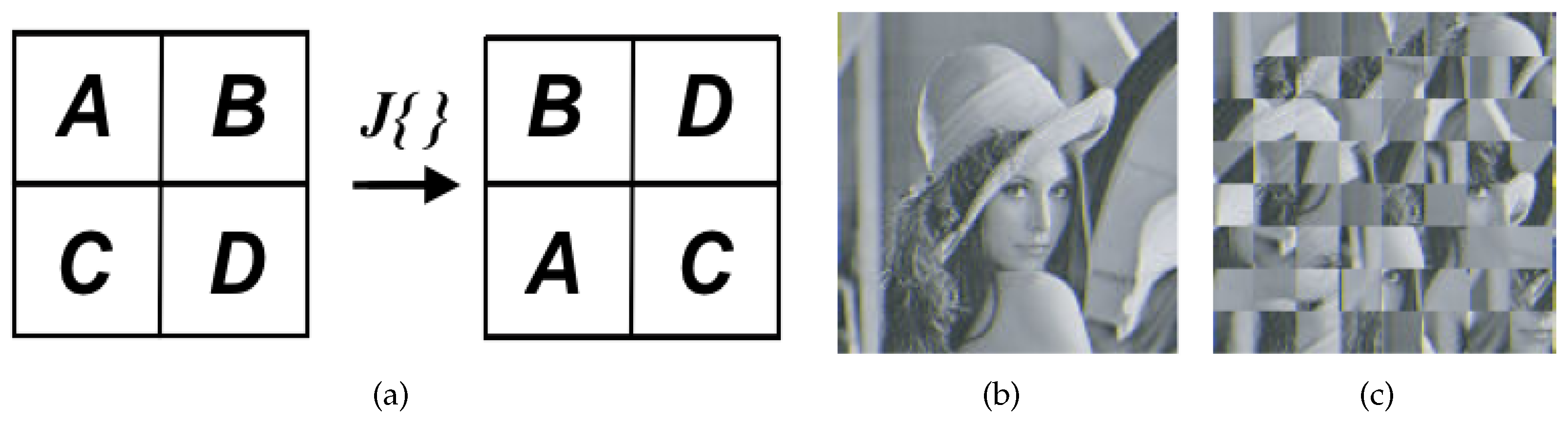
2.1. Jigsaw Transform (JT)

The Jigsaw transform, $J\{\}$, is a nonlinear operator that can be defined as a juxtaposition of different sections of an image [23,24]. A simple two-dimensional case is presented in Figure 1a. The result of the JT applied over an image (Figure 1b) is depicted in Figure 1c.

For the result of the previous figure, the image was divided into 64 subsections of 8 × 8 pixels, which were repositioned relative to each other according to some permutation. The permutation used is random. The Jigsaw transform is unitary energy conserved throughout the transform, and it also has an inverse. In the case shown in Figure 1c, there are 64! possible permutations for the JT. Each particular Jigsaw transform is denoted by some index, e.g., $J_b\{\}$, and its inverse is denoted by $J_{-b}\{\}$.

2.2. Finite Field Cosine Transform (FFCT)

The finite field is a finite set of integer numbers where the basic math operations are performed using modular arithmetic. The finite set of a finite field is represented by $Z_p=\{0,1,2,\dots ,p-1\}$ (where p is a prime number). The number of elements or the order of $Z_p$ is p. The arithmetic operation over $Z_p$ are computed modulo p [10,16].

Let $\gamma$ be an element of $Z_p$ with a multiplicative order of $2N$, then the cosine transform over the finite field $Z_p$ of the sequence or vector $x=(x_i)$, where $x_i\in Z_p$ and $i=0,1,2,\dots ,N-1$, is the sequence or vector $X=(X_k)$, where $X_k\in Z_p$ and $k=0,1,2,\dots ,N-1$, given by [16]

$$\begin{array}{c}\hfill X_k=CT\{x_i\}=\sum _{i=0}^{N-1}\sqrt{\frac{2}{N}}{\beta }_k{x}_i{cos}_{\gamma }\left(k\left(i+\frac{1}{2}\right)\right),{cos}_{\gamma }(x)=\frac{{\gamma }^x+{\gamma }^{-x}}{2},\end{array}$$

(1)

where $CT$ denotes cosine transform and $x=k(i+\frac{1}{2})$ and ${\beta }_k$ are equal to $\sqrt{2^{-1}}(\mathrm{mod}p)$ when $k=0$ and 1 for $k\ne 0$. The inverse cosine transform over the finite field $Z_p$ of the vector $X_k$ is defined by

$$\begin{array}{c}\hfill x_i=C{T}^{-1}\{X_k\}=\sum _{k=0}^{N-1}\sqrt{\frac{2}{N}}{\beta }_i{X}_k{cos}_{\gamma }\left(i\left(k+\frac{1}{2}\right)\right),\end{array}$$

(2)

where ${\beta }_i$ is equal to $\sqrt{2^{-1}}(\mathrm{mod}p)$ when $i=0$ and 1 for $i\ne 0$.

The previous forward and inverse finite field cosine transforms (FFCTs) are unitary. The forward and inverse FFCTs can be computed by using a multiplication between a matrix of size $N\times N$ and a vector with a size of $N\times 1$

$$\begin{array}{c}\hfill X_k=C\ast x_i,x_i=C^{-1}\ast X_k,\end{array}$$

(3)

where the matrices C and $C^{-1}$ of size $N\times N$, are represented by

$$\begin{array}{c}\hfill C=\sqrt{\frac{2}{N}}{\beta }_k{cos}_{\gamma }\left(k\left(i+\frac{1}{2}\right)\right),C^{-1}=\sqrt{\frac{2}{N}}{\beta }_i{cos}_{\gamma }\left(i\left(k+\frac{1}{2}\right)\right),\end{array}$$

(4)

where $i,k=0,1,2,\dots ,N-1$. The two-dimensional forward and inverse FFCT of a matrix m and M with a size of $N\times N$, respectively, can be computed by using the following matrix multiplication [17]:

$$\begin{array}{c}\hfill M=CT\{m\}=C\ast m\ast C,m=C{T}^{-1}\{M\}=C^{-1}\ast M\ast C^{-1},\end{array}$$

(5)

where the matrix $C^{-1}$ corresponds to the transpose of the matrix C.

3. Image Encryption and Decryption Systems Based on JT and FFCT

The grayscale image $I(x,y)$ to encrypt has real-valued pixels and the values of these pixels are integer numbers in the interval of [0, 255]. In order to define the matrix C of the FFCT, we use the following parameters: $p=257$ and $\gamma =8$. The multiplicative order of $\gamma =8$ in $Z_p=Z_{257}$ is 16. Therefore, the matrix C of Equation (5) has a size of $8\times 8$ and it is represented by

$$\begin{array}{c}\hfill C=\left[\begin{array}{cccccccc}242& 242& 242& 242& 242& 242& 242& 242\\ 159& 137& 151& 94& 163& 106& 120& 98\\ 6& 97& 160& 251& 251& 160& 97& 6\\ 137& 163& 98& 106& 151& 159& 94& 120\\ 242& 15& 15& 242& 242& 15& 15& 242\\ 151& 98& 94& 137& 120& 163& 159& 106\\ 97& 251& 6& 160& 160& 6& 251& 97\\ 94& 106& 137& 98& 159& 120& 151& 163\end{array}\right].\end{array}$$

(6)

The result of a two-dimensional forward or inverse FFCT using the Equation (5), can have integer numbers in the interval of [0, 256]. The integer number of 256 represents an overflow for the values of the pixels of the images presented in the encryption–decryption system. Therefore, we use the iterative two-dimensional FFCT in the encryption or decryption systems in order to avoid the mentioned overflow. The iteration of the computing for the two-dimensional FFCT stops when the result of this transform has integer numbers different from 256.

In the first step of the encryption system, we divide the image $I(x,y)$ to encrypt into several subsections of $8\times 8$ pixels. We obtain the encrypted image when the following equation is applied to each subsection of the image $I(x,y)$

$$\begin{array}{c}\hfill E_s(x,y)=C{T}^{-1}\{J_b\{CT\{J_a\{I_s(x,y)\}\}\oplus K\}\},\end{array}$$

(7)

where $I_s(x,y)$ is a subsection of $I(x,y)$, $J_a$ and $J_b$ represent two JTs with two different random permutations, $CT$; $C{T}^{-1}$ and ⊕ denote the two-dimensional forward and inverse FFCT and the exclusive or operation, respectively; and K is a random image code of $8\times 8$ pixels with an uniform probability density function. The security keys of the encryption system are given by the two random permutations of the JTs and the random code image K.

The decrypted image is obtained using the following equation

$$\begin{array}{c}\hfill D_s(x,y)=J_{-a}\{C{T}^{-1}\{J_{-b}\{CT\{E_s(x,y)\}\}\oplus \widehat{K}\}\},\end{array}$$

(8)

where $J_{-a}$ and $J_{-b}$ are the inverse JTs of $J_a$ and $J_b$, respectively. The retrieved image at the output of the decryption system corresponds to the image $I(x,y)$ when the random permutations used in $J_{-a}$ and $J_{-b}$ are the same for $J_a$ and $J_b$, respectively, and $\widehat{K}=K$. If the previous conditions are provided, we will obtain $D_s(x,y)=I_s(x,y)$.

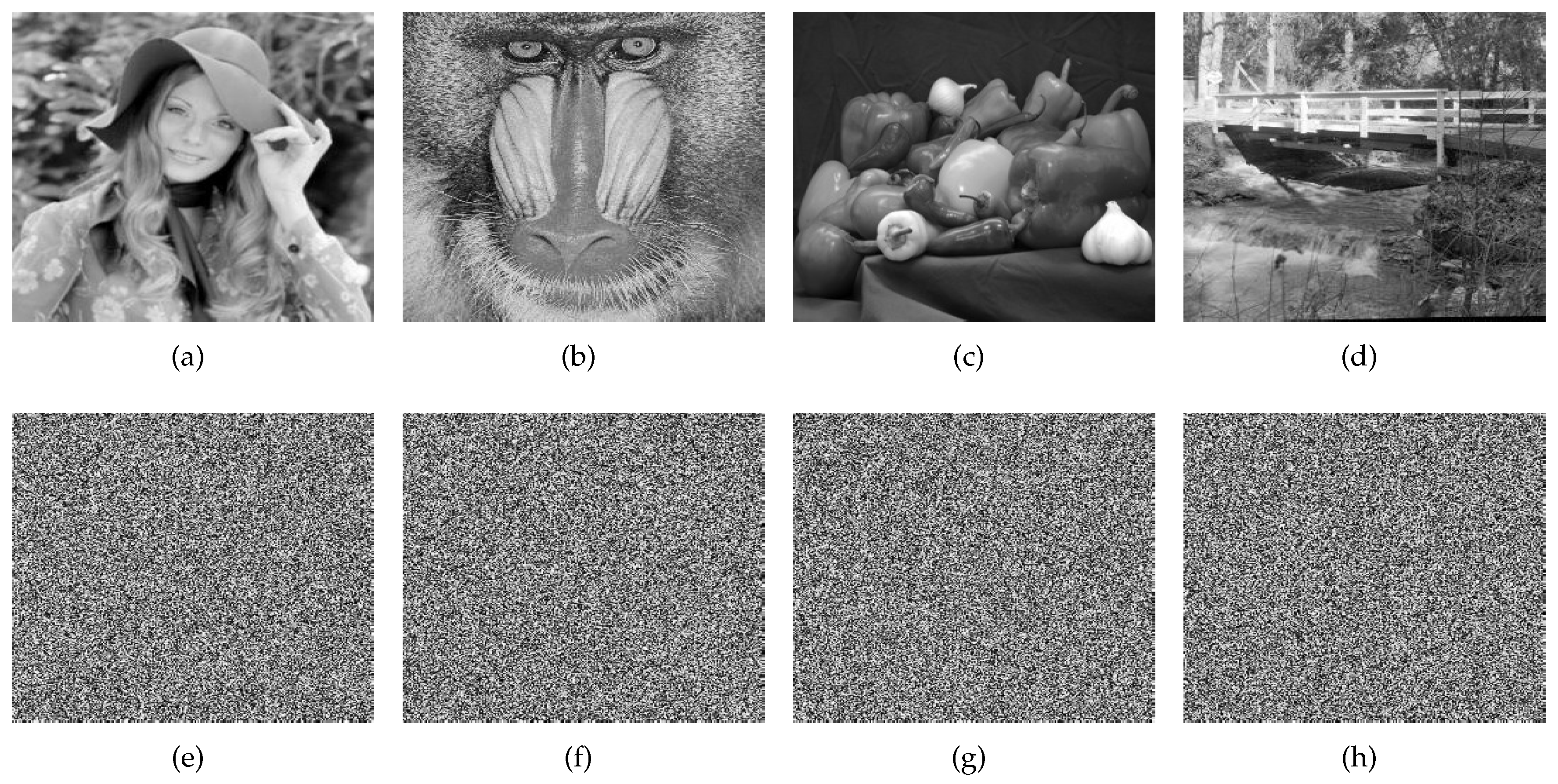
4. Numerical Experiments

The results of the numerical simulations for the encryption–decryption system proposed in Section 3 are shown in Figure 2. The images $I(x,y)$ to encrypt are depicted in Figure 2a–d. These images to encrypt have different aspects and frequencies. The resulting encrypted images $E(x,y)$ from the images of Figure 2a–d and Equation (7) are presented in Figure 2e–h, respectively. These encrypted images are noisy images that do not reveal any information of the original images $I(x,y)$.

When the decryption system is performed using the encrypted images of Figure 2e–h, the three correct security keys (the two random permutations of the JTs and the random code image K) and Equation (8), the original images $I(x_{,}y)$ of Figure 2a–d, respectively, are retrieved at the output of the decryption system. Therefore, the metric of the root mean square error (RMSE) between the decrypted images and the original images is always zero provided that the security keys used in the decryption system are the same used in the encryption system. If wrong values of the three security keys are used in the decryption system, the resulting decrypted image will be a noisy image very similar to the one shown in Figure 2e.

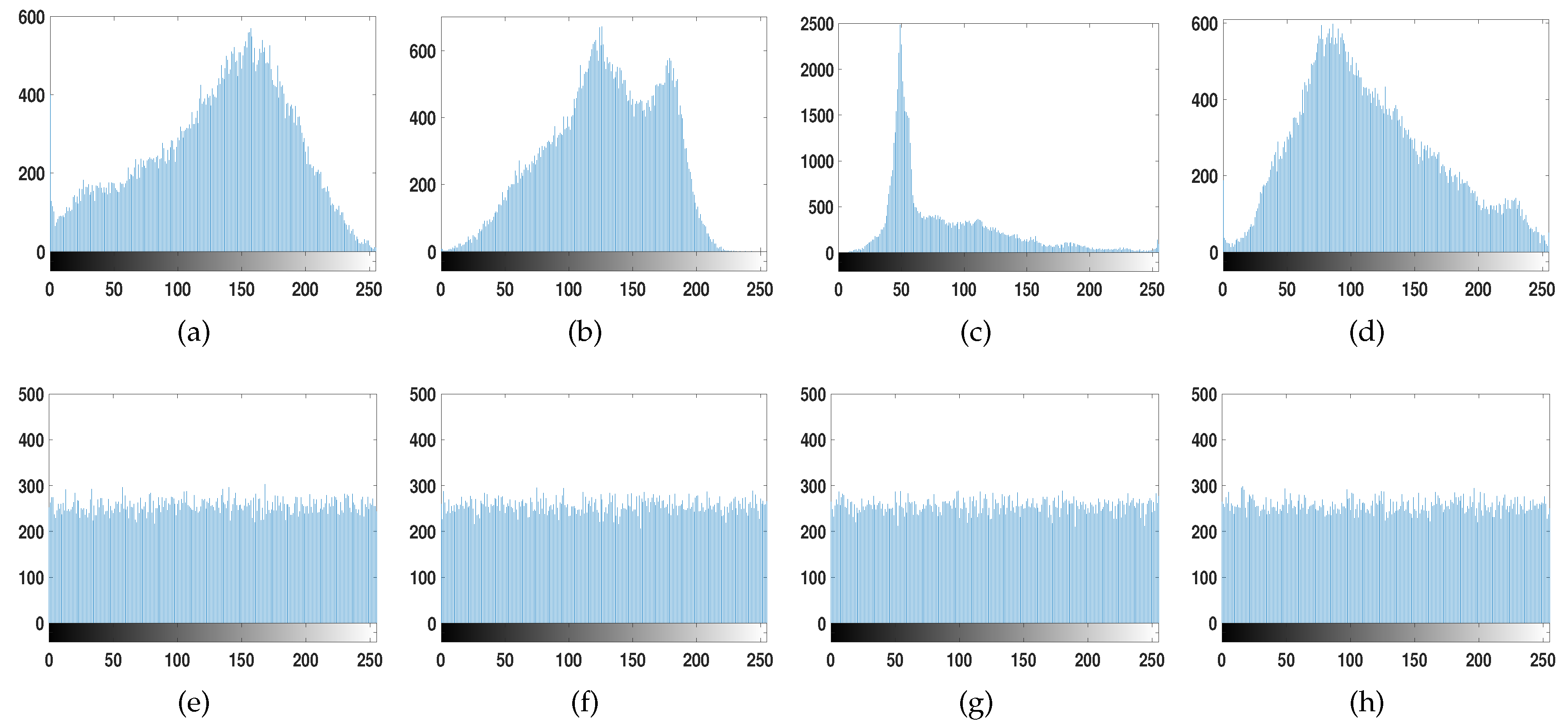
4.1. Statistical Analysis

In Figure 3a–d, we present the histograms for the original images $I(x_{,}y)$ of Figure 2a–d, respectively. These histograms confirm that the original images have different details and frequencies. The histograms for the encrypted images $E(x_{,}y)$ of Figure 2e–h are shown in Figure 3e–h, respectively. These last histograms show that the encrypted images are close to a random distribution with an uniform probability density function. The histograms of the encrypted images demonstrate that the proposed encryption system has an excellent property of diffusion for the encrypted images with respect to the different types of original images. This new feature allows an improved resistance of the proposed encryption–decryption system against statistical attacks.

The correlation distributions for the original image of Figure 2a and the encrypted image of Figure 2e are shown in Figure 4a,b, respectively. The correlation was computed between two adjacent pixels, and the two adjacent pixels were randomly chosen in the horizontal direction. Similar distributions were obtained for other images and directions in pixel adjacency. The Figure 4a shows a strong correlation between the adjacent pixels in the horizontal direction for the original image of Figure 2a, while the Figure 4b presents a weak correlation between the adjacent pixels in the horizontal direction for the encrypted image of Figure 2e. This result confirms again that the proposed encryption system has an excellent property of diffusion for the encrypted images with respect to the different types of original images.

4.2. Entropy Analysis

The entropy $H_q$ of an information source q is defined by [15].

$$\begin{array}{c}\hfill H_q=\sum _{i=0}^{R-1}p(q_i){log}_2\frac{1}{p(q_i)},\end{array}$$

(9)

where R is the total number of symbols $q_i$ of q and $p(q_i)$ denote the probability of occurrence of symbol $q_i$. For a random source with 256 equiprobable symbols, it has an entropy value of $H_q=8$. The entropy values for the encrypted images of this work are values varying from 7.9985 to 7.9987. These values of entropy confirm again that the encrypted images are close to a random distribution with a uniform probability density function and the proposed encryption–decryption system is resistant to the entropy attack.

4.3. Key Space

The key space of the proposed encryption–decryption system represents every possible combination of the three security keys given by the two random permutations of the JTs and the random code image K. The JTs are applied to subsections of $8\times 8$ pixels. Therefore, there are $64!$ possible random permutations for each JT applied in the encryption system. The number of possible random permutations are ${(64!)}^2$. The random image code K has a resolution of $8\times 8$ pixels and each pixel has 256 possible values. The number of attempts required to retrieve the random image code K is of the order of ${256}^{(8)(8)}={256}^{64}$. Therefore, the key space is given by the following product: ${(64!)}^2({256}^{64})$. The brute force attacks are intractable just considering all the possibilities of the three security keys of the proposed encryption–decryption system.

4.4. Differential Attack

Usually, the metrics of number of pixels change rate (NPCR) and the unified average changing intensity (UACI) are utilized in order to evaluate the resistance of an encryption system against differential attack. These metrics of NPCR and UACI allow one to compare the encrypted images obtained from two minimally different original images to be encrypted. The NPCR and UACI are defined by [15]

$$\begin{array}{c}\hfill \mathrm{NPCR}=\frac{{\sum }_{x=0}^{N-1}{\sum }_{y=0}^{N-1}D(x,y)}{N\times N}\times 100\%,\end{array}$$

(10)

$$\begin{array}{c}\hfill \mathrm{UACI}=\frac{{\sum }_{x=0}^{N-1}{\sum }_{y=0}^{N-1}|E_1(x,y)-E_2(x,y)|}{255(N\times N)},\end{array}$$

(11)

where $E_1(x,y)$ and $E_2(x,y)$ are the two encrypted images corresponding to the original images $I_1(x,y)$ and $I_2(x,y)$, respectively, that have one pixel difference; $N\times N$ is the size or resolution of the original and encrypted images; and $D(x,y)$ is equal to 1 when $E_1(x,y)\ne E_2(x,y)$ and 0 for other cases.

In order to compute the metrics of NPCR and UACI, we use the original images $I(x,y)$ presented in the first row of Figure 2. For each original image $I_1(x,y)$, we randomly choose one of its pixel and the least significant bit of this selected pixel is inverted; therefore, a new original image $I_2(x,y)$ is obtained from the original image $I_1(x,y)$. Now, the original images $I_1(x,y)$ and $I_2(x,y)$ are encrypted using the same three security keys (the two random permutations of the JTs and the random code image K) and the resulting encrypted images are $E_1(x,y)$ and $E_2(x,y)$, respectively. Then, the values for the metrics of NPCR and UACI are computed. These operations are computed one thousand times for each original image shown in the first row of Figure 2. The computed NPCR and UACI values vary from 99.56% to 99.67% and 33.37% to 33.61%, respectively. The values of the NPCR near to 100% and the UACI greater than 33.3% confirm that a very small change in an original image leads to a considerable change in the encrypted image. Therefore, the proposed encryption–decryption system is resistant to differential attack.

4.5. Key Sensitivity

In order to study the key sensitivity for the three security keys (the two random permutations of the JTs and the random code image K) of the proposed encryption and decryption systems, we evaluate the differences between the original image to be encrypted and the decrypted image obtained with a key minimally different from the correct one. First, we encrypt an original image using three given security key, and then, we use this encrypted image in the decryption system using two correct security keys and the third key with a small error. For each security key represented by the two random permutations of the JTs, we permute two positions of this security key with the purpose of obtaining an incorrect security key for the decryption system. The difference between the original image and the decrypted image obtained with the wrong security key is computed using the metric of the NPCR presented in Equation (10). When we use one incorrect random permutation of the JT in the decryption system, the other random permutation used in the another JT and the random code image K are correct. The resulting NPCR values vary from 99.52% to 99.65%, these results show that the proposed encryption and decryption system is highly sensitive to small changes in the security keys given by the two random permutations of the JTs.

The key sensitivity for the the random code image K is evaluated in a similar way as the two random permutations of the JTs. To generate a wrong key of the random code image K to use in the decryption system, we randomly choose one pixel of image K and the least significant bit of this chosen pixel is inverted. The image K is a random code of 8 × 8 pixels. When we use a wrong random code image K in the decryption system, the two security keys given by the two random permutations of the JTs are right. Again, we compute the NPCR between the original image and the decrypted image obtained with the incorrect key of the random code image K. This procedure is performed for every pixel of image K. Therefore, the NPCR is computed 64 times and their values vary from 99.54% to 99.68%; these values of the NPCR, close to 100%, also show that the proposed encryption and decryption system is highly sensitive to small changes in the security key given by the random code image K.

4.6. Computing Time

Using a typical, modern office computer with an Intel Core i7 of 2.7 GHz CPU, 4 GB RAM, operating system Windows 10 and the numerical computation platform Matlab, we evaluated the computing time for the proposed encryption and decryption systems. The encryption and decryption system performed the same computations. The encryption system computed two iterative FFCTs, one direct and the another inverse; two direct JTs; and the exclusive or operation over 64 pair of pixels. For the decryption system the two direct JTs are replaced by two inverse JTs with the same number of operations. The major computing time for the encryption system is due to the computation of the iterative FFCT, because the JT and the exclusive or operation are faster operations. The average computation time obtained in our simulation for an two-dimensional iterative FFCT of a matrix or image subsection $I_s(x,y)$ with a size of 8 × 8 pixels was 14 µs. For an original image of 1024 × 1024 pixels, the number of image subsections with a size of 8 × 8 pixels are 16,384 and the computing times for the proposed encryption and decryption systems are 0.487 and 0.486 s, respectively, whenever the iterative FFCTs of the 16,384 image subsections will be computed in a serial manner. Finally, the computing time of the proposed encryption and decryption system can be increased by using parallel computing and fast algorithms to compute the FFCTs.

5. Conclusions

We have presented an image encryption–decryption system based on the JT and the iterative FFCT. We showed that the proposed security system is resistant to statistical, entropy, brute force and differential attacks. The encrypted images have close to a random distribution with an uniform probability density function due to the use of the iterative FFCT. The encrypted image was protected by using three security keys represented by the two random permutations of the JTs and the random code image K. The use of JT allowed us to increase the security over the encrypted images by adding two keys to the encryption and decryption systems. The decrypted image we retrieved was the same original image that was used as input in the encryption system. The decrypted image presented a high level of image quality because of using the cosine transform over a finite field.

References

1. Gu, Z.H.; Leger, J.R.; Lee, S.H. Optical computations of cosine transforms. Opt. Commun. 1981, 39, 137–142. [Google Scholar] [CrossRef]
2. Goodman, J.W. Introduction to Fourier Optics; McGraw-Hill: New York, NY, USA, 1996. [Google Scholar]
3. Ozaktas, H.M.; Zalevsky, Z.; Kutay, M.A. The Fractional Fourier Transform: With Applications in Optics and Signal Processing; Wiley: Hoboken, NJ, USA, 2001. [Google Scholar]
4. Rao, K.; Yip, P. Discrete Cosine Transform: Algorithms, Advantages, Applications; Academic Press: San Diego, CA, USA, 2014. [Google Scholar]
5. Krikor, L.; Baba, S.; Arif, T.; Shaaban, Z. Image encryption using DCT and stream cipher. Eur. J. Sci. Res. 2009, 32, 47–57. [Google Scholar]
6. Liu, Z.; Xu, L.; Liu, T.; Chen, H.; Li, P.; Lin, C.; Liu, S. Color image encryption by using Arnold transform and color-blend operation in discrete cosine transform domains. Opt. Commun. 2011, 284, 123–128. [Google Scholar] [CrossRef]
7. Pan, S.M.; Wen, R.H.; Zhou, Z.H.; Zhou, N.R. Optical multi-image encryption scheme based on discrete cosine transform and nonlinear fractional Mellin transform. Multimed. Tools Appl. 2017, 76, 2933–2953. [Google Scholar] [CrossRef]
8. Hua, Z.; Zhou, Y.; Huang, H. Cosine-transform-based chaotic system for image encryption. Inf. Sci. 2019, 480, 403–419. [Google Scholar] [CrossRef]
9. Kumar, S.; Panna, B.; Jha, R.K. Medical image encryption using fractional discrete cosine transform with chaotic function. Med. Biol. Eng. Comput. 2019, 57, 2517–2533. [Google Scholar] [CrossRef] [PubMed]
10. Schroeder, M. Number Theory in Science and Communication: With Applications in Cryptography, Physics, Digital Information, Computing, and Self-Similarity; Springer: Berlin, Germany, 2009. [Google Scholar]
11. Bhattacharya, M.; Creutzburg, R.; Astola, J. Some historical notes on number theoretic transform. In Proceedings of the International TICS Workshop on Spectral Methods and Multirate Signal Processing, Vienna, Austria, 11–12 September 2004. [Google Scholar]
12. Abdallah, E.E.; Hamza, A.B.; Bhattacharya, P. MPEG video watermarking using tensor singular value decomposition. In Proceedings of the International Conference Image Analysis and Recognition, Montreal, QC, Canada, 22–24 August 2007. [Google Scholar]
13. Abdallah, E.E.; Hamza, A.B.; Bhattacharya, P. Video watermarking using wavelet transform and tensor algebra. Signal Image Video Process. 2010, 4, 233–245. [Google Scholar] [CrossRef]
14. Stoyanov, B.; Kordov, K. Novel image encryption scheme based on Chebyshev polynomial and duffing map. Sci. World J. 2014, 2014, 283639. [Google Scholar] [CrossRef] [PubMed]
15. Stoyanov, B.; Kordov, K. Image encryption using Chebyshev map and rotation equation. Entropy 2015, 17, 2117–2139. [Google Scholar] [CrossRef]
16. Lima, J.B.; de Souza, R.M.C. Finite field trigonometric transforms. Appl. Algebr. Eng. Commun. 2011, 22, 393–411. [Google Scholar] [CrossRef]
17. Lima, J.; Lima, E.; Madeiro, F. Image encryption based on the finite field cosine transform. Signal Process. Image Commun. 2013, 28, 1537–1547. [Google Scholar] [CrossRef]
18. Lima, J.; Madeiro, F.; Sales, F. Encryption of medical images based on the cosine number transform. Signal Process. Image Commun. 2015, 35, 1–8. [Google Scholar] [CrossRef]
19. Mikhail, M.; Abouelseoud, Y.; ElKobrosy, G. Two-phase image encryption scheme based on FFCT and fractals. Secur. Commun. Netw. 2017, 2017, 7367518. [Google Scholar] [CrossRef]
20. Millán, M.S.; Pérez-Cabré, E. Optical data encryption. In Optical and Digital Image Processing: Fundamentals and Applications; Cristóbal, G., Schelkens, P., Thienpont, H., Eds.; Wiley-VCH Verlag GmbH & Co.: Hoboken, NJ, USA, 2011; pp. 739–767. [Google Scholar]
21. Millán, M.S.; Pérez-Cabré, E.; Vilardy, J.M. Nonlinear techniques for secure optical encryption and multifactor authentication. In Advanced Secure Optical Image Processing for Communications; Al Falou, A., Ed.; IOP Publishing: Bristol, UK, 2018; pp. 8-1–8-33. [Google Scholar]
22. Muniraj, I.; Sheridan, J.T. Optical Encryption and Decryption; SPIE: Bellingham, WA, USA, 2019. [Google Scholar]
23. Hennelly, B.; Sheridan, J.T. Optical image encryption by random shifting in fractional Fourier domains. Opt. Lett. 2003, 28, 269–271. [Google Scholar] [CrossRef] [Green Version]
24. Vilardy, J.M.; Torres, C.O.; Mattos, L. Image encryption-decryption system based on Gyrator transform and Jigsaw transform. Proc. SPIE 2013, 8785, 87851Q. [Google Scholar]
Figure 1. (a) Graphical effect of the Jigsaw transform (JT). (b) Input image of the JT with a resolution of 256 × 256 pixels in grayscale. (c) Input image after the first 16 × 16 Jigsaw transforms.
Photonics 06 00121 g001
Figure 2. Original images to encrypt I ( x , y ) : (a) woman wearing a hat, (b) mandrill, (c) peppers and (d) a bridge. Encrypted images E ( x , y ) obtained from the images of: (e) Figure 2a, (f) Figure 2b, (g) Figure 2c and (h) Figure 2d.
Photonics 06 00121 g002
Figure 3. Histograms of the original images to encrypt I ( x , y ) obtained from the images of: (a) Figure 2a, (b) Figure 2b, (c) Figure 2c and (d) Figure 2d. Histograms of the encrypted images E ( x , y ) obtained from the images of: (e) Figure 2e, (f) Figure 2f, (g) Figure 2g and (h) Figure 2h.
Photonics 06 00121 g003
Figure 4. Resulting correlation distribution images for the test of correlation between two adjacent pixels applied to the image of: (a) Figure 2a, and (b) Figure 2e.
Photonics 06 00121 g004