Image-Based Laser-Beam Diagnostics Using Statistical Analysis and Machine Learning Regression

Abstract

This study is a comprehensive experimental and computational investigation into high-resolution laser beam diagnostics, combining classical statistical techniques, numerical image processing, and machine learning-based predictive modeling. A dataset of 50 sequential beam profile images was collected from a femtosecond fiber laser operating at a central wavelength of 780 nm with a pulse duration of approximately 125 fs. These images were analyzed to extract spatial and temporal beam characteristics, including centroid displacement, Full Width at Half Maximum (FWHM), ellipticity ratio, and an asymmetry index. All parameters were derived using intensity-weighted algorithms and directional cross-sectional analysis to ensure accurate and consistent quantification of the beam’s dynamic behavior. Linear regression models were applied to horizontal and vertical intensity distributions to assess long-term beam stability. The resulting predictive trends revealed a systematic drift in beam centroid position, most notably along the vertical axis, and a gradual broadening of the horizontal FWHM. The modeling further showed that vertical intensity increased over time while horizontal intensity displayed a slight decline, reinforcing the presence of axis-specific fluctuations. These effects are attributed to minor optical misalignments or thermally induced variations in the beam path. By integrating deterministic analysis with data-driven forecasting, this methodology offers a robust framework for real-time beam quality evaluation. It enhances sensitivity to subtle distortions and supports the future development of automated, self-correcting laser systems. The results underscore the critical role of continuous, high-resolution monitoring in maintaining beam stability and alignment precision in femtosecond laser applications.

1. Introduction

Laser beam profiling plays a central role in ensuring the precision and reliability of modern laser systems [1,2]. It enables detailed analysis of beam characteristics such as spatial intensity distribution, divergence, and symmetry, directly impacting performance across scientific research, industrial manufacturing, and medical diagnostics [3,4]. Even minor deviations in beam properties can lead to significant inefficiencies, reduced accuracy, and inconsistency in high-precision applications [5,6,7]. Conventional diagnostic techniques, including direct imaging, Gaussian fitting, and basic intensity distribution mapping, offer foundational insights but often fall short when detecting complex or evolving distortions within the beam. These methods typically lack the temporal resolution or adaptability required to identify alignment drifts, thermal effects, or mechanical instabilities that may occur over time. A more robust assessment involving parameters such as centroid displacement, beam symmetry, and full-width at half maximum (FWHM) variation is essential for achieving consistent and optimal system performance [8].

A range of established approaches have been used for beam quality evaluation, including knife-edge scanning [9], Hartmann–Shack wavefront sensing [10,11], and optical resonator-based Gaussian fitting methods [12]. While these techniques effectively measure static profiles and general propagation parameters, they often struggle to capture real-time beam dynamics or diagnose fine-scale temporal fluctuations. For instance, while cross-sectional intensity analysis can characterize beam shape, it offers limited insight into how it evolves due to misalignment or environmental changes [13]. Similarly, centroid tracking provides a measure of beam stability, but, in isolation, it cannot uncover systematic patterns in beam movement over time. Image processing methods such as edge detection and thresholding have also been applied [14], but they tend to lack the robustness needed for adaptive, real-time analysis.

This study introduces a comprehensive diagnostic framework that integrates traditional statistical analysis with numerical modeling techniques to address these limitations. A dataset of 50 laser-beam profile images was processed using a combination of centroid tracking, FWHM evaluation, and asymmetry analysis. Crucially, we also incorporated linear regression modeling to detect trends and predict beam fluctuations, a method that moves beyond single-frame analysis to evaluate beam behavior across an entire sequence. Our study is distinct in its structured, data-driven approach to analyzing laser beam behavior using a complete sequence of experimentally recorded beam-profile images. Rather than relying on isolated snapshots or manually selected metrics, we apply a unified analysis to the entire dataset, allowing for the extraction of key spatial and temporal parameters across all frames. By incorporating predictive modeling alongside statistical and numerical techniques, we provide a more complete and insightful evaluation of beam characteristics. This method offers consistency, objectivity, and depth, often lacking in conventional, frame-by-frame analysis, and serves as a foundation for future developments in scalable and intelligent laser diagnostics [15].

2. Methodology

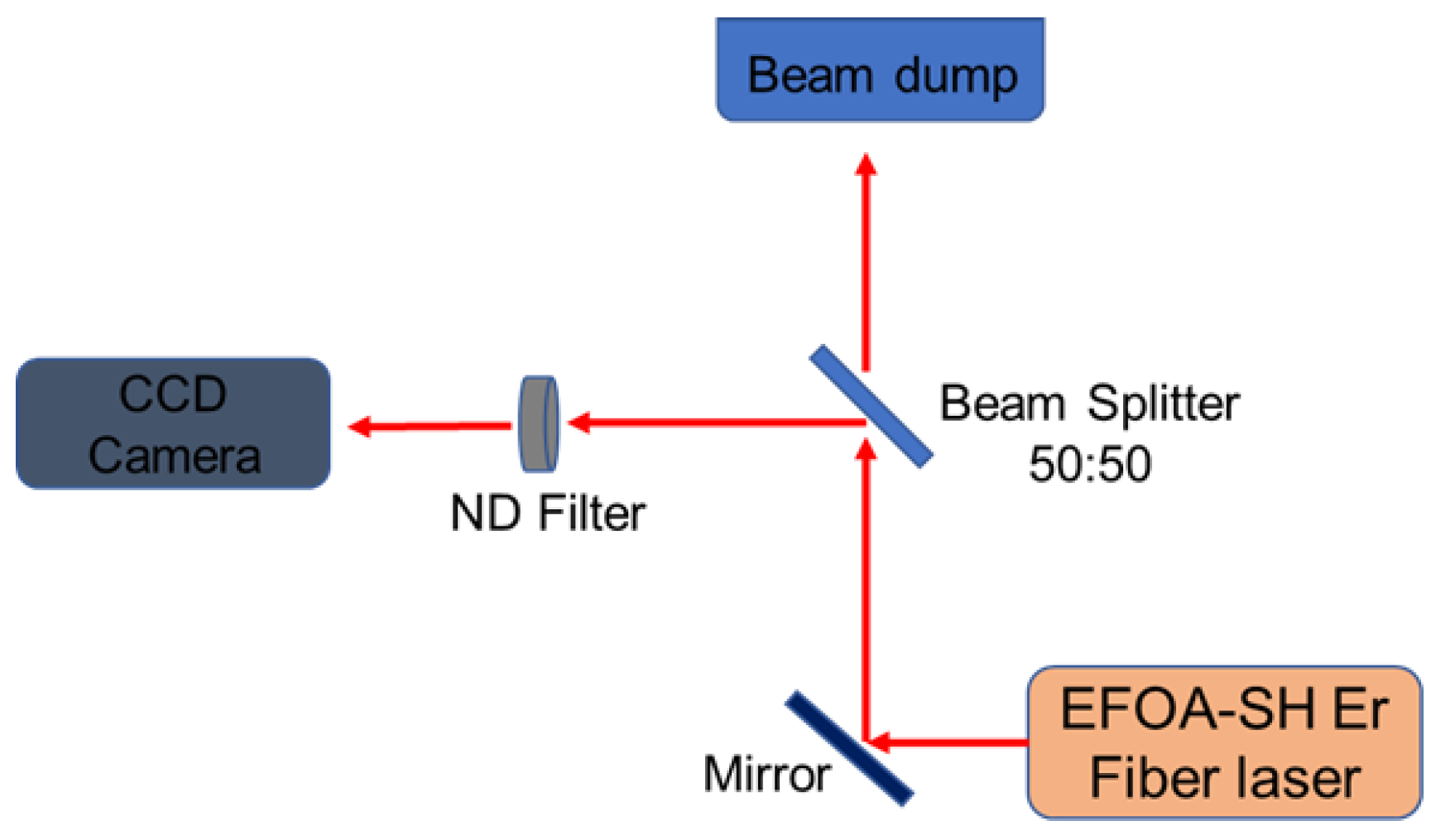
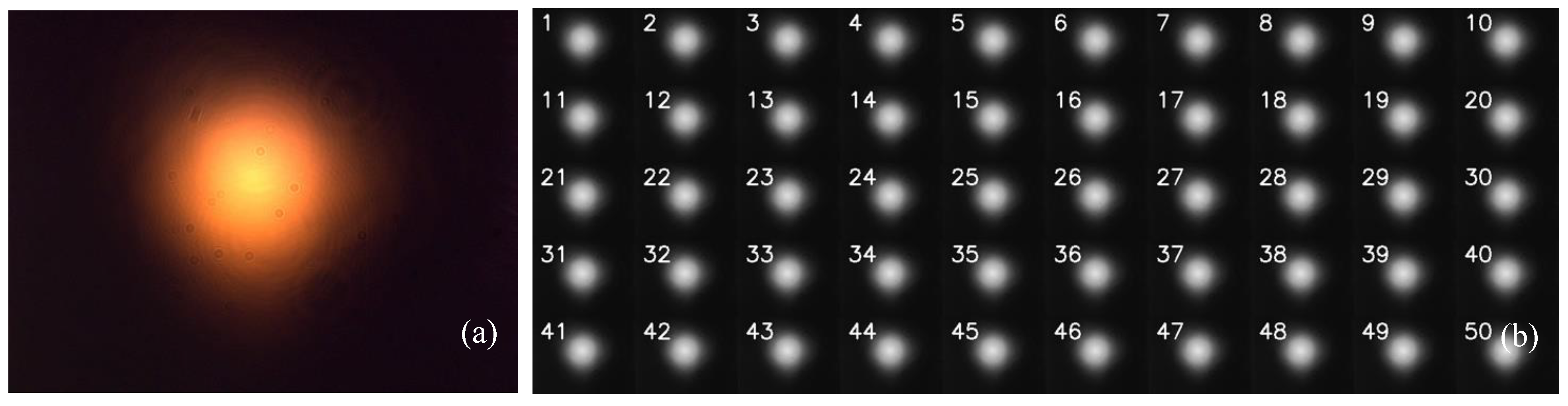
2.1. Image Data Acquisition and Preprocessing

A set of 50 beam profile images was acquired continuously under identical experimental conditions to ensure consistency and reliability in the analysis. The laser source used for this study was an Erbium-doped femtosecond fiber laser (Model EFOA-SH, Avesta, Inc., Moscow, Russia) operating at a central wavelength of 775 nm at a repetition rate of 71 MHz with a pulse duration of approximately 125 fs [16]. This ultrashort pulsed laser delivered a peak power of 13 kW and 1.2 nJ pulse energy. A neutral density (ND) filter (Model ND10A, Thorlabs, Inc., Newton, NJ, USA) was placed in the optical path to attenuate the beam intensity before it reached the camera sensor. The beam was directed onto a CCD camera (Model CS165MU, Thorlabs, Inc., Newton, NJ, USA), which is used for high-resolution image acquisition. The CCD camera provided precise spatial information about the beam, capturing intensity variations and subtle distortions. The CCD camera was connected to a computer-controlled imaging system, which captured and stored one image approximately every minute, resulting in 50 images acquired in one hour. This slow acquisition rate was intentionally chosen to allow enough time between captures for gradual thermal effects and alignment drifts to become detectable in the dataset. However, we could not acquire more than 50 images due to limitations in the laser system. Prolonged operation beyond this point led to excessive heating within the laser cavity and associated optical components, which began to degrade the beam quality. Specifically, we observed that the beam profile became increasingly distorted, with reduced spatial coherence and efficiency, making further measurements unreliable, so that the image acquisition was limited to the first hour’s stable operational window to ensure the analyzed data’s validity and consistency where the beam remained well-aligned and representative of standard system performance. The image acquisition setup is shown in Figure 1, and the optical setup was carefully aligned to minimize aberrations caused by external factors such as vibrations, air turbulence, and optical misalignments.

Each captured image underwent a structured preprocessing workflow to optimize the dataset for accurate and consistent analysis. The original beam profiles, as recorded by the CCD camera, are shown in Figure 2a. The images were first converted to grayscale to isolate the spatial intensity distribution and eliminate any potential color-channel interference, as illustrated in Figure 2b. This step ensured that only intensity values were retained for further processing. Following this, intensity normalization was applied across the dataset to correct any slight variations in exposure or laser output power, enabling a fair comparison of beam characteristics across all frames. Each grayscale image was then converted into a matrix format to prepare the beam images for numerical analysis, where each matrix element represents the intensity value of a corresponding pixel. This matrix-based representation allowed for the direct computation of key parameters such as beam centroid, FWHM, ellipticity, and asymmetry using mathematical operations on pixel data. In addition, all images were resized to a standardized resolution to ensure dimensional consistency across the dataset, which is essential for applying statistical algorithms and regression-based modeling techniques. These preprocessing steps ensured that the image dataset was uniform, comparable, and analytically robust, enabling the reliable extraction of beam properties and trend analysis across the full sequence.

2.2. Statistical and Numerical Calculations and Analysis

The numerical calculations were obtained from the preprocessed images, with the dataset consisting of matrix-form values extracted directly from the image data. Figure 3 presents a block diagram summarizing the core components of the laser beam analysis methodology. The process begins with calculations and analysis, which is the overarching approach. This then branches into two major analytical paths: beam ellipticity and width. Each of these is further examined through detailed sub-analyses; beam asymmetry stems from ellipticity, while intensity cross-section analysis builds on beam-width evaluation. This structured layout illustrates the sequential and interconnected nature of the statistical and numerical methods used in the study.

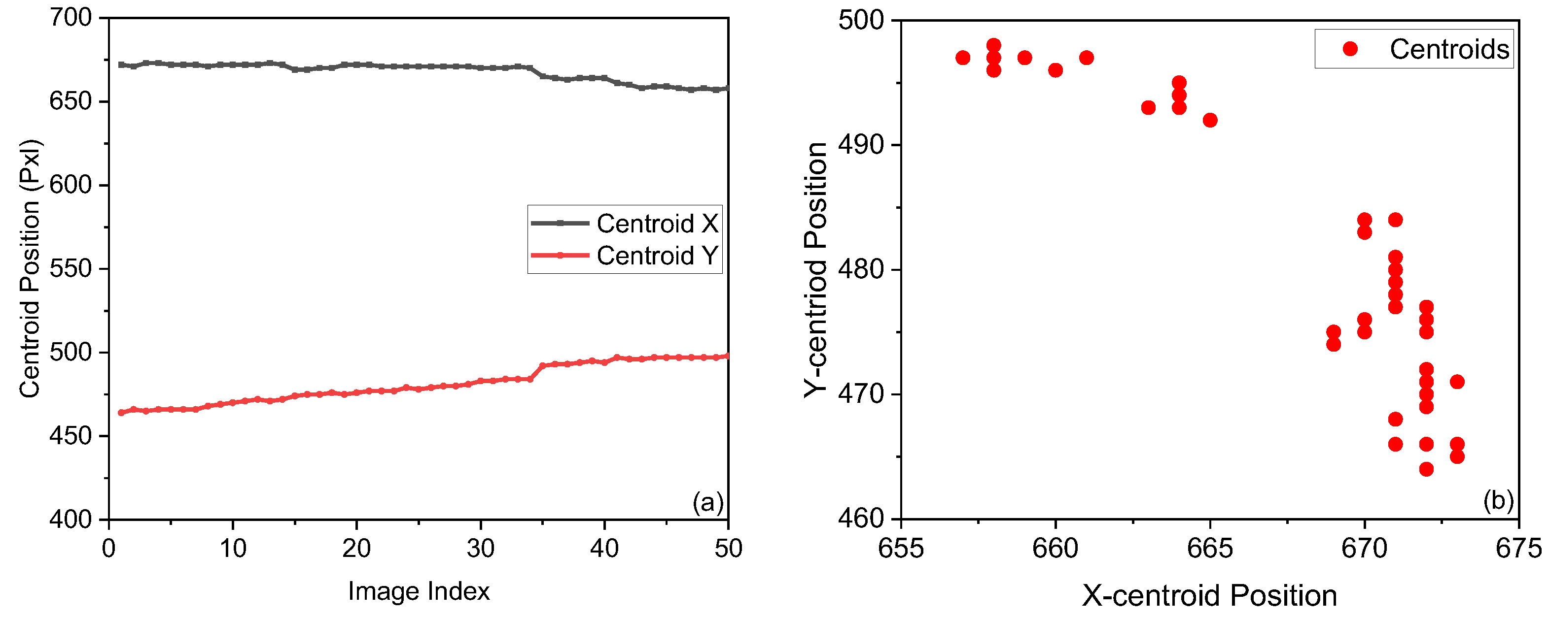
2.2.1. Beam Centroid Calculation and Analysis

The centroid of the laser beam is a crucial parameter that provides insight into the beam’s stability and spatial displacement over time. In an ideal scenario, a perfectly aligned laser beam should have a stable centroid position with minimal variations. However, external perturbations, such as thermal drift, optical misalignment, and mechanical vibrations, can cause deviations in the beam’s centroid, affecting precision applications. The centroid (X_c, Y_c) of a beam profile is computed using the weighted intensity distribution [17] across the image using Equations (1) and (2).

$${\mathrm{X}}_c={\displaystyle \frac{{\sum }_i{x}_i{I}_i}{{\sum }_i{I}_i}}$$

(1)

$${\mathrm{Y}}_c={\displaystyle \frac{{\sum }_i{y}_i{I}_i}{{\sum }_i{I}_i}}$$

(2)

I_i is the intensity at pixel (x_i, y_i), and x_i and y_i are the respective pixel coordinates. These equations ensure that the centroid calculation considers the intensity distribution, rather than just the geometric center of the image, making it a more accurate representation of the beam’s actual position.

Figure 4 shows the behavior of the centroid across the full 50-image sequence. In Figure 4a, the black curve represents the X-centroid position over time, while the red curve corresponds to the Y-centroid. It is observed that the X-centroid remains relatively stable within the range of 660 to 670 pixels throughout the sequence. However, after frame 30, a minor downward trend is noticeable, with the centroid gradually shifting from approximately 668 pixels to 664 pixels. This subtle, yet consistent, movement suggests a slow horizontal drift that could result from the thermal expansion of optical mounts or minor beam-steering instabilities. The Y-centroid shows a more prominent and progressive increase, rising from approximately 450 pixels at the start to around 500 pixels by the end of the dataset. This vertical drift is especially evident in the latter half of the acquisition period and is likely caused by systematic changes in the beam path, potentially due to temperature-induced lens deformation, beam pointing drift, or optical table settling. Figure 4b provides additional insight by plotting the X-centroid against the Y-centroid for all of the images. One cluster, located at higher X-centroid values (~668 pixels), corresponds to lower Y-centroid values (~465–480 pixels). The second cluster, at slightly lower X-centroid positions (~660–665 pixels), corresponds to higher Y-centroid values (~490–500 pixels). This inverse relationship indicates a diagonal shift in the beam position, possibly caused by a slight angular misalignment of upstream optics or thermally induced wedge effects in transmissive components. These trends highlight key insights into beam stability. The X-centroid’s downward trend and the Y-centroid’s upward trend indicate a steady shift. Monitoring centroid variations over time allows for the early detection of misalignments and facilitates corrective measures, such as the realignment of optics or compensation for systematic drifts. Even small centroid shifts of 10–20 pixels can affect optical efficiency and beam quality in precision laser applications, including beam shaping, imaging, and amplification. The combined interpretation of Figure 4 confirms that, while horizontal beam positioning is relatively stable, vertical drift increases over time, emphasizing the necessity for regular beam monitoring and adjustment strategies to maintain optimal beam alignment and high-precision performance.

2.2.2. Beam Width Estimation Using Full Width at Half Maximum (FWHM)

The laser beam width is a fundamental parameter in laser characterization, providing insights into beam divergence, focusing quality, and stability [18]. The FWHM is a widely used metric to quantify beam width, particularly for Gaussian beams. This study adopted the widely used Full Width at Half Maximum (FWHM) method to quantify beam width along the X and Y axes. FWHM is directly related to the beam’s standard deviation (σ). For an ideal Gaussian beam profile, the relationship between FWHM and σ is given by Equation (3).

$$FWHM=2\sqrt{\left(2ln2\right)}.\sigma \approx 2.355.\sigma$$

(3)

where σ is the standard deviation of the intensity profile in the respective axis (X or Y); the FWHM measurement is crucial for determining beam quality, as deviations in beam width over time or across different axes can indicate optical misalignment, thermal lensing effects, or aberrations in the laser propagation [19].

Figure 5a shows the variation of X- and Y-direction FWHM values across the entire image sequence. The red curve represents FWHM along the X-axis, while the green curve corresponds to the Y-axis. The X-FWHM starts at approximately 415 pixels and gradually increases to around 425 pixels, showing a consistent broadening trend. This behavior indicates horizontal beam divergence or degradation of collimation quality over time, potentially due to thermal-lensing effects. Meanwhile, the Y-FWHM fluctuates between 435 and 445 pixels, with an insignificant upward or downward trend. This relative stability suggests that the vertical beam profile remains more robust against temporal distortions. This lack of significant vertical divergence may be attributed to more uniform thermal dissipation or symmetric mechanical constraints in the vertical plane, which reduce the likelihood of thermal lensing effects compared to the horizontal direction. However, minor oscillations in the Y-FWHM indicate localized fluctuations, possibly caused by mechanical vibrations or minor air turbulence within the beam path. Figure 5b plots the pixel-normalized FWHM values to further validate the beam dimensions’ stability. The X-FWHM (black curve) maintains a tight band between 28 and 30 pixels, showing smaller variations than the full-frame FWHM values. The Y-FWHM (red curve) fluctuates and remains within the 38 to 40 pixels range. These patterns confirm that the horizontal beam profile is subject to a gradual divergence, whereas the vertical profile remains comparatively steady. This analysis underscores the importance of monitoring beam width over time. Changes in FWHM can significantly affect system performance, especially in tightly focused applications or when beam delivery systems rely on precise spatial confinement. The early detection of beam broadening allows for timely realignment, lens replacement, or thermal compensation to maintain optimal operation.

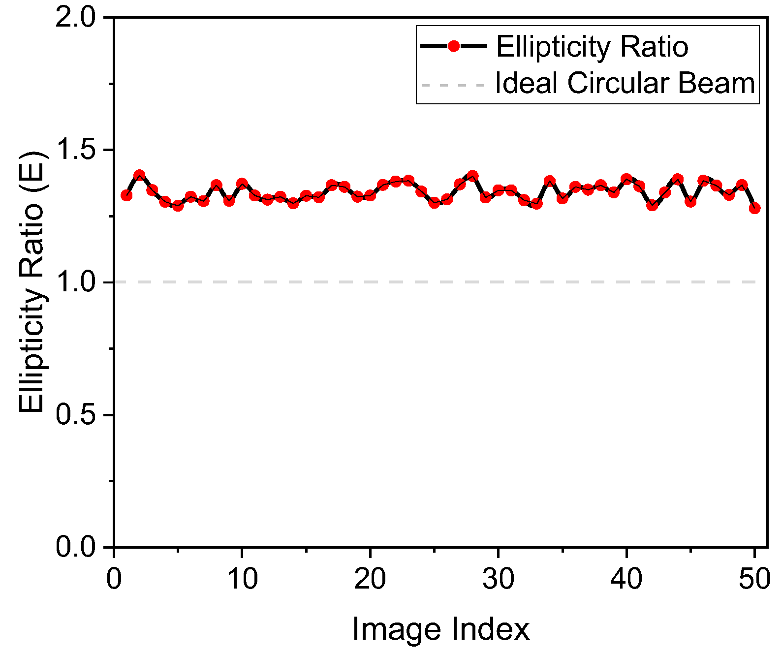
2.2.3. Beam Ellipticity Estimation Using FWHM Ratio Analysis

Beam ellipticity is a crucial metric in laser diagnostics as it offers a direct measure of the shape uniformity of the beam. While ideal laser beams are expected to exhibit a circular cross-section, especially in fundamental Gaussian modes, real-world beams often exhibit ellipticity due to slight imperfections in the optical setup, asymmetric gain profiles in the laser cavity, or differential divergence introduced by optical components such as cylindrical lenses or astigmatic beam expanders. To quantify the impact of this asymmetry, we can define an ellipticity ratio (E) as in Equation (4).

$$E={\displaystyle \frac{{FWHM}_Y}{{FWHM}_X}}$$

(4)

The plot in Figure 6 shows a beam’s ellipticity ratio (E) [20] over multiple image indices, providing insight into the beam-shape stability. The X-axis represents the image index (0 to 50), while the Y-axis represents the ellipticity ratio, ranging from ~1.3 to 1.5. The black line with red markers indicates the variation in ellipticity, while the dashed horizontal line at a ratio of 1.0 represents an ideal circular beam where the X and Y dimensions are equal. The data show that the beam consistently maintains an ellipticity ratio above 1 (E > 1), meaning the beam is elongated in one direction rather than perfectly circular. The values fluctuate slightly around 1.4, indicating small variations in beam asymmetry but no major changes in shape over time. The deviation from unity suggests that the beam’s major axis is 30% to 50% larger than the minor axis, a critical parameter in laser-beam characterization. This suggests the beam is vertically stretched, resulting in an elongated profile along the Y-axis. If a laser system requires a circular beam for optimal performance, deviations from unity indicate necessary corrections, such as beam shaping, cylindrical lens compensation, or adaptive optics. The fluctuations in the ellipticity ratio suggest possible influences from thermal effects, mechanical vibrations, or optical misalignment.

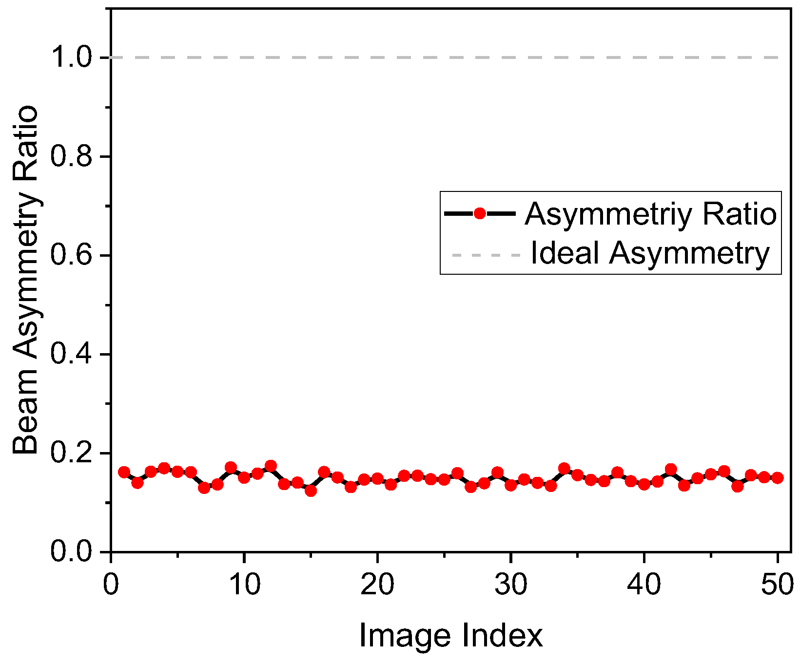
2.2.4. Beam Asymmetry Evaluation Using Directional FWHM Ratio Analysis

While ellipticity measures the proportional difference between beam dimensions, beam asymmetry offers a different lens for assessing shape uniformity, particularly the directional imbalance in beam width. Whereas ellipticity is derived from a ratio of two absolute dimensions, asymmetry focuses on the deviation from a reference of perfect symmetry, specifically, how balanced the beam is along orthogonal axes. The Symmetry Ratio (AR) of the beam is defined by Equation (5).

$$AsymmetryRatio(AR)={\displaystyle \frac{W_X}{W_Y}}$$

(5)

W_X represents the FWHM along the X-axis, and W_Y represents the FWHM along the Y-axis. A perfectly symmetric beam with AR = 1 indicates identical beam widths in both directions; deviations from this ideal value suggest stretching in either the X or Y direction.

The plot in Figure 7 illustrates the Beam Asymmetry Ratio as a function of the Image Index, covering 50 different beam profile images. The red markers connected by a line indicate the measured Asymmetry Ratio for each image, while a dashed horizontal line at y = 1.0 represents the reference for an ideally symmetric beam. The Asymmetry Ratio remains consistently below 0.2, with minor fluctuations, suggesting that the beam profiles are relatively symmetric. The values mostly range between 0.1 and 0.2, without significant deviation, indicating that the beam maintains a stable shape throughout all 50 images. However, all the Asymmetry Ratios are still below 1.0, meaning the beam is consistently stretched along the Y-axis. The fact that the Beam Asymmetry Ratio never reaches the ideal value of 1.0 confirms that the beam does not exhibit extreme asymmetry and remains well-controlled.

Minor beam asymmetries are common in practical delivery systems. Yet, they can still impact applications that demand a uniform spatial profile by introducing aberrations or reducing focus quality. The Asymmetry Ratio is a useful diagnostic tool to differentiate between shape distortion and size variation; for instance, a beam may retain stable FWHM values while shifting from a circular to an elliptical profile due to uneven stretching, which the Asymmetry Ratio reveals; however, recognizing and monitoring asymmetry remains valuable for fine-tuning the beam path in applications requiring enhanced symmetry. Beam asymmetry can be corrected using adaptive optics, real-time stabilization, optimized beam shaping, and environmental control to minimize distortions.

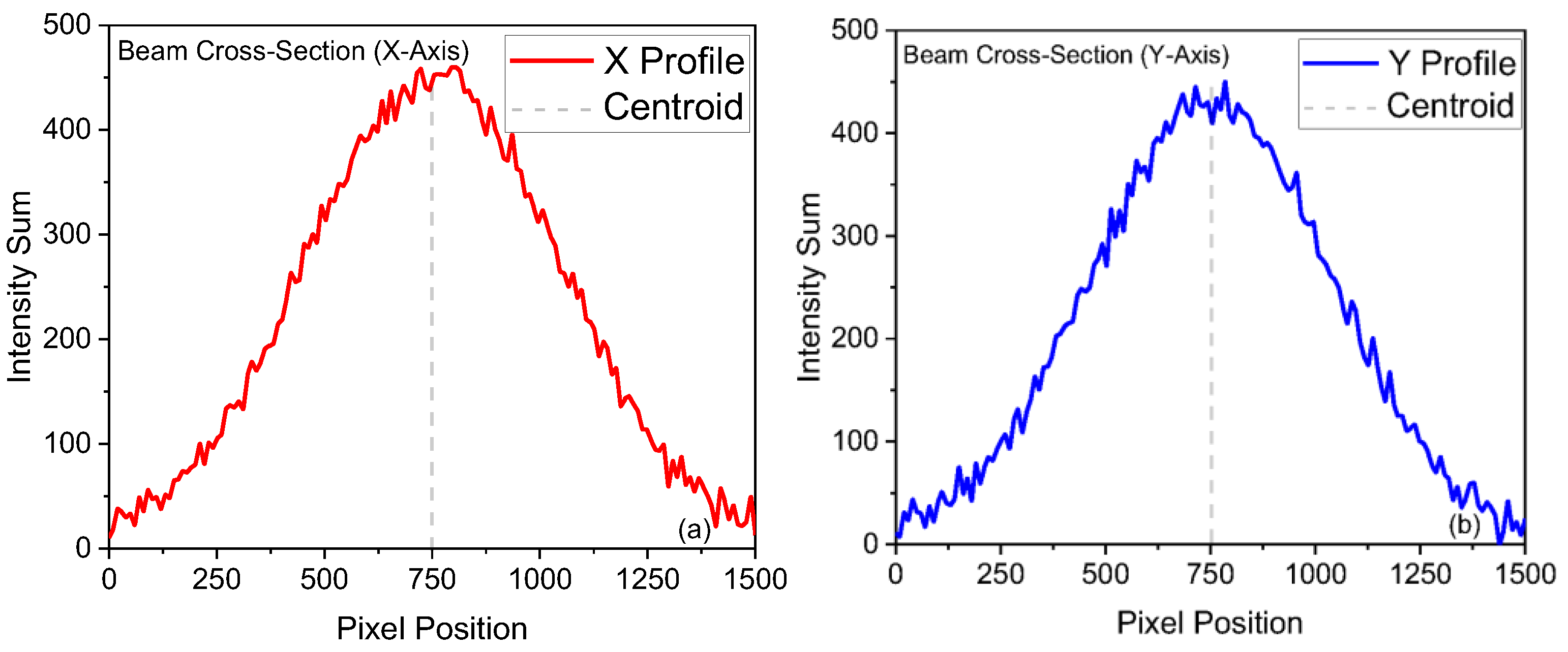
2.2.5. Intensity Cross-Sectional Analysis

To complement the centroid, width, ellipticity, and asymmetry measurements, we performed a cross-sectional intensity analysis to visualize and quantify the spatial distribution of beam intensity across the X- and Y-axes. This analysis provides a direct view of how energy is distributed within the beam and whether the profile conforms to an ideal Gaussian shape, often a desired feature in high-quality laser beams. In this method, we extracted one-dimensional intensity profiles from the two-dimensional grayscale images by integrating pixel values along each axis, yielding X-axis and Y-axis intensity profiles showing how the intensity varies horizontally and vertically, respectively. This analysis is crucial for detecting beam asymmetry, stability, and alignment issues, ensuring uniform energy distribution in laser applications [21,22].

Figure 8a displays the beam’s cross-sectional profile along the X-axis. The X-axis of the plot represents the horizontal pixel position, while the Y-axis indicates the summed intensity. A smooth, symmetric, Gaussian-like curve is observed, peaking near pixel 750, corresponding to the centroid position. The gradual and balanced tapering on either side of the peak suggests excellent beam quality in the horizontal direction, with no apparent signs of clipping or aberration. Similarly, Figure 8b shows the beam’s cross-sectional intensity along the Y-axis. The profile again appears Gaussian, with a peak intensity similar to that observed in the X-direction. The vertical line marking the centroid confirms that the beam is well-centered along both axes. No skewness, tailing, or side lobes are observed, confirming the absence of spatial mode distortion or higher-order beam artifacts.

These intensity profiles provide important cross-validation for earlier findings. The smoothness and symmetry of both profiles validate that the observed centroid drift and asymmetry are not caused by beam instabilities but rather by consistent structural differences in beam shape. Cross-sectional analysis is a valuable diagnostic tool because it provides qualitative and quantitative insights. It can reveal subtle features, such as secondary peaks, hot spots, or beam clipping, that may not be fully captured by statistical metrics alone. For instance, in industrial laser processing or laser-based surgery, non-uniform intensity distributions can cause damage, underprocessing, or uneven material interaction. Thus, routine cross-sectional analysis helps ensure quality control and application consistency.

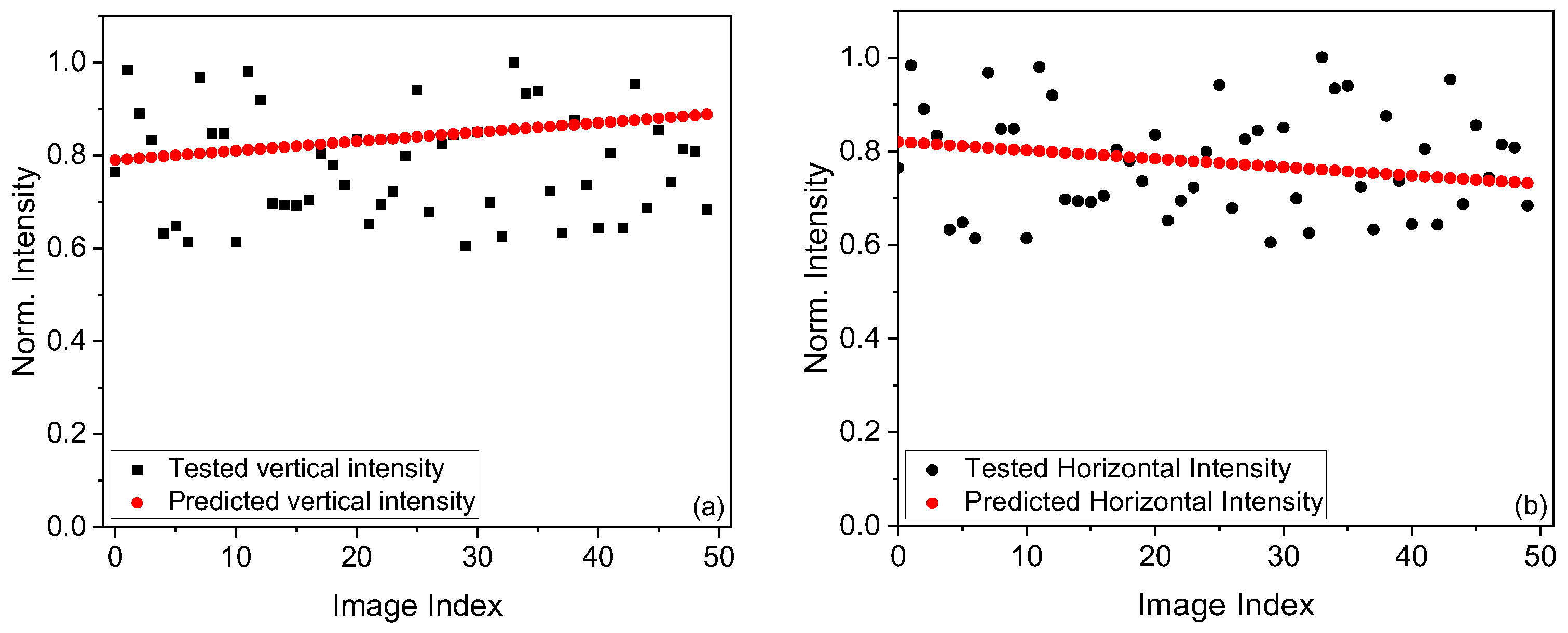
2.3. Predictive Modeling

Linear Regression

Measuring current beam characteristics and predicting future behavior is essential for maintaining long-term system performance. While traditional techniques can reveal real-time information about beam width, symmetry, or centroid position, they often fail to capture underlying trends that gradually evolve. Subtle fluctuations in beam intensity or shape caused by thermal drift, environmental changes, or optical degradation can go unnoticed in systems that rely solely on frame-by-frame analysis. Predictive modeling can be introduced as a supplementary layer of intelligence to address this limitation, capable of forecasting the beam’s dynamic behavior using statistical trends.

In this study, we used linear regression as a lightweight, supervised machine learning method, appropriate for the size and structure of our dataset. The dataset consisted of 50 beam-profile images, with extracted horizontal and vertical intensity values used as inputs. Due to the simplicity of the linear regression model and the small data volume, no complex neural network architecture or GPU-based training environment was required. The regression was implemented in a standard computing environment using basic statistical tools, which ensures reproducibility and efficiency.

Linear regression is a fundamental predictive modeling technique that establishes a relationship between a dependent and an independent variable. Regression analysis is commonly used in machine learning, where data are analyzed to find patterns and make predictions [23]. The primary goal of this regression analysis is to identify the trend in intensity variations with respect to the image index and to determine whether a consistent pattern exists. Figure 9 illustrates the step-by-step flow of the linear regression predictive modeling process used for laser-beam intensity analysis. Starting with the image index (x) and corresponding intensity values (y), the method proceeds by computing the mean values of both variables. These are then used to calculate the slope (m) and intercept (c), forming the foundation of the linear regression model. Finally, the model predicts the output intensity $\left(\overline{y}\right)$ based on the input index, enabling trend identification in laser performance.

Mathematically, the linear regression model follows Equation (6).

$$y=mx+c$$

(6)

y is the predicted intensity (either vertical or horizontal), x is the image index, m represents the slope of the regression line, and c is the intercept. To determine the best-fit line, we first computed the mean of x (image index) and y (intensity values), given by Equations (7) and (8).

$$\overline{x}={\displaystyle \frac{1}{{n\sum x}_i}}$$

(7)

$$\overline{y}={\displaystyle \frac{1}{{n\sum y}_i}}$$

(8)

where n = 50 (number of images). The slope m was calculated using Equation (9), and the intercept was determined using Equation (10).

$$m={\displaystyle \frac{\sum \left(x_i-\overline{x}\right)\left(y_i-\overline{y}\right)}{\sum {\left(x_i-\overline{x}\right)}^2}}$$

(9)

$$c=\overline{y}-m\overline{x}$$

(10)

The plots in Figure 10 were created by extracting vertical and horizontal intensity values from a sequence of laser-beam profile images, with each image assigned an index representing its order in the dataset. Each image’s vertical and horizontal intensity values were measured; these could be average or peak values across the respective axes. In the plots, the X-axis represents the image index, while the Y-axis represents the measured intensity. The black dots represent the actual measured intensity values for each image. A linear regression model was applied to the data to identify trends in intensity variation, resulting in a red line that best fits the distribution of black dots using the least squares method. This red line follows the standard linear Equation (6), and the slope is computed based on the relationship between the image indices and the corresponding intensity values. A positive slope, as seen in the vertical intensity plot in Figure 10a, indicates that intensity gradually increases with the image index, while a negative slope in the horizontal intensity plot in Figure 10b shows a declining trend. These numerically small slopes capture the directional change in intensity across the image set, and the close alignment of red and black dots confirms that the regression model accurately reflects the underlying intensity variation. Although the linear regression model exhibits some discrete scatter in Figure 10, this is primarily due to the inherent variability in the measured data points. The model was designed to capture overall trends in beam intensity rather than exact point-by-point precision. Despite the observed scatter, the fitted curves demonstrate good alignment with the general intensity variation, confirming the model’s ability to track the beam’s gradual changes over time.

From a machine-learning perspective, the intensity prediction models in the plots illustrate how linear regression, a basic supervised learning algorithm, can effectively model the relationship between image index and intensity. By minimizing the error between the measured and predicted values, the model provides a reliable fit, with residuals indicating areas for potential improvement using more advanced techniques such as polynomial regression for non-linear trends [24,25]. This approach highlights the potential of even simple machine-learning methods in laser diagnostics, offering a foundation for real-time predictive control and AI-driven optimization of laser systems.

3. Conclusions

This study demonstrates that integrating statistical analysis with machine-learning techniques can significantly enhance the accuracy and depth of laser-beam profiling. Traditional methods often rely on direct intensity measurements, which may overlook subtle but important characteristics such as beam asymmetry, centroid drift, and gradual changes in beam width (FWHM). In contrast, our approach provides a structured, data-driven way to identify and quantify these variations with greater sensitivity. The application of linear regression, a fundamental supervised machine-learning model, enabled us to detect directional trends in vertical and horizontal intensity, revealing that vertical intensity fluctuations are more pronounced. This observation may point to underlying misalignments, optical imperfections, or environmental factors affecting beam quality over time. The methodology allows us to track beam behavior across sequences of images and uncover predictive patterns that would otherwise go unnoticed. The observed trends in centroid movement and asymmetry ratios reflect the current beam quality and signal potential deviations before they escalate into major performance issues. This ability to detect early warning signs opens opportunities for developing more intelligent and responsive laser systems. By incorporating even simple machine-learning algorithms, our work highlights the practical value of AI in laser diagnostics, providing a clear pathway toward automation, adaptive correction, and real-time control in future systems. The framework established here is highly scalable and adaptable, offering the flexibility to expand into more complex models. Compared to conventional single-frame or static profiling techniques, our integrated method enhances sensitivity to subtle beam distortions and offers greater robustness by enabling temporal trend prediction through linear regression. This diagnostic framework can be applied in scenarios such as precision laser micromachining, beam alignment monitoring, and real-time stabilization systems, where consistent beam quality is essential. Nevertheless, the current study is limited by a relatively small dataset and short operational duration, which were constrained by thermal effects; future work will aim to overcome these limitations through extended acquisition and broader experimental conditions. Ultimately, this study lays a strong foundation for developing next-generation laser technologies that are more efficient, reliable, and capable of learning from their performance to self-optimize in dynamic operational environments.

References

1. Blecher, J.; Palmer, T.A.; Kelly, S.M.; Martukanitz, R.P. Identifying performance differences in transmissive and reflective laser optics using beam diagnostic tools. Weld. J. 2012, 91, 204S–214S. [Google Scholar]
2. Chouffani, K.; Harmon, F.; Wells, D.; Jones, J.; Lancaster, G. Laser-Compton scattering as a tool for electron beam diagnostics. Laser Part. Beams 2006, 24, 411–419. [Google Scholar] [CrossRef]
3. Dubey, A.K.; Yadava, V. Laser beam machining—A review. Int. J. Mach. Tools Manuf. 2008, 48, 609–628. [Google Scholar] [CrossRef]
4. Bolton, P.R.; Borghesi, M.; Brenner, C.; Carroll, D.C.; De Martinis, C.; Fiorini, F.; Flacco, A.; Floquet, V.; Fuchs, J.; Gallegos, P.; et al. Instrumentation for diagnostics and control of laser-accelerated proton (ion) beams. Phys. Medica 2014, 30, 255–270. [Google Scholar] [CrossRef]
5. Yang, G.; Liu, L.; Jiang, Z.; Guo, J.; Wang, T. The effect of beam quality factor for the laser beam propagation through turbulence. Optik 2018, 156, 148–154. [Google Scholar] [CrossRef]
6. Verhaeghe, G.; Hilton, P. The effect of spot size and laser beam quality on welding performance when using high-power continuous wave solid-state lasers. In ICALEO 2005: 24th International Congress on Laser Materials Processing and Laser Microfabrication; AIP Publishing: Melville, NY, USA, 2005. [Google Scholar]
7. Peng, W.; Jin, P.; Li, F.; Su, J.; Lu, H.; Peng, K. A review of the high-power all-solid-state single-frequency continuous-wave laser. Micromachines 2021, 12, 1426. [Google Scholar] [CrossRef] [PubMed]
8. Zhang, D.; Rolt, S.; Maropoulos, P.G. Modelling and optimization of novel laser multilateration schemes for high-precision applications. Meas. Sci. Technol. 2005, 16, 2541. [Google Scholar] [CrossRef]
9. Tan, Y.; Lin, F.; Ali, M.; Su, Z.; Wong, H. Development of a novel beam profiling prototype with laser self-mixing via the knife-edge approach. Opt. Lasers Eng. 2023, 169, 107696. [Google Scholar] [CrossRef]
10. Schäfer, B.; Lübbecke, M.; Mann, K. Hartmann-Shack wave front measurements for real time determination of laser beam propagation parameters. Rev. Sci. Instrum. 2006, 77, 053103. [Google Scholar] [CrossRef]
11. Zhang, Y.; Gao, Z.; Jin, R.; Zhao, W.; Zhu, L.; Ye, H.; Zhang, Y.; Yang, P.; Wang, S. Multi-line-of-sight Hartmann-Shack wavefront sensing based on image segmentation and K-means sorting. Opt. Express 2024, 32, 15336–15357. [Google Scholar] [CrossRef]
12. Kwee, P.; Seifert, F.; Willke, B.; Danzmann, K. Laser beam quality and pointing measurement with an optical resonator. Rev. Sci. Instrum. 2007, 78, 073103. [Google Scholar] [CrossRef]
13. Schuhmann, K.; Kirch, K.; Nez, F.; Pohl, R.; Antognini, A. Thin-disk laser scaling limit due to thermal lens induced misalignment instability. Appl. Opt. 2016, 55, 9022–9032. [Google Scholar] [CrossRef]
14. Shah, B.K.; Kedia, V.; Raut, R.; Ansari, S.; Shroff, A. Evaluation and comparative study of edge detection techniques. IOSR J. Comput. Eng. 2020, 22, 6–15. [Google Scholar]
15. Hernandez-Gonzalez, M.; Jimenez-Lizarraga, M.A. Real-time laser beam stabilization by sliding mode controllers. Int. J. Adv. Manuf. Technol. 2017, 91, 3233–3242. [Google Scholar] [CrossRef]
16. Imran, T.; Naeem, M.; Hussain, M. An experimental study of intensity-phase characterization of femtosecond laser pulses propagated through a polymethyl methacrylate. Microw. Opt. Technol. Lett. 2024, 66, e34217. [Google Scholar] [CrossRef]
17. Gu, W.; Ruan, D.; Zou, W.; Dong, L.; Sheng, K. Linear energy transfer weighted beam orientation optimization for intensity-modulated proton therapy. Med. Phys. 2021, 48, 57–70. [Google Scholar] [CrossRef] [PubMed]
18. Allegre, O.J. Laser Beam Measurement and Characterization Techniques. In Handbook of Laser Micro- and Nano-Engineering; Springer International Publishing: Cham, Switzerland, 2021; pp. 1885–1925. [Google Scholar]
19. Rondepierre, A.; Oumbarek Espinos, D.; Zhidkov, A.; Hosokai, T. Propagation and focusing dependency of a laser beam with its aberration distribution: Understanding of the halo induced disturbance. Opt. Contin. 2023, 2, 1351–1367. [Google Scholar] [CrossRef]
20. Liu, J.; Tian, X.; Chu, C.; Sui, H.; Zhang, Z.; Liang, D.; Zhang, N.; Lin, L.; Liu, W. Effect of beam ellipticity on femtosecond laser multi-filamentation regulated by π-phase plate. Laser Phys. Lett. 2020, 17, 085402. [Google Scholar] [CrossRef]
21. Wellburn, D.; Shang, S.; Wang, S.Y.; Sun, Y.Z.; Cheng, J.; Liang, J.; Liu, C.S. Variable beam intensity profile shaping for layer uniformity control in laser hardening applications. Int. J. Heat Mass Transf. 2014, 79, 189–200. [Google Scholar] [CrossRef]
22. Imran, T. Anomaly Detection in ELI-NP Front-end Laser Energy Data Using an Optimized Moving Average Method. Rom. J. Phys. 2025, 70, 902. [Google Scholar]
23. Maulud, D.; Abdulazeez, A.M. A review on linear regression comprehensive in machine learning. J. Appl. Sci. Technol. Trends 2020, 1, 140–147. [Google Scholar] [CrossRef]
24. Ostertagová, E. Modelling using polynomial regression. Procedia Eng. 2012, 48, 500–506. [Google Scholar] [CrossRef]
25. Srilakshmi, U.; Manikandan, J.; Velagapudi, T.; Abhinav, G.; Kumar, T.; Saideep, D. A new approach to computationally-successful linear and polynomial regression analytics of large data in medicine. J. Comput. Allied Intell. 2024, 2, 35–48. [Google Scholar]
Figure 1. Schematic of the experimental setup for laser beam profile analysis. The EFOA-SH Er fiber laser emits a beam directed towards a 50:50 beam splitter, which splits the beam into two paths. A mirror reflects one path while the other passes through a neutral density (ND) filter, before being captured by a CCD camera for imaging and analysis.
Photonics 12 00504 g001
Figure 2. Laser beam image dataset, (a) the actual captured image of the laser beam, (b) grayscale images derived from the original image.
Photonics 12 00504 g002
Figure 3. Block diagram illustrates the key components of beam calculations and analysis, including ellipticity, width, asymmetry, and intensity cross-section evaluation.
Photonics 12 00504 g003
Figure 4. Beam centroid position analysis: (a) centroid positions over 50 images show a stable X-centroid and the Y-centroid; (b) scatter plot of X vs. Y centroids, indicating systematic beam drift.
Photonics 12 00504 g004
Figure 5. Beam width and FWHM analysis: (a) variation of X-FWHM and Y-FWHM across the image sequence using raw pixel values; (b) corresponding normalized and smoothed values to emphasize relative trends in horizontal and vertical beam width.
Photonics 12 00504 g005
Figure 6. Ellipticity ratio variation over image indices showing a stable but non-circular beam.
Photonics 12 00504 g006
Figure 7. Beam asymmetry analysis; variation of the Asymmetry Ratio (X/Y) across 50 images.
Photonics 12 00504 g007
Figure 8. Beam cross-sectional intensity profiles: (a) along the X-axis and (b) along the Y-axis, illustrating the beam’s spatial intensity distribution. These profiles are obtained by summing intensity values across each axis, which can result in a broader visual spread than the frame-by-frame FWHM measurements shown in Figure 5.
Photonics 12 00504 g008
Figure 9. Flowchart illustrating the linear regression process for predicting laser beam intensity based on image index and intensity data.
Photonics 12 00504 g009
Figure 10. Tested value and predicted value of the normalized intensity, (a) vertical intensity shows a slightly increasing trend, (b) horizontal intensity shows a slightly decreasing trend, true values (black) are scattered, whereas predicted values (red) follow a trend.
Photonics 12 00504 g010
Disclaimer/Publisher’s Note: The statements, opinions and data contained in all publications are solely those of the individual author(s) and contributor(s) and not of MDPI and/or the editor(s). MDPI and/or the editor(s) disclaim responsibility for any injury to people or property resulting from any ideas, methods, instructions or products referred to in the content.