Experimental State Observer of the Population Inversion of a Multistable Erbium-Doped Fiber Laser

Abstract

In this work, numerical and experimental implementation of a state observer applied to an erbium-doped fiber laser (EDFL) has been developed. The state observer is designed through the mathematical model of the EDFL to estimate the non-measurable variable; however, in numerical estimation, the state variables can be measurable given the mathematical model. Only the laser intensity variable was experimentally measured. The state observer estimated the population inversion through the obtained experimental laser intensity time series fitted with their numerical laser intensity using the mean square error (MSE) tool. A bifurcation diagram of the population inversion time series local maximum was built from the state observer. The state space of the experimental laser intensity versus observed population inversion was built.

1. Introduction

The dynamics of even the simplest lasers are intimately connected to the fundamental models of nonlinear systems, linking them to a wide range of phenomena observed in various fields such as physics, engineering, and other scientific disciplines. From weather patterns to economic, chemical, and biological systems, chaotic dynamics appear to dominate [1]. Unlike these more complex systems, lasers are relatively simple, and uniquely, controlling their degrees of freedom is possible. Historically, the first experimental evidence of chaotic behavior was observed in laser physics [2], particularly in single-mode CO₂ lasers [3,4]. Studies of laser dynamics not only offer practical insights but also contribute to a broader understanding of complex yet unresolved phenomena. From the perspective of nonlinear dynamics, laser research presents clear advantages over the investigation of various physical phenomena, such as neuron dynamics [5,6,7], electronics, optoelectronics, potentially population dynamics [8,9,10], and epidemiological models [11]. Another advantage of studying lasers is that the number of degrees of freedom, such as the number of modes, can be easily controlled. In laser research, the key parameters are typically well known and controllable, and the experimental conditions are well defined.

From a theoretical perspective, studying a specific laser system involves solving differential equations analytically or, more commonly, numerically for a wide range of initial and experimental conditions. This process often generates an overwhelming amount of data, making it challenging to understand the system’s behavior fully. As a result, techniques or methods to reduce the information or the number of degrees of freedom are essential, ensuring that the core properties of dynamic evolution are retained. Experimentally, measuring or analyzing the complete temporal evolution of all the dynamic variables in a laser is typically impossible. Only partial information is recorded, which must still capture the essential dynamic characteristics of the system. In recent years, dynamic exploration of lasers has primarily focused on reduced state variables, especially optical intensity [1]. However, there has been limited attention to studying laser dynamics using the experimental state observer of the laser’s population inversion, which accounts for all state variables. Investigating the population inversion in laser models provides a way to explore chaos experimentally and draw comparisons with other well-known nonlinear systems, as discussed by Sprott [12], Rössler [13], Chen [14,15,16], Chua [17,18], and Lorenz [19]. In 1975, Haken [20] demonstrated that the Lorenz model is analogous to a laser, thereby linking their dynamics.

On the other hand, state observers are commonly employed in control systems to estimate unmeasured states based on available measurements. Various methodologies have been developed for both linear and nonlinear systems. In linear systems, least squares methods can be utilized to design observers [21]. More recent studies have concentrated on observers for uncertain nonlinear systems, employing Lyapunov stability criteria and linear matrix inequalities [22]. Critical factors in observer design include stability, convergence, and robustness against measurement noise and model uncertainties. Observers can enhance the performance of control systems by providing more precise state estimates for feedback control.

Observers have been applied across a wide range of applications, such as in walking robots [23], machine vision [24,25], power systems [26], and electric motors [27,28]. Nonlinear observer designs include Luenberger-type observers [29] and methods inspired by sliding mode control [24,25].

On the other hand, the Luenberger observer, originally designed for linear systems, has been extended to nonlinear systems in various ways. Researchers have proposed distributed Luenberger observers for networked systems [30] and developed observers for specific applications like robot manipulators [31]. Some approaches combine state and parameter estimation [32], while others focus on existence conditions and the dimensionality of Kazantzis–Kravaris/Luenberger observers [33,34]. Nonlinear extensions include the Luenberger-like observer for continuous-time systems [29] and the extended Luenberger observer for multivariable systems [35]. Numerical investigations have been conducted for infinite-dimensional vibrating systems [36]. These extensions have broadened the applicability of Luenberger-type observers to a wide range of nonlinear systems, offering improved state estimation capabilities and addressing challenges such as observability and convergence in various contexts.

For real-time control techniques, it is important to have access to all the system’s state variables (sliding modes, coupling to models, etc.) [28]. These techniques are robust in control; however, they can be applied in laser systems. Usually only the laser intensity is accessed and not the population inversion. The contribution of this research work will allow access to both state variables and make the use of control techniques easier.

This work presents the design of a Luenberger state observer for the unmeasurable variable of a multistable erbium-doped fiber laser (population inversion). The aim is to design neural identifiers and controllers that can be applied in real-time in future works.

To the best of our knowledge, this is the first time that an approximation of the variable population inversion of a laser has been experimentally demonstrated. With the contribution of this research work, we will have access to the two-state variables in addition to designing new control techniques in the laser field.

The sections of this paper are organized as follows: in Section 2, the theoretical model of the multistable erbium-doped fiber laser and normalized equations are presented; Section 3 presents the state observer design; Section 4 shows the simulation results; the experimental setup and the experimental results are given in Section 5; discussion, conclusion and some remarks about the application of state observer are drawn in Section 6.

2. Laser Model

The operation of a laser in a single emission mode is governed by three coupled equations. The key state variables are the optical field, population inversion, and polarization, each of which decays at different time scales. When one of these variables dominates, it relaxes quickly and adiabatically adjusts to the other variables, reducing the number of equations required to describe the laser.

Lasers where both population inversion and polarization decay rapidly compared to the optical field are categorized as class A lasers. In contrast, lasers where only the polarization relaxes quickly are known as class B lasers, while those where all three variables have similar relaxation rates are referred to as class C lasers. Class A lasers typically have a single constant output solution. Class B lasers exhibit energy oscillations between the optical field and population inversion, leading to relaxation oscillations. Class C lasers can display undamped periodic or non-periodic (chaotic) pulsations in their laser emissions. Furthermore, class B lasers can also exhibit periodic or chaotic dynamics if influenced externally, such as through parameter modulation. Solid-state and semiconductor lasers are examples of class B lasers. The semiconductor laser is modeled by the Lang and Kobayashi (LK) model [37]. The LK equation describes the complex dynamics of these lasers through the electric field E and population inversion (electron–hole pairs) N within the laser. Due to their rapid chaotic dynamics, these lasers have been considered for cryptographic applications in secure communication systems [38,39,40,41,42].

From a nonlinear dynamics perspective, rare-earth-doped fiber lasers with external modulation, such as solid-state, semiconductor, and gas lasers with electric discharge (e.g., ${\mathrm{CO}}_2$ and CO lasers), fall under the category of class B lasers [43]. In these systems, polarization is adiabatically eliminated, and the dynamics are described by two rate equations for the optical field and population inversion. Despite extensive research on complex laser dynamics, the nonlinear behavior of erbium-doped fiber lasers (EDFLs) has only recently been explored. The dynamic characteristics of these lasers closely resemble those of other class B lasers, with various chaotic motion scenarios being identified in EDFLs [44,45].

2.1. Complete EDFL Model

The dynamics of the EDFL studied here are modeled using two differential equations, known as power-balance equations, which incorporate excited state absorption (ESA). For erbium ions, this occurs at a wavelength of 1.5 μm. The model averages the population inversion of the EDFL and includes key factors characteristic of fiber lasers, such as ESA at the laser emission wavelength and the depletion of the pump wave as it propagates through the doped fiber. These factors lead to undamped natural oscillations in the laser, which have been experimentally observed in setups without external modulation [46,47].

The power-balance equations describe the intracavity laser emission P (defined as the sum of the intensities of the counter-propagating waves inside the cavity measured in $s^{-1}$) and the averaged population N of the upper laser level 2 (a dimensionless variable, but considering $0\le N\le 1$ ), as follows:

$$\begin{array}{cc}\hfill \dot{P}& ={\displaystyle \frac{2L}{T_r}}P\{r_w{\alpha }_0(N[\xi -\eta ]-1)-{\alpha }_{th}\}+P_{sp},\hfill \\ \hfill \dot{N}& =-{\displaystyle \frac{{\sigma }_{12}{r}_{w}P}{\pi r_0^2}}(\xi N-1)-{\displaystyle \frac{N}{\tau }}+P_{pump}.\hfill \end{array}$$

(1)

The system of Equation (1) has been widely applied in previous studies [46,48,49]. In these equations, L denotes the length of the erbium-doped fiber (EDF), and $T_r={\displaystyle \frac{2n_0(L+l_0)}{c}}$ represents the photon lifetime within the cavity, where $l_0$ is the length of the intra-cavity tails of the fiber Bragg grating (FBG) couplers. The variable P corresponds to the intracavity laser emission, with its value initially set as an initial condition.

The other parameters in Equation (1) include $r_w=1+exp\left[2{\left({\displaystyle \frac{r_0}{w_0}}\right)}^2\right]$, a factor that accounts for the match between the laser’s fundamental mode and the erbium-doped core volumes within the active fiber. Here, $r_0$ is the fiber core radius, and $w_0$ is the radius of the fundamental fiber mode. The parameter ${\alpha }_0=N_0{\sigma }_{12}$ represents the small-signal absorption of the erbium fiber at the laser emission wavelength. $N_0=N_1+N_2={2.4}^{19}{\mathrm{cm}}^{-3}$ denotes the total number of erbium ions in the active fiber, while N is defined as:

$$N={\displaystyle \frac{1}{n_{0}L}}{\int }_0^L{N}_2\left(z\right)dz,$$

where $N_2$ is the population of the upper laser level 2, and $n_0$ is the refractive index of a “cold” erbium-doped fiber core. The coefficient for the ratio between the excited-state absorption (ESA) ${\sigma }_{23}$ and the ground-state absorption cross-sections at the laser wavelength, expressed as $\xi ={\displaystyle \frac{{\sigma }_{12}+{\sigma }_{21}}{{\sigma }_{12}}}=2$ and $\eta ={\displaystyle \frac{{\sigma }_{23}}{{\sigma }_{12}}}$, considering that the cross-section of the return stimulated transition ${\sigma }_{12}$ has nearly the same intensity. The parameter ${\alpha }_{th}={\gamma }_0+{\displaystyle \frac{1}{2L}}ln\left({\displaystyle \frac{1}{R}}\right)$ represents the intra-cavity losses at the threshold, where ${\gamma }_0$ corresponds to the non-resonant fiber loss, and R defines the reflection coefficient of the FBG couplers. Additionally,

$$P_{sp}={\displaystyle \frac{{10}^{-3}N}{\tau T_r}}{\left({\displaystyle \frac{{\lambda }_g}{w_0}}\right)}^2{\displaystyle \frac{r_0^2{\alpha }_{0}L}{4{\pi }^2{\sigma }_{12}}},$$

represents the spontaneous emission into the fundamental laser mode, where $\tau$ is the lifetime of erbium ions in the excited state 2, and ${\lambda }_g$ is the laser wavelength. Finally, the pump power $P_{\mathrm{pump}}$ is defined as

$$P_{\mathrm{pump}}=P_p{\displaystyle \frac{1-exp[-\beta {\alpha }_{0}L(1-N)]}{n_0\pi r_0^{2}L}},$$

where $P_p$ denotes the pump power at the fiber input, and $\beta ={\alpha }_p/{\alpha }_0$ is the ratio of the absorption coefficients of the erbium fiber at the pump wavelength ${\lambda }_p$ and the laser wavelength ${\lambda }_g$. This study set the laser spectrum width to ${10}^{-3}$ of the erbium luminescence spectral bandwidth.

Additionally, it is important to mention that the system of Equation (1) describes the dynamics of the EDFL without considering modulation. However, a harmonic modulation of $P_p$ is introduced as

$$\begin{array}{c}\hfill P_p=P_p^0(1+m_{0}sin\left(2\pi F_{0}t\right)),\end{array}$$

(2)

where $m_0$ and $F_0$ are the modulation depth and frequency, respectively, and $P_p^0$ is the pump power without modulation at $m_0=0$.

The following parameter values, shown in Table 1 were used for the numerical implementation of the results presented in this study, consistent with those in previous works [46].

Table 1. Parameters used in numerical simulations [47,50,51,52].

Parameter	Value	Parameter	Value	Parameter	Value
L	70 cm	$n_0$	1.45	$r_0$	$1.5\times {10}^{-4}$ cm
$T_r$	8.7 nm	$l_0$	20 cm	${\omega }_0$	$3.5\times {10}^{-4}$ cm

The experimentally measured value of ${\omega }_0$ was slightly higher than $2.5\times {10}^{-4}$ cm, as predicted by the formula for a step-index single-mode fiber: $w_0=r_0(0.65+1.619/V^{1.5}+2.879/V^6)$. In this expression, the parameter V is linked to the numerical aperture $NA$ and $r_0$ by $V=2\pi r_{0}NA/{\lambda }_g$, while the values of $r_0$ and $w_0$ yield $r_w=0.308$.

The coefficients that describe the resonant absorption characteristics of the erbium-doped fiber at the emission and laser wavelengths, directly measured from a heavily doped fiber with an erbium concentration of 2300 ppm, are listed in Table 2.

Table 2. Coefficients used in numerical simulations [47,50,51,52].

Coefficient	Value	Coefficient	Value	Coefficient	Value
${\alpha }_0$	0.4 ${\mathrm{cm}}^{-1}$	$\beta$	0.5	${\sigma }_{12}$	${2.3\times 10}^{-21}$ ${\mathrm{cm}}^2$
$\xi$	2.0	$\eta$	0.4	${\sigma }_{21}$	$2.3\times {10}^{-21}{\mathrm{cm}}^2$
$\tau$	${10}^{-2}\mathrm{s}$	${\gamma }_0$	0.038	${\sigma }_{23}$	$2.3\times {10}^{-21}{\mathrm{cm}}^2$
R	0.8	${\alpha }_{th}$	$0.6\times {10}^{-21}{\mathrm{cm}}^2$	${\lambda }_g$	$1.56\times {10}^{-4}\mathrm{cm}$

By applying the specified values to the system of Equation (1), the generated wavelength ${\lambda }_g=1.56\times {10}^{-4}$ cm ($h\nu =1.274\times {10}^{-19}$ J) is experimentally observed, with the peak reflection coefficients of both FBGs aligned at this wavelength. The pump parameters are expressed in terms of the excess above the laser threshold $\epsilon$, where $P_p=\epsilon P_{th}$, and the threshold pump power is defined as follows

$$P_{th}={\displaystyle \frac{N_{th}}{\tau }}{\displaystyle \frac{n_{0}L\pi w_p^2}{1-exp\left[-{\alpha }_{0}L\beta (1-N_{th})\right]}},$$

the threshold population of level 2 is defined as

$$N_{th}={\displaystyle \frac{1}{\xi }}\left(1+{\displaystyle \frac{{\alpha }_{th}}{r_w{\alpha }_0}}\right),$$

with the pump beam radius, for simplicity, assumed to be the same as that of the generated beam (${\omega }_p={\omega }_0$).

2.2. Normalized Equations of EDFL

To synthesize and generalize the laser model, we modified the complete system (1) into the next compact expression

$$\begin{array}{c}\hfill {\displaystyle \frac{d{x}_1}{d\theta }}=x_1{x}_2-c_1{x}_1+c_2{x}_2+c_3,\end{array}$$

(3)

$$\begin{array}{c}\hfill {\displaystyle \frac{d{x}_2}{d\theta }}=-x_1{x}_2-d_1{x}_2-d_2+P_0\left(1-d_3{e}^{x_2}\right),\end{array}$$

(4)

the changes have been made in the variables:

$$\begin{array}{ccc}\hfill x_1& =& {\displaystyle \frac{{\sigma }_{12}{\Gamma }_s{T}_r{\alpha }_p}{2\pi r_0^2{\alpha }_0}}{\displaystyle \frac{{\xi }_1}{{\xi }_1-{\xi }_2}}P,\hfill \end{array}$$

(5)

$$\begin{array}{ccc}\hfill x_2& =& {\alpha }_{p}L\left(N-{\displaystyle \frac{1}{{\xi }_1}}\right),\hfill \end{array}$$

(6)

$$\begin{array}{ccc}\hfill \theta & =& {\displaystyle \frac{2r_w{\alpha }_0}{T_r{\alpha }_p}}\left({\xi }_1-{\xi }_2\right)t\hfill \end{array}$$

(7)

and in the parameters:

$$\begin{array}{ccc}\hfill c_1& =& {\displaystyle \frac{{\alpha }_{p}L}{{\xi }_1-{\xi }_2}}\left({\displaystyle \frac{{\alpha }_{th}}{{\alpha }_0{r}_w}}+{\displaystyle \frac{{\xi }_2}{{\xi }_1}}\right),\hfill \end{array}$$

(8)

$$\begin{array}{ccc}\hfill c_2& =& {\displaystyle \frac{{\xi }_1{\alpha }_p}{\pi r_w{\alpha }_0}}{\displaystyle \frac{T_r}{\tau }}{\left[{\displaystyle \frac{{\lambda }_g}{4\pi w_0\left({\xi }_1-{\xi }_2\right)}}\right]}^2\times {10}^{-3},\hfill \end{array}$$

(9)

$$\begin{array}{ccc}\hfill c_3& =& {\displaystyle \frac{L}{\pi r_w{\alpha }_0}}{\displaystyle \frac{T_r}{\tau }}{\left[{\displaystyle \frac{{\lambda }_g{\alpha }_p}{4\pi w_0\left({\xi }_1-{\xi }_2\right)}}\right]}^2\times {10}^{-3},\hfill \end{array}$$

(10)

$$\begin{array}{ccc}\hfill d_1& =& {\displaystyle \frac{{\alpha }_p}{2r_w{\alpha }_0\left({\xi }_1-{\xi }_2\right)}}{\displaystyle \frac{T_r}{\tau }},\hfill \end{array}$$

(11)

$$\begin{array}{ccc}\hfill d_2& =& {\displaystyle \frac{{\alpha }_p^{2}L}{2r_w{\alpha }_0{\xi }_1\left({\xi }_1-{\xi }_2\right)}}{\displaystyle \frac{T_r}{\tau }},\hfill \end{array}$$

(12)

$$\begin{array}{ccc}\hfill d_3& =& exp\left[-{\alpha }_{p}L\left(1-{\displaystyle \frac{1}{{\xi }_1}}\right)\right],\hfill \end{array}$$

(13)

$$\begin{array}{ccc}\hfill P_0& =& {\displaystyle \frac{{\alpha }_p^2{T}_r}{2\pi r_0^2{N}_0{r}_w{\alpha }_0\left({\xi }_1-{\xi }_2\right)}}{P}_p.\hfill \end{array}$$

(14)

The variable $x_1$ represents the normalized laser intensity, while $x_2$ corresponds to the population inversion. The parameter $P_0$ denotes the pump power, and the pump modulation, $P_p$, is given by Equation (2).

The values of the parameters used in the simulations are listed in Table 3 [53].

Table 3. Parameters for numerical simulations [47,50,51,52].

${\mathit{c}}_1$	${\mathit{c}}_2$	${\mathit{c}}_3$	${\mathit{d}}_1$	${\mathit{d}}_2$	${\mathit{d}}_3$	${\mathit{P}}_0$
$2.4$	$6.9\times {10}^{-13}$	$5.1\times {10}^{-13}$	$3.5\times {10}^{-7}$	$2.6\times {10}^{-7}$	$0.5$	$2\times {10}^{-23}{P}_p$

3. State Observer Design

Normalized equations of EDFL are given by

$$\begin{array}{cc}\hfill {\dot{x}}_1& =x_1{x}_2-c_1{x}_1+c_2{x}_2+c_3,\hfill \\ \hfill {\dot{x}}_2& =-x_1{x}_2-d_1{x}_2-d_2+u_{pump},\hfill \\ \hfill y& =x_1,\hfill \end{array}$$

(15)

where ${\dot{x}}_1$ = $d{x}_1/d\theta$, ${\dot{x}}_2$ = $d{x}_2/d\theta$ and $u_{pump}=P_0\left(1-d_3{e}^{x_2}\right)$. These equations are represented in the general form

$$\begin{array}{cc}\hfill \dot{x}& =f\left(x\right)+g\left(x\right)u_{pump},\hfill \\ \hfill y& =h\left(x\right).\hfill \end{array}$$

(16)

For system (16), the following state observer is proposed

$$\begin{array}{c}\hfill \dot{\tilde{x}}=f\left(\tilde{x}\right)+g\left(\tilde{x}\right)u_{pump}+L(y-\tilde{y}),\end{array}$$

(17)

where $\tilde{x}$ is the estimated state of $x\left(t\right)$ and $\tilde{y}\left(t\right)$ is the output from state observer, L is a constant parameter. Defining $e\left(t\right)=x\left(t\right)-\tilde{x}\left(t\right)$, the following dynamic error system results

$$\begin{array}{c}\hfill \dot{\tilde{e}}=f\left(x\right)+g\left(x\right)u_{pump}-f\left(\tilde{x}\right)-g\left(\tilde{x}\right)u_{pump}+L(y-\tilde{y}).\end{array}$$

(18)

For system (15), Equation (17) becomes

$$\begin{array}{cc}\hfill {\dot{\tilde{x}}}_1& ={\tilde{x}}_1{\tilde{x}}_2-c_1{\tilde{x}}_1+c_2{\tilde{x}}_2+c_3+L_1(x_1-{\tilde{x}}_1),\hfill \\ \hfill {\dot{x}}_2& =-{\tilde{x}}_1{\tilde{x}}_2-d_1{\tilde{x}}_2-d_2+u_{pump}+L_2(x_1-{\tilde{x}}_1),\hfill \\ \hfill \tilde{y}& ={\tilde{x}}_1.\hfill \end{array}$$

(19)

For the purpose of this work, the state observer is designed for the state variable population investment ($x_2$), given that in real time the variable cannot be measured because the electronic equipment does not exist to carry out this measurement. The stability analysis is shown in Appendix A.

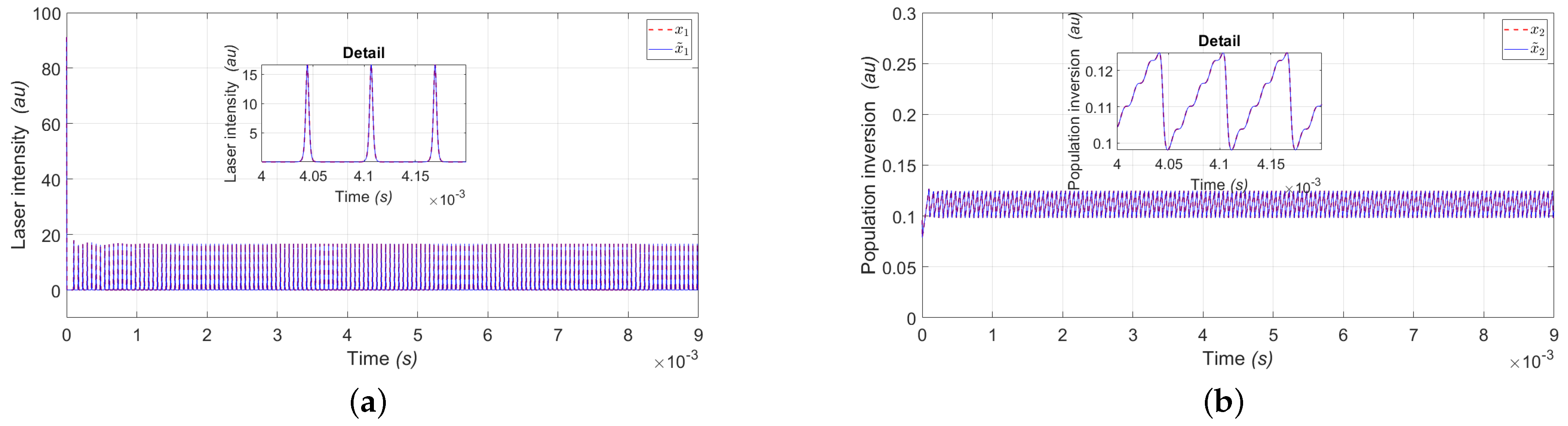
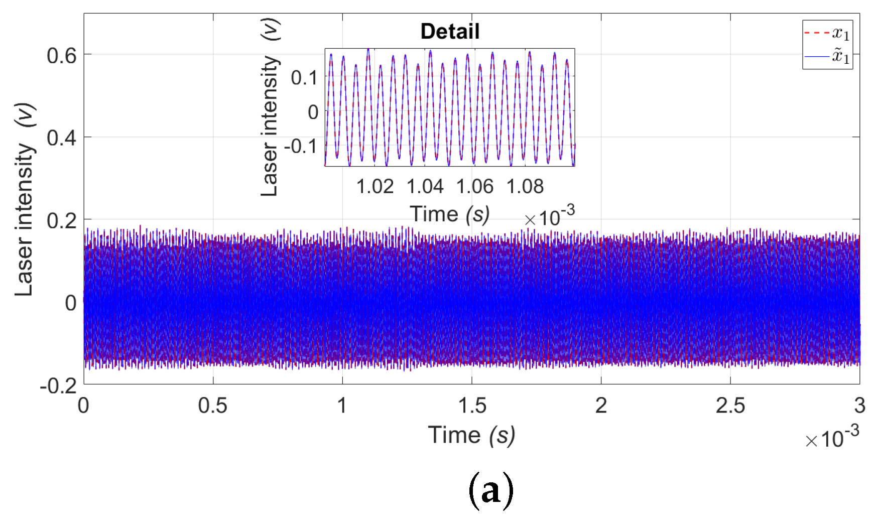
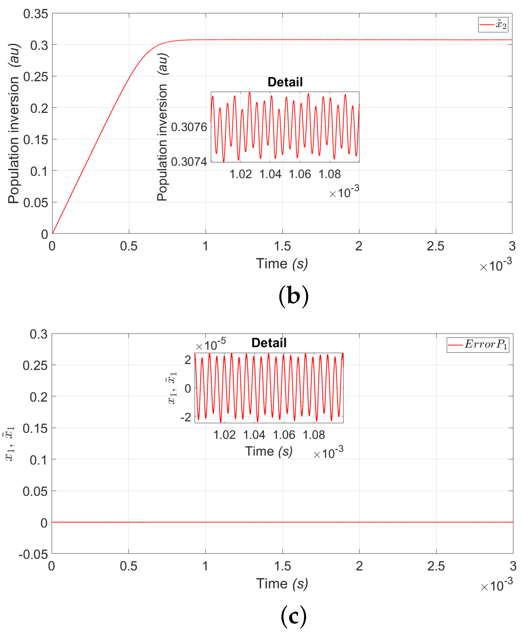
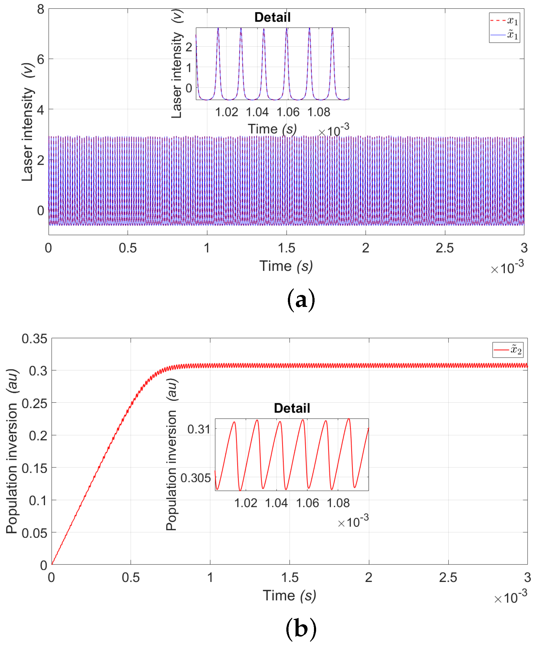
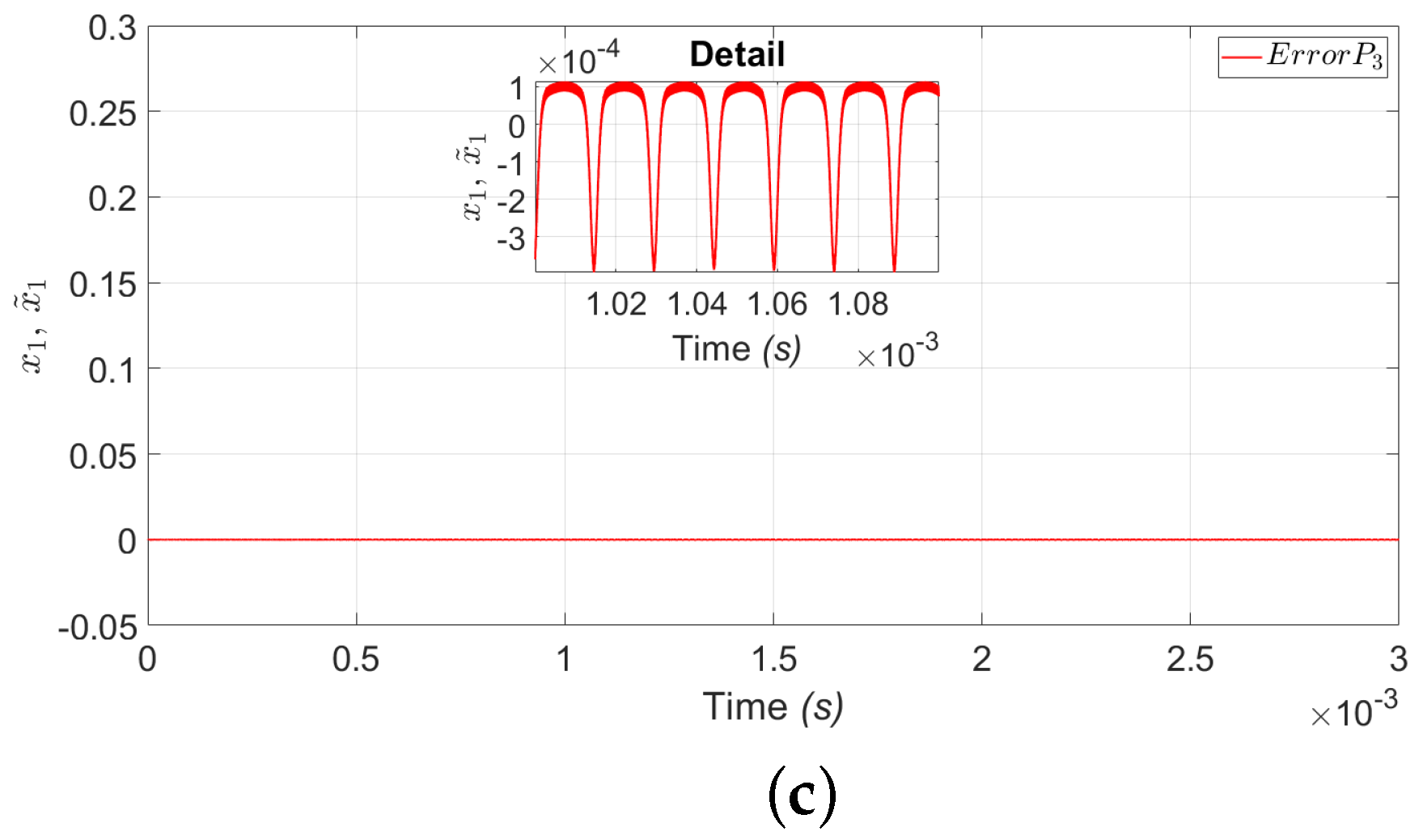
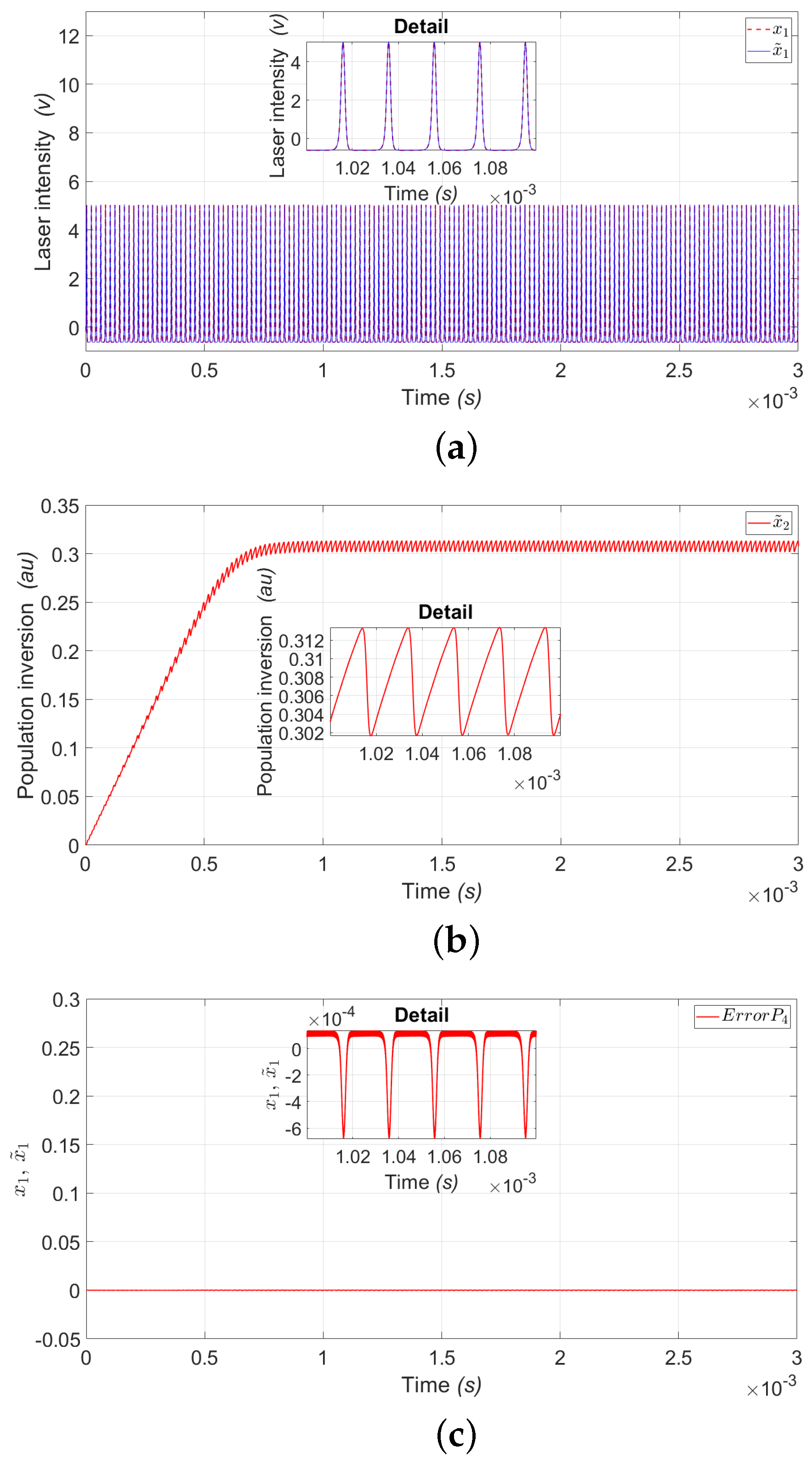
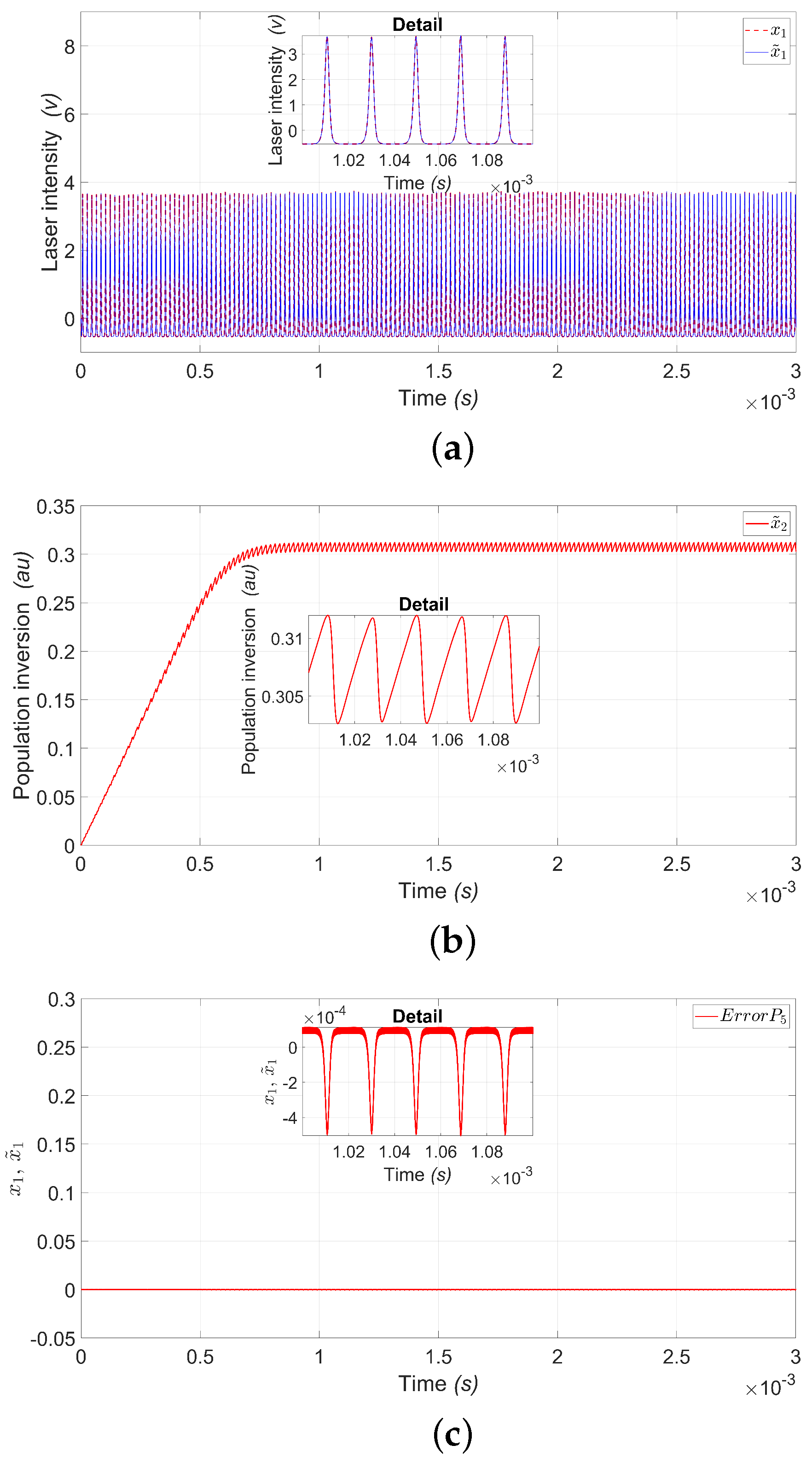
4. Simulation Results

This section shows the simulation results of the estimation of the variable of the EDFL, Equation (15) through the state observer, Equation (19), the simulation in Matlab/Simulink 2022b has been implemented.

Figure 1 shows an extract of the numerical laser intensity bifurcation diagram, which was obtained through the time series of the multistable region corresponding to the coexistence of attractors, shown by ($P1$, $P3$, $P4$, $P5$), for a modulation frequency of 80 Hz. The complete bifurcation diagram can be consulted in the work [54].

Figure 1. Bifurcation diagram for numerical laser intensity $x_1$.

The parameters used in the mathematical model of the EDFL and numerical state observer are shown in Table 3; in addition, the gains used for the state observer are $L1=0.2$ and $L2=18$.

Figure 2 shows the simulation results of the state observer for the EDFL state variables. Since the laser states in simulation can be measured, the observation of both variables for different periods is presented ($P1$, $P3$, $P4$, and $P5$). Figure 2a shows the estimation of the laser intensity ($x_1$) represented by the variable (${\tilde{x}}_1$), where we can see the convergence of the observer and Figure 2b shows the estimation of the population inversion ($x_2$) represented by the variable (${\tilde{x}}_2$); both variables are for period $P1$.

Figure 2. Simulation results of a state observer for P1: (a) laser intensity red dashed line ($x_1$) and (b) Estimated laser intensity blue continuous line (${\tilde{x}}_1$).

In the same way as Figure 2, Figure 3, Figure 4 and Figure 5 show the estimation of the laser intensity ($x_1$) represented by the variable (${\tilde{x}}_1$) and the estimate of the population inversion ($x_2$) represented by the variable (${\tilde{x}}_2$) of the periods $P3$, $P4$ and $P5$.

Figure 3. Simulation results of a state observer for P3: (a) laser intensity red dashed line ($x_1$) and (b) Estimated laser intensity blue continuous line (${\tilde{x}}_1$).

Figure 4. Simulation results of a state observer for P4: (a) laser intensity red dashed line ($x_1$) and (b) Estimated laser intensity blue continuous line (${\tilde{x}}_1$).

Figure 5. Simulation results of a state observer for P5: (a) laser intensity red dashed line ($x_1$) and (b) Estimated laser intensity blue continuous line (${\tilde{x}}_1$).

Figure 3a shows the estimation of the laser intensity ($x_1$) represented by the variable (${\tilde{x}}_1$), where we can see the convergence of the observer and Figure 3b shows the estimation of the population inversion ($x_2$) represented by the variable (${\tilde{x}}_2$); both variables are for period $P3$.

Figure 4a shows the estimation of the laser intensity ($x_1$) represented by the variable (${\tilde{x}}_1$), where we can see the convergence of the observer and Figure 4b shows the estimation of the population inversion ($x_2$) represented by the variable (${\tilde{x}}_2$); both variables are for period $P4$.

Figure 5a shows the estimation of the laser intensity ($x_1$) represented by the variable (${\tilde{x}}_1$), where we can see the convergence of the observer and Figure 5b shows the estimation of the population inversion ($x_2$) represented by the variable (${\tilde{x}}_2$); both variables are for period $P5$.

The effectiveness of the state observer depended on the correct selection of parameters and the design of the observer to ensure that the observer could provide accurate and reliable estimates. In addition, the experimental implementation of the state observer must consider aspects such as accuracy and effectiveness, as shown in the next section.

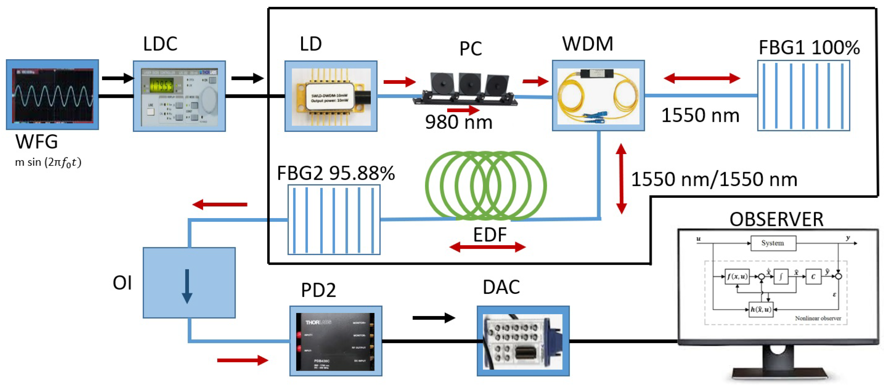
5. Experimental Setup

The implementation of the EDFL in the laboratory is shown in Figure 6. This laser has a 6.5 m resonator with a 70-centimeter erbium fiber active region, made of fiber with a core diameter of 2.7 μm, including a wavelength division multiplexing coupler (WDM-WD9850FD, Tektronix, Beaverton, OR, USA) and two fiber Bragg gratings (FBG1 and FBG2, Thorlabs, NJ, USA). The FBGs have reflectivities of 100% and 95% for use at a ${\lambda }_g=1550$ nm. The optical components are made with single-mode fiber (SMF-28, Thorlabs, New Jersey, USA) with a cladding diameter of 200 μm. The EDFL is pumped using a 977 nm laser diode (LD-BL976PAG500, Thorlabs, NJ, USA) through a polarization controller (PC) by using a laser diode controller (LDC-ITC510, Thorlabs, NJ, USA); this device also includes a temperature controlled to the pump diode. During the experiments, the diode current was set to 145.5 mA, having an EDFL threshold of 110 mA. The system was modulated with a sinusoidal signal $msin\left(2\pi f_{d}t\right)$ from a periodic function generator (WFG-AFG3102, Tektronix, Beaverton, OR, USA) applied to the pump current. An optical isolator (OI) prevents back-reflections into the laser cavities. The optical output signal $P\left(t\right)$ from the FBG2 fiber Bragg grating is directed to the PD2 photodiode, which is connected to a data acquisition card (DAC) NI-BNC-2110 for subsequent analysis. Data are collected using the DAC. Finally, the temperature of the EDFL array is always controlled.

Figure 6. Experimental setup of the EDFL. PD2 represents the photodiode, EDF is the erbium-doped fiber, FBG1 and FBG2 are fiber Bragg gratings, LDC is the laser diode controller, LD is the diode pump laser, PC is the polarization controller, WFG is the wave function generator, WDM is the wavelength-division multiplexer, OI denotes the optical isolator, and DAC refers to the data acquisition cards.

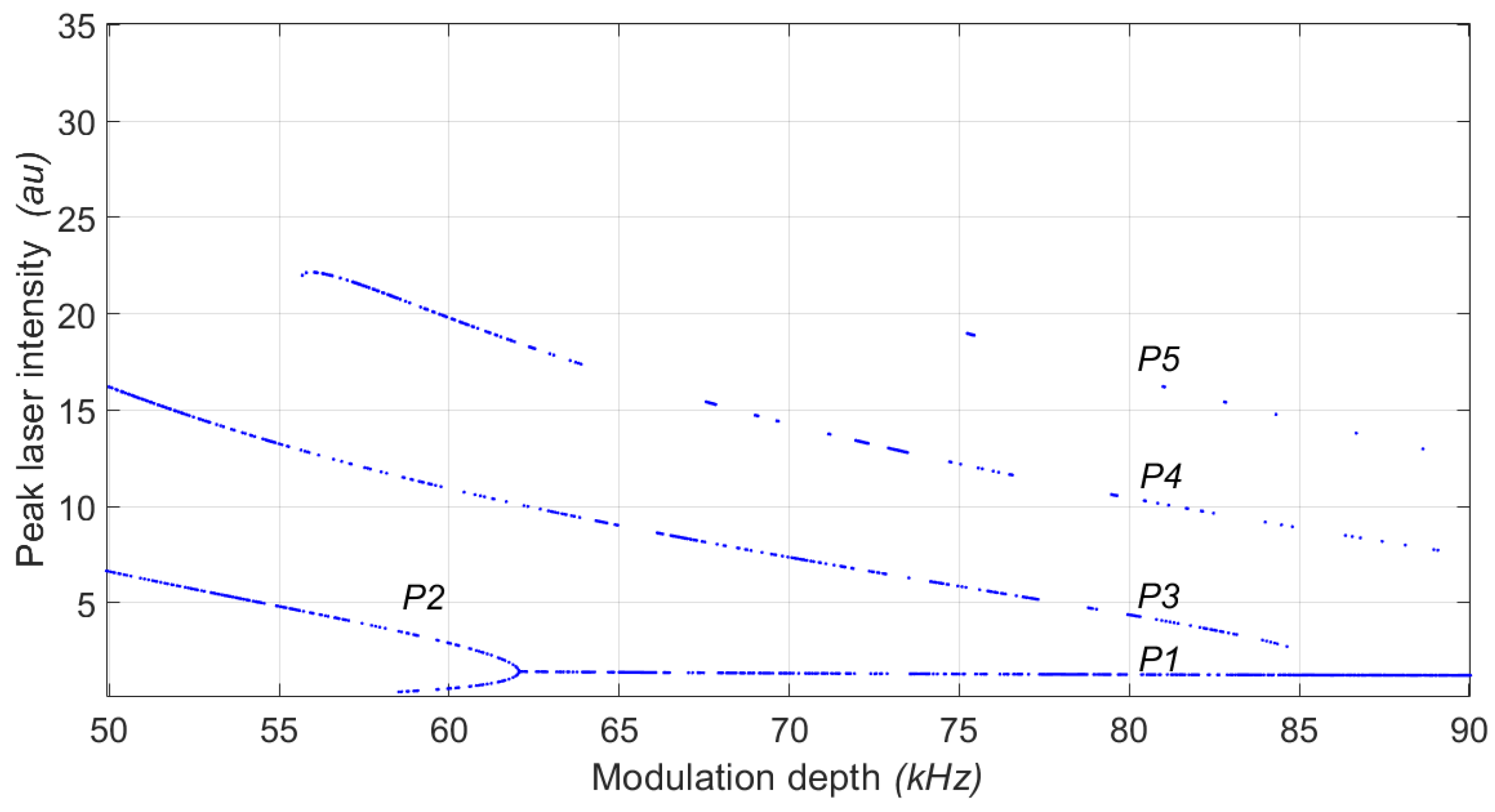
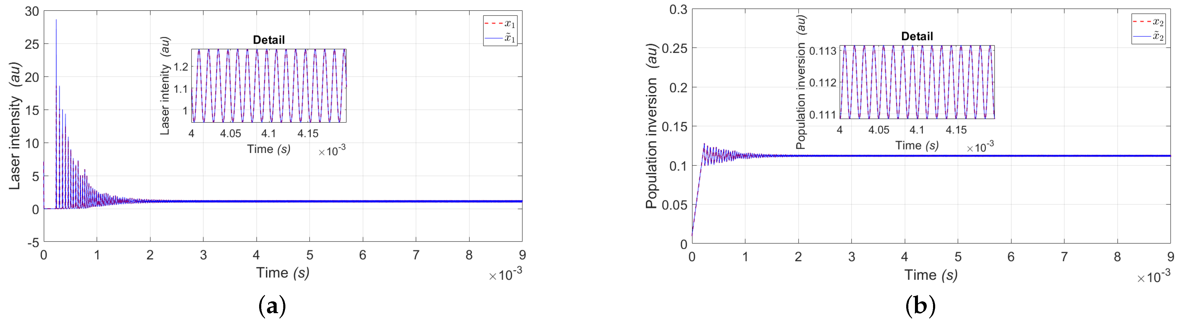
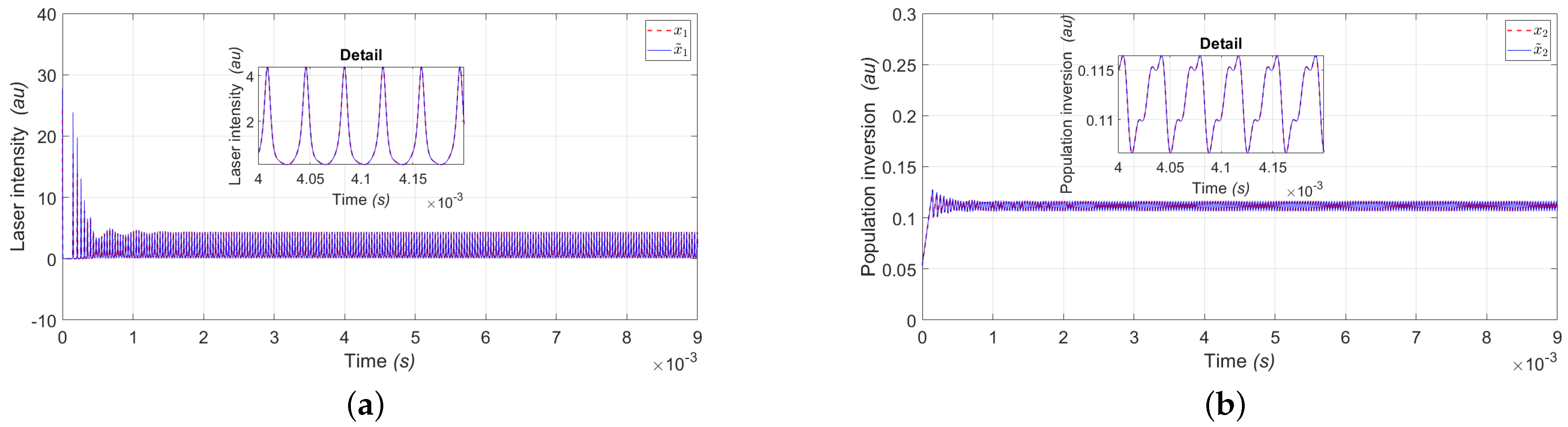
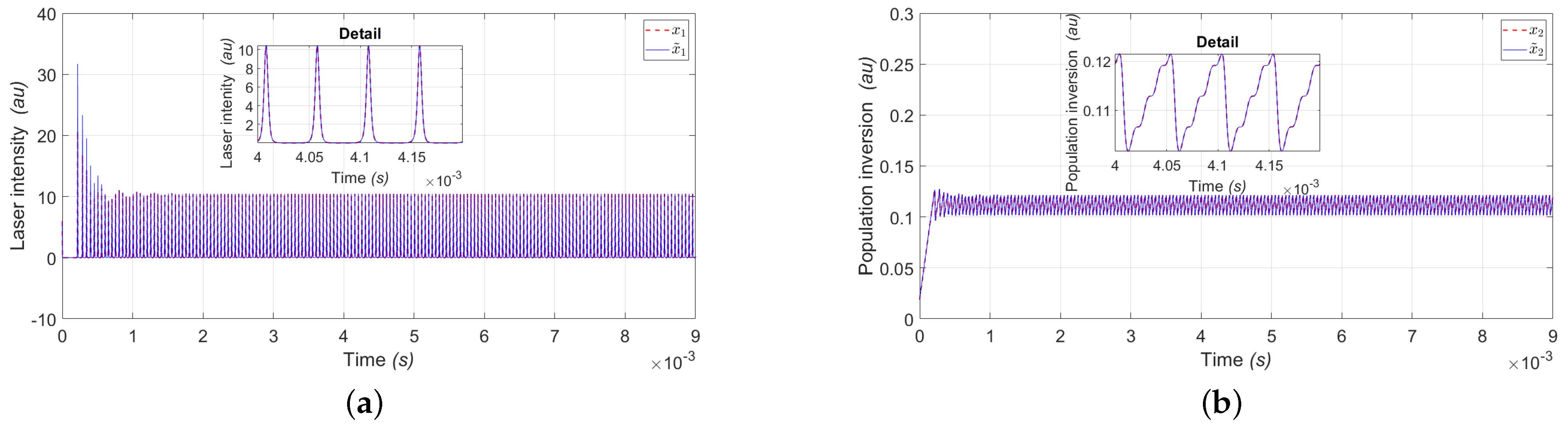
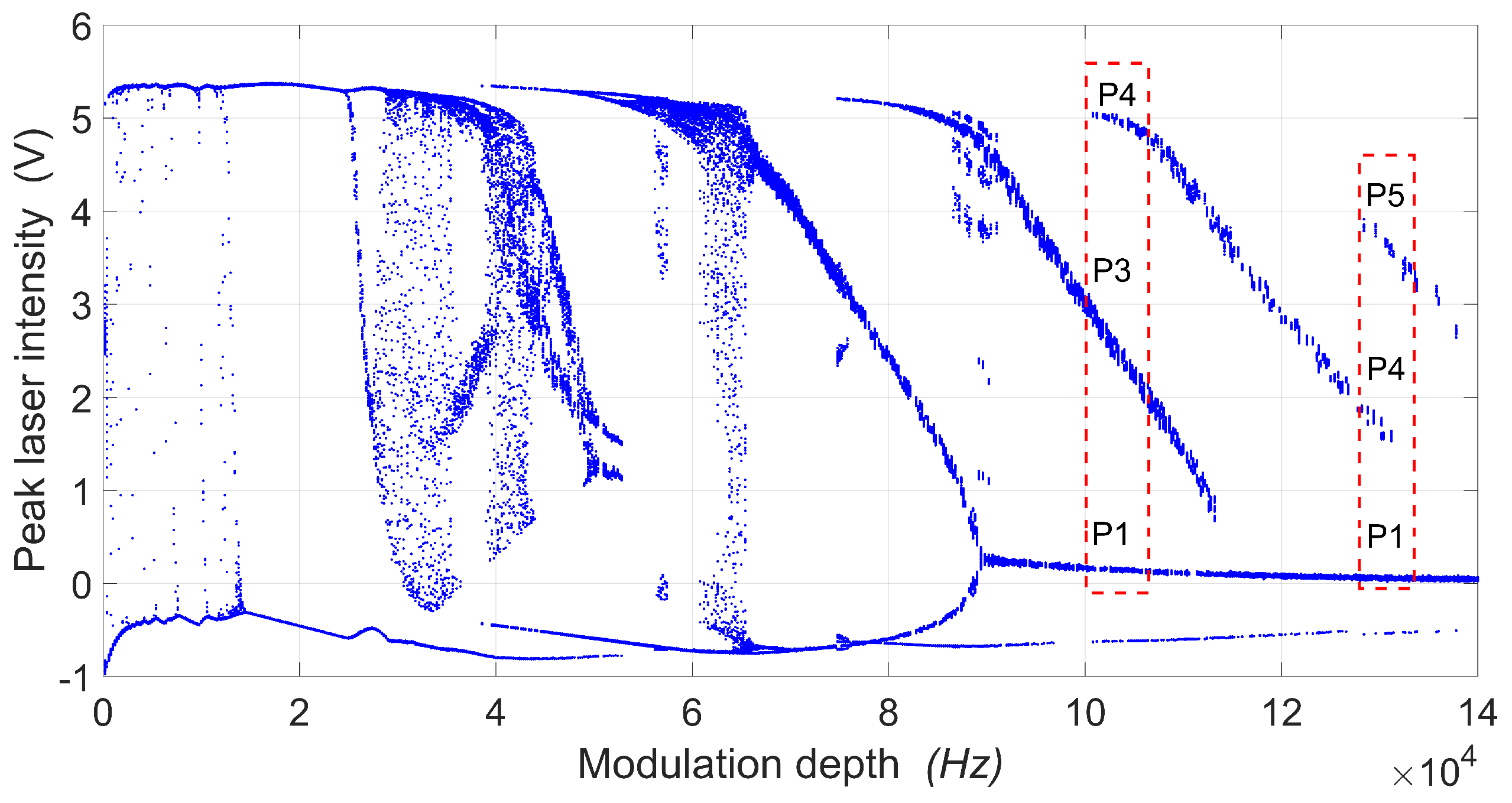
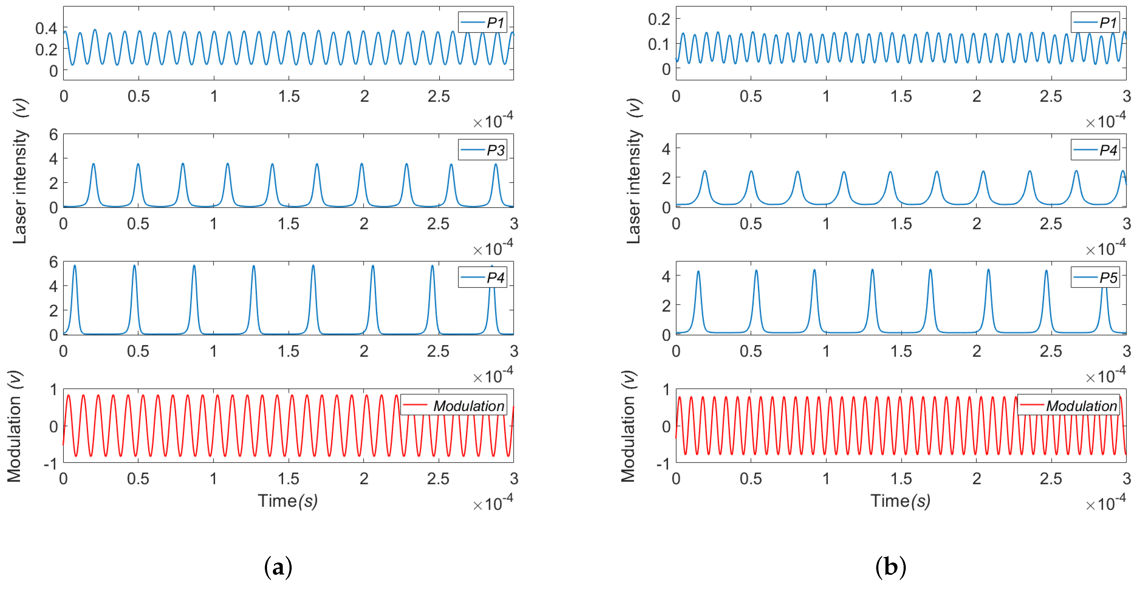
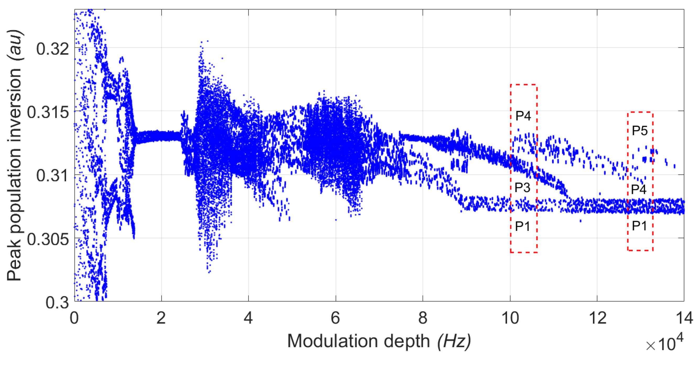
5.1. Experimental Bifurcation Diagrams and Time Series

Using periodic modulation $msin\left(2\pi f_{d}t\right)$, where m is the modulation amplitude and $f_d$ represents the frequency applied to the diode pump current via a periodic function generator (WFG), this EDFL has multistable behavior, having up to four periodic states, defined as period 1 (P1), period 3 (P3), period 4 (P4), and period 5 (P5) [46]. The output signal of the laser was detected by a photodiode (PD2) and recorded through a data acquisition card (DAC) (Figure 6). Figure 7 shows a bifurcation diagram (BD) constructed by randomly changing the system’s initial conditions by turning off and on the WFG ten times for $m=1$. The bifurcation diagram can show the system evolution corresponding to different dynamic regimes through saddle–node bifurcations when increasing the control parameter $f_d$. The attractor’s coexistence is present in different BD regions. We can see that in the range 100 kHz $<f_d<115$ kHz, P1, P3 and P4 coexist, and in the range 125 kHz $<f_d<135$ kHz, P1, P4 and P5 also coexist. The local maximum intensity in the different regimes with longer periods is significantly higher than in P1.

Figure 7. An experimental bifurcation diagram of the peak intensity of the EDFL as a function of the driving frequency $f_0$ for a fixed modulation amplitude of $m=1$ V is presented. The EDFL demonstrates the coexistence of three periodic attractors: period 1 (P1), period 3 (P3), and period 4 (P4) at a modulation frequency of $f_0=100.8$ kHz, as indicated by the red dashed line on the left side; and period 1 (P1), period 4 (P4), and period 5 (P5) at a modulation frequency of $f_0=129.6$ kHz, as shown by the red dashed line on the right side.

This section presents the experimental results for estimating the unmeasurable variables of the EDFL using the state observer Equation (19). The parameters used in the state observer Equation (19) are listed in Table 3. In addition, the gains of the experimental state observer are $L1=\mathrm{95,550.4}\times 6$ and $L2=200$. The time series of the laser intensity corresponding to different coexisting periodic regimes are shown for a modulation frequency of $f_0$ = 100,800 Hz and amplitude $m_0=1$ in Figure 8a and for a modulation frequency of $f_0$ = 129,600 Hz and amplitude $m_o=1$ in Figure 8b is shown. A modulation signal $m_{0}sin\left(2\pi f_{0}t\right)$ is shown in the bottom panel of both Figures.

Figure 8. Time series of the laser intensity of the EDFL showing the coexistence of period 1 (P1), period 3 (P3) and period 4 (P4) for (a) the modulation frequency $f_0=100.8$ kHz, as indicated by the red dashed line on the left side of Figure 7, and the coexistence of period 1 (P1), period 4 (P4) and period 5 (P5) for (b) modulation frequency $f_0=129.6$ kHz, characterized by the red dashed line on the right side of Figure 7. In both cases, the lower trace shows the modulation signal $msin\left(2\pi f_{0}t\right)$ with $m=1$ V.

Figure 9 shows the experimental results of the state observer in function of frequency for the EDFL state variables and Figure 10a shows the estimation of the laser intensity ($x_1$) represented by the variable (${\tilde{x}}_1$); although the variable can be measured physically, the procedure is carried out to guarantee good estimation of the second non-measurable variable of EDFL. Figure 10b shows the estimation of the population inversion (${\tilde{x}}_2$), and Figure 10c shows the estimation error between $x_1$ and ${\tilde{x}}_1$ where we can see that the error is very close to zero, which guarantees the good estimate of the population inversion variable.

Figure 9. Experimental bifurcation diagram for population inversion ($x_2$).

Figure 10. State observerresults for P1: (a) Experimental laser intensity red dashed line ($x_1$) and estimated laser intensity blue continuous line (${\tilde{x}}_1$). (b) Estimated population inversion red continuous line (${\tilde{x}}_2$). (c) Estimation error between ($x_1$), and (${\tilde{x}}_1$) with a modulation frequency $f_0=100.8$ kHz.

In the same way as Figure 10, Figure 11 and Figure 12 show the estimation of the laser intensity ($x_1$) represented by the variable (${\tilde{x}}_1$) and the estimate of the population inversion, represented by the variable (${\tilde{x}}_2$) of the periods $P3$, $P4$ and $P5$.

Figure 11. State observerresults for P3: (a) Experimental laser intensity red dashed line ($x_1$) and estimated laser intensity blue continuous line (${\tilde{x}}_1$). (b) Estimated population inversion red continuous line (${\tilde{x}}_2$). (c) Estimation error between ($x_1$) and (${\tilde{x}}_1$) with a modulation frequency $f_0=100.8$ kHz.

Figure 12. State observer results for P4: (a) Experimental laser intensity red dashed line ($x_1$) and estimated laser intensity blue continuous line (${\tilde{x}}_1$). (b) Estimated population inversion red continuous line (${\tilde{x}}_2$). (c) Estimation error between ($x_1$) and (${\tilde{x}}_1$) with a modulation frequency $f_0=100.8$ kHz.

Figure 11a shows the estimation of the laser intensity ($x_1$) represented by the variable (${\tilde{x}}_1$), although the variable can be measured physically. Figure 11b shows the estimation of the population inversion (${\tilde{x}}_2$), and Figure 11c shows the estimation error between $x_1$ and ${\tilde{x}}_1$ where we can see that the error is very close to zero, which guarantees the good estimate of the population inversion variable, for period $P3$.

Figure 12a shows the estimation of the laser intensity ($x_1$) represented by the variable (${\tilde{x}}_1$), although the variable can be measured physically. Figure 12b shows the estimation of the population inversion (${\tilde{x}}_2$), and Figure 12c shows the estimation error between $x_1$ and ${\tilde{x}}_1$ where we can see that the error is very close to zero, which guarantees the good estimate of the population inversion variable, for period $P4$.

Figure 13a shows the estimation of the laser intensity ($x_1$) represented by the variable (${\tilde{x}}_1$), although the variable can be measured physically. Figure 13b shows the estimation of the population inversion (${\tilde{x}}_2$), and Figure 13c shows the estimation error between $x_1$ and ${\tilde{x}}_1$ where we can see that the error is very close to zero, which guarantees the good estimate of the population inversion variable, for period $P5$.

Figure 13. State observer results for P5: (a) Experimental laser intensity red dashed line ($x_1$) and estimated laser intensity blue continuous line (${\tilde{x}}_1$). (b) Estimated population inversion red continuous line (${\tilde{x}}_2$). (c) Estimation error between ($x_1$) and (${\tilde{x}}_1$) with a modulation frequency $f_0=129.6$ kHz.

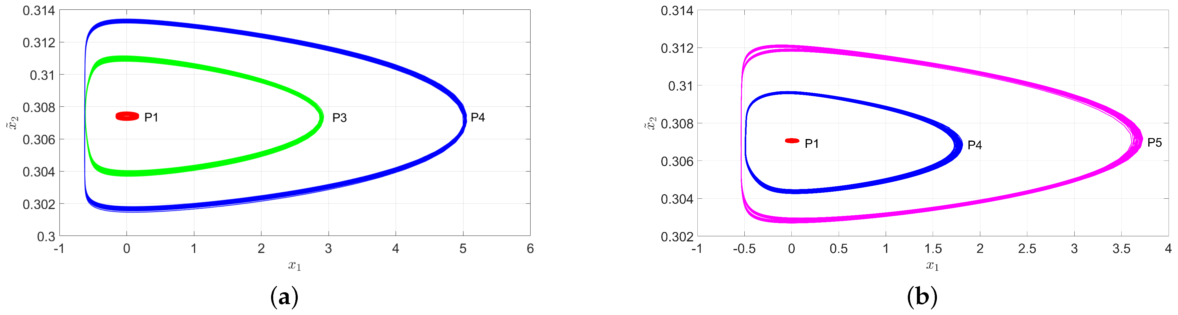
5.2. Experimental Phase Space

Figure 14a shows the phase space for periods P1, P3, and P4 of a multistable region, shown in Figure 7 with a red box at a modulation frequency of $f_0=100.8$ kHz. Similarly, for Figure 14b, the phase space of the periods P1, P4, and P5 of a multistable region is observed in Figure 7 with a red box at a modulation frequency of $f_0=129.6$ kHz. It is worth mentioning that although the periods are at different frequencies, the state observer was able to estimate each period of the multistable regions.

Figure 14. Phase space of EDFL obtained from experimental laser intensity ($x_1$) and estimated population inversion (${\tilde{x}}_2$): (a) P1, P3 and P4 with modulation $f_0$ = 100,800 Hz and (b) P1, P4 and P5 with modulation $f_0=129.6$ kHz.

5.3. Mean Square Error

The results of Table 4 show that the MSE is very small for any of the periods (P1, P3, P4 and P5), which guarantees a good estimate of the measurable laser intensity variable ($x_1$), which leads to a good estimate of the (EDFL) population inversion (${\tilde{x}}_2$).

Table 4. MSE of the state observer for laser intensity $x_1$ and estimated laser intensity ${\tilde{x}}_1$.

${\mathit{P}}_1$	${\mathit{P}}_3$	${\mathit{P}}_4$	${\mathit{P}}_5$
$0.0019$	$0.2488$	$0.0163$	$0.1303$

6. Conclusions

This paper presents the design and implementation of a nonlinear state observer to identify the non-measurable variables of an erbium-doped fiber laser (EDFL). The experimental identification of the population inversion enabled the reconstruction of the laser dynamics and the construction of a state-space model using the measurable variable (laser intensity) and the observed variable (population inversion). The mean square error (MSE) analysis confirms the accurate observation of the non-measurable variable. Furthermore, the population inversion bifurcation diagram was constructed, revealing that the multistable regions of the population inversion align with those of the laser intensity bifurcation diagram. To our knowledge, this is the first report of experimental results using a state observer for the population inversion variable in an erbium-doped fiber laser or any other type of laser. The proposed state observer technique advances the understanding of multistable dynamics in EDFLs and offers potential applications in power enhancement and intra-cavity loss control. This approach contributes significantly to the field of optics and lasers. Finally, the estimation of EDFL state variables by state observer is crucial for effectively implementing advanced controls and improving the overall performance of dynamic systems.

References

- Weiss, C.; Vilaseca, R. Dynamics of Lasers; Wiley-VCH: New York, NY, USA, 1991; Volume 1. [Google Scholar]
- Ricci, L.; Perinelli, A.; Castelluzzo, M.; Euzzor, S.; Meucci, R. Experimental Evidence of Chaos Generated by a Minimal Universal Oscillator Model. Int. J. Bifurc. Chaos 2021, 31, 2150205. [Google Scholar] [CrossRef]
- Arecchi, F.; Gadomski, W.; Meucci, R. Generation of chaotic dynamics by feedback on a laser. Phys. Rev. A 1986, 34, 1617. [Google Scholar] [CrossRef] [PubMed]
- Arecchi, F.; Meucci, R.; Gadomski, W. Laser dynamics with competing instabilities. Phys. Rev. Lett. 1987, 58, 2205. [Google Scholar] [CrossRef] [PubMed]
- Guevara, M.R.; Glass, L.; Mackey, M.C.; Shrier, A. Chaos in neurobiology. IEEE Trans. Syst. Man, Cybern. 1983, SMC-13, 790–798. [Google Scholar] [CrossRef]
- Shastri, B.J.; Nahmias, M.A.; Tait, A.N.; Wu, B.; Prucnal, P.R. SIMPEL: Circuit model for photonic spike processing laser neurons. Opt. Express 2015, 23, 8029–8044. [Google Scholar] [CrossRef]
- Tiana-Alsina, J.; Quintero-Quiroz, C.; Masoller, C. Comparing the dynamics of periodically forced lasers and neurons. New J. Phys. 2019, 21, 103039. [Google Scholar] [CrossRef]
- Volterra, V. Variazioni e Fluttuazioni del Numero D’individui in Specie Animali Conviventi; Società anonima tipografica: Pistoia, Italy, 1926. [Google Scholar]
- Lotka, A.J. Contribution to the theory of periodic reactions. J. Phys. Chem. 2002, 14, 271–274. [Google Scholar] [CrossRef]
- Lotka, A.J. Analytical note on certain rhythmic relations in organic systems. Proc. Natl. Acad. Sci. USA 1920, 6, 410–415. [Google Scholar] [CrossRef]
- Schwartz, I.B.; Smith, H. Infinite subharmonic bifurcation in an SEIR epidemic model. J. Math. Biol. 1983, 18, 233–253. [Google Scholar] [CrossRef]
- Sprott, J.C.; Sprott, J.C. Chaos and Time-Series Analysis; Oxford University Press: Oxford, UK, 2003; Volume 69. [Google Scholar]
- Rössler, O.E. An equation for continuous chaos. Phys. Lett. A 1976, 57, 397–398. [Google Scholar] [CrossRef]
- Hou, Z.; Kang, N.; Kong, X.; Chen, G.; Yan, G. On the non-equivalence of Lorenz system and Chen system. arXiv 2009, arXiv:0904.3594. [Google Scholar]
- Čelikovskỳ, S.; Chen, G. On a generalized Lorenz canonical form of chaotic systems. Int. J. Bifurc. Chaos 2002, 12, 1789–1812. [Google Scholar] [CrossRef]
- Lü, J.; Chen, G. A new chaotic attractor coined. Int. J. Bifurc. Chaos 2002, 12, 659–661. [Google Scholar] [CrossRef]
- Matsumoto, T. A chaotic attractor from Chua’s circuit. IEEE Trans. Circuits Syst. 1984, 31, 1055–1058. [Google Scholar] [CrossRef]
- Chua, L.; Komuro, M. Matsumoto: The double scroll family. IEEE Trans. Circuits Syst 1986, 33, 1072–1118. [Google Scholar] [CrossRef]
- Lorenz, E.N. Deterministic nonperiodic flow. J. Atmos. Sci. 1963, 20, 130–141. [Google Scholar] [CrossRef]
- Haken, H. Analogy between higher instabilities in fluids and lasers. Phys. Lett. A 1975, 53, 77–78. [Google Scholar] [CrossRef]
- Ling, K.; Lim, K. State observer design using deterministic least squares technique. In Proceedings of the 35th IEEE Conference on Decision and Control, Kobe, Japan, 13 December 1996. [Google Scholar]
- Farhangfar, A.; Shor, R. State Observer Design for a Class of Lipschitz Nonlinear System with Uncertainties. IFAC-PapersOnLine 2020, 53, 283–288. [Google Scholar] [CrossRef]
- Savin, S.; Jatsun, S.; Vorochaeva, L. State observer design for a walking in-pipe robot. EDP Sci. 2018, 161, 03012. [Google Scholar] [CrossRef]
- Chen, X.; Kano, H. State observer for a class of nonlinear systems and its application to machine vision. IEEE Trans. Autom. Control 2004, 49, 2085–2091. [Google Scholar] [CrossRef]
- Chen, X.; Zhai, G. State observer for a class of nonlinear systems and its application. In Proceedings of the International Conference on Control Applications, Glasgow, UK, 18–20 September 2002. [Google Scholar]
- Rosolowski, E.; Michalík, M. Fast identification of symmetrical components by use of a state observer. IEE Proc. Gener. Transm. Distrib. 1994, 141, 617–622. [Google Scholar] [CrossRef]
- Jones, L.; Lang, J. A state observer for the permanent-magnet. IEEE Trans. Ind. Electron. 1989, 36, 374–382. [Google Scholar] [CrossRef]
- Magallón, D.A.; Castañeda, C.E.; Jurado, F.; Morfin, O.A. Design of a Morlet wavelet control algorithm using super–twisting sliding modes applied to an induction machine. In Proceedings of the 2020 International Joint Conference on Neural Networks (IJCNN), Glasgow, UK, 19–24 July 2020; pp. 1–8. [Google Scholar]
- Ciccarella, G.; Dalla Mora, M.; Germani, A. A Luenberger-like observer for nonlinear systems. Int. J. Control 1993, 57, 537–556. [Google Scholar] [CrossRef]
- Kim, T.; Shim, H.; Cho, D.D. Distributed Luenberger observer design. In Proceedings of the 2016 IEEE 55th Conference on Decision and Control (CDC), Las Vegas, NV, USA, 12–14 December 2016; pp. 6928–6933. [Google Scholar]
- Celani, F. A Luenberger-style observer for robot manipulators with position measurements. In Proceedings of the 2006 14th Mediterranean Conference on Control and Automation, Ancona, Italy, 28–30 June 2006; pp. 1–6. [Google Scholar]
- Afri, C.; Andrieu, V.; Bako, L.; Dufour, P. State and parameter estimation: A nonlinear Luenberger observer approach. IEEE Trans. Autom. Control 2016, 62, 973–980. [Google Scholar] [CrossRef]
- Andrieu, V.; Praly, L. On the existence of a Kazantzis–Kravaris/Luenberger observer. SIAM J. Control Optim. 2006, 45, 432–456. [Google Scholar] [CrossRef]
- Andrieu, V.; Praly, L. Remarks on the existence of a Kazantzis-Kravaris/Luenberger observer. In Proceedings of the 2004 43rd IEEE Conference on Decision and Control (CDC)(IEEE Cat. No. 04CH37601), Nassau, Bahamas, 14–17 December 2004; Volume 4, pp. 3874–3879. [Google Scholar]
- Birk, J.; Zeitz, M. Extended Luenberger observer for non-linear multivariable systems. Int. J. Control 1988, 47, 1823–1836. [Google Scholar] [CrossRef]
- Li, X.D.; Xu, C.Z.; Peng, Y.; Tucsnak, M. On the numerical investigation of a Luenberger type observer for infinite-dimensional vibrating systems. IFAC Proc. Vol. 2008, 41, 7624–7629. [Google Scholar] [CrossRef]
- Lang, R.; Kobayashi, K. External optical feedback effects on semiconductor injection laser properties. IEEE J. Quantum Electron. 1980, 16, 347–355. [Google Scholar] [CrossRef]
- Fischer, I.; Liu, Y.; Davis, P. Synchronization of chaotic semiconductor laser dynamics on subnanosecond time scales and its potential for chaos communication. Phys. Rev. A 2000, 62, 011801. [Google Scholar] [CrossRef]
- Vanwiggeren, G.D.; Roy, R. Communication with chaotic lasers. Science 1998, 279, 1198–1200. [Google Scholar] [CrossRef]
- Donati, S.; Mirasso, C.R. Introduction to the feature section on optical chaos and applications to cryptography. IEEE J. Quantum Electron. 2002, 38, 1138–1140. [Google Scholar] [CrossRef]
- Ohtsubo, J.; Davis, P. Chaotic optical communication. Unlocking Dynamical Diversity: Optical Feedback Effects on Semiconductor Lasers; John Wiley & Sons: New York, NY, USA, 2005; pp. 307–334. [Google Scholar]
- Soriano, M.C.; Ruiz-Oliveras, F.; Colet, P.; Mirasso, C.R. Synchronization properties of coupled semiconductor lasers subject to filtered optical feedback. Phys. Rev. E 2008, 78, 046218. [Google Scholar] [CrossRef] [PubMed]
- Arecchi, F.T.; Harrison, R.G. Instabilities and Chaos in Quantum Optics; Springer Science & Business Media: Berlin/Heidelberg, Germany, 2012; Volume 34. [Google Scholar]
- Lacot, E.; Stoeckel, F.; Chenevier, M. Dynamics of an erbium-doped fiber laser. Phys. Rev. A 1994, 49, 3997. [Google Scholar] [CrossRef] [PubMed]
- Tehranchi, A.; Kashyap, R. Extremely efficient DFB lasers with flat-top intra-cavity power distribution in highly erbium-doped fibers. Sensors 2023, 23, 1398. [Google Scholar] [CrossRef] [PubMed]
- Reategui, R.; Kir’yanov, A.; Pisarchik, A.; Barmenkov, Y.O.; Il’ichev, N. Experimental study and modeling of coexisting attractors and bifurcations in an erbium-doped fiber laser with diode-pump modulation. Laser Phys. 2004, 14, 1277–1281. [Google Scholar]
- Pisarchik, A.N.; Jaimes-Reátegui, R.; Sevilla-Escoboza, R.; Huerta-Cuellar, G.; Taki, M. Rogue waves in a multistable system. Phys. Rev. Lett. 2011, 107, 274101. [Google Scholar] [CrossRef]
- Huerta-Cuellar, G.; Pisarchik, A.; Kir’yanov, A.; Barmenkov, Y.O.; del Valle Hernández, J. Prebifurcation noise amplification in a fiber laser. Phys. Rev. E 2009, 79, 036204. [Google Scholar] [CrossRef]
- Esqueda de la Torre, J.O.; García-López, J.H.; Jaimes-Reátegui, R.; Huerta-Cuellar, G.; Aboites, V.; Pisarchik, A.N. Route to chaos in a unidirectional ring of three diffusively coupled erbium-doped fiber lasers. Photonics 2023, 10, 813. [Google Scholar] [CrossRef]
- Sevilla-Escoboza, R.; Pisarchik, A.N.; Jaimes-Reátegui, R.; Huerta-Cuellar, G. Selective monostability in multi-stable systems. Proc. R. Soc. A Math. Phys. Eng. Sci. 2015, 471, 20150005. [Google Scholar] [CrossRef]
- Pisarchik, A.; Jaimes-Reátegui, R.; Sevilla-Escoboza, R.; Huerta-Cuellar, G. Multistate intermittency and extreme pulses in a fiber laser. Phys. Rev. E Statistical, Nonlinear, Soft Matter Phys. 2012, 86, 056219. [Google Scholar] [CrossRef]
- Huerta-Cuellar, G.; Pisarchik, A.N.; Barmenkov, Y.O. Experimental characterization of hopping dynamics in a multistable fiber laser. Phys. Rev. E Statistical, Nonlinear, Soft Matter Phys. 2008, 78, 035202. [Google Scholar] [CrossRef] [PubMed]
- Pisarchik, A.N.; Kir’yanov, A.V.; Barmenkov, Y.O.; Jaimes-Reátegui, R. Dynamics of an erbium-doped fiber laser with pump modulation: Theory and experiment. J. Opt. Soc. Am. B 2005, 22, 2107–2114. [Google Scholar] [CrossRef]
- Magallón, D.A.; Jaimes-Reátegui, R.; García-López, J.H.; Huerta-Cuellar, G.; López-Mancilla, D.; Pisarchik, A.N. Control of multistability in an erbium-doped fiber laser by an artificial neural network: A numerical approach. Mathematics 2022, 10, 3140. [Google Scholar] [CrossRef]
Disclaimer/Publisher’s Note: The statements, opinions and data contained in all publications are solely those of the individual author(s) and contributor(s) and not of MDPI and/or the editor(s). MDPI and/or the editor(s) disclaim responsibility for any injury to people or property resulting from any ideas, methods, instructions or products referred to in the content. |
© 2024 by the authors. Licensee MDPI, Basel, Switzerland. This article is an open access article distributed under the terms and conditions of the Creative Commons Attribution (CC BY) license (https://creativecommons.org/licenses/by/4.0/).