Station Arrangement Optimization of Photoelectric Theodolites Based on Efficient Traversing Discrete Points

Abstract
1. Introduction
2. Optimization Model of Station Arrangement
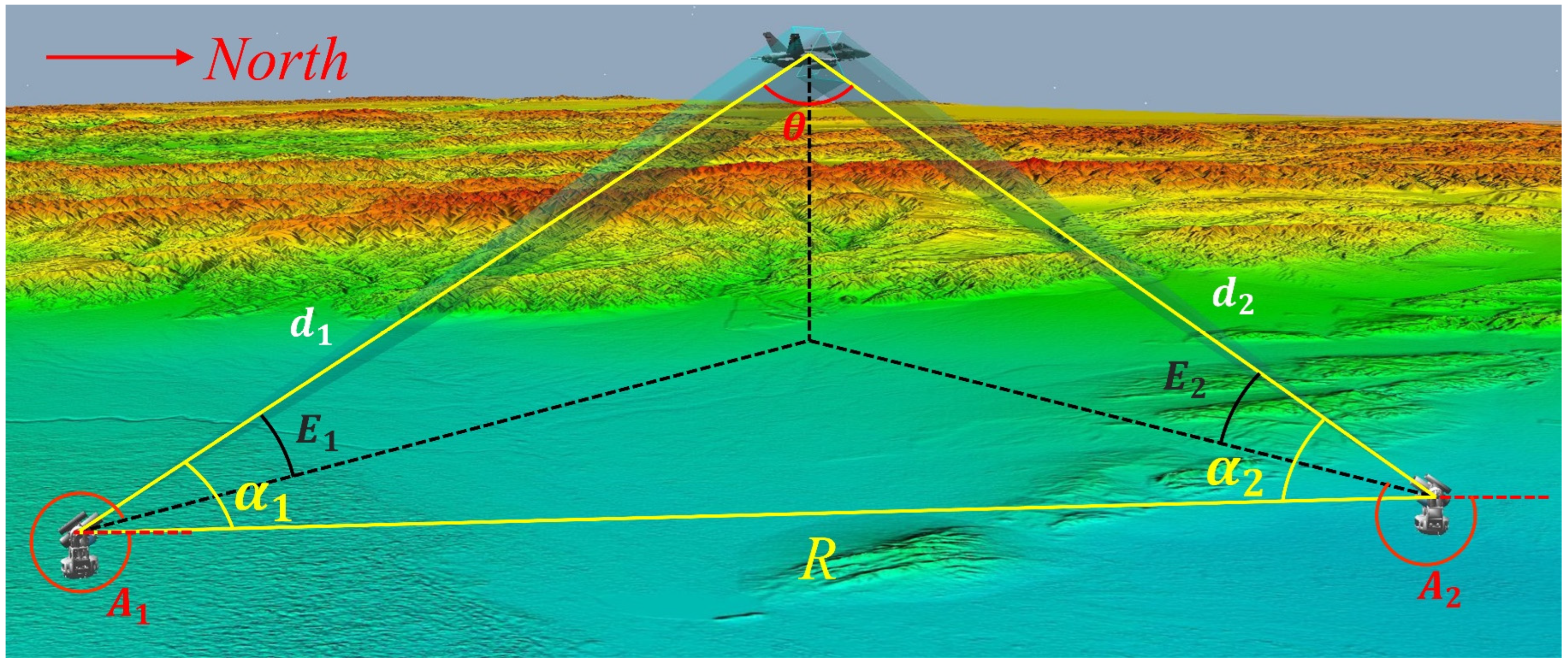
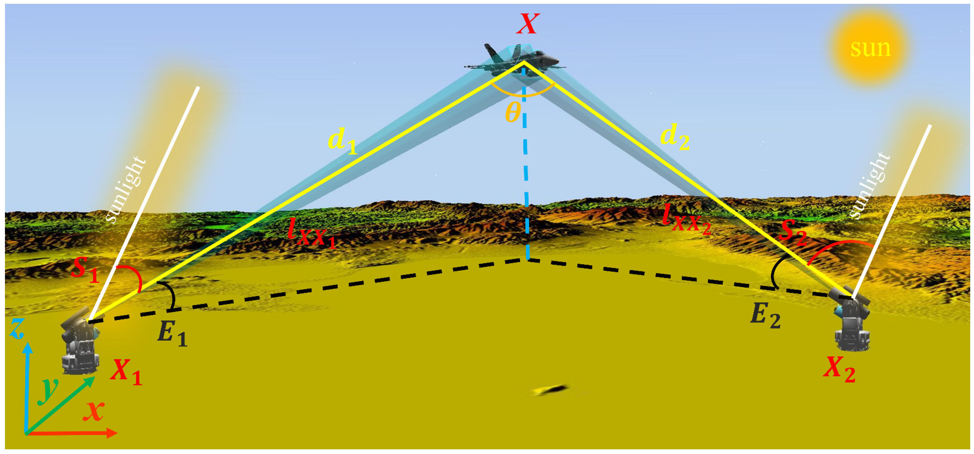
2.1. Principle of Intersection Measurement
2.2. Objective Function
2.3. Constraint Conditions
3. Discretization of Optimization Model
3.1. Discretize Optimization Model
3.2. Solution to Terrain Obstruction
4. The Fast Traversal Algorithm
4.1. Acceleration Strategy
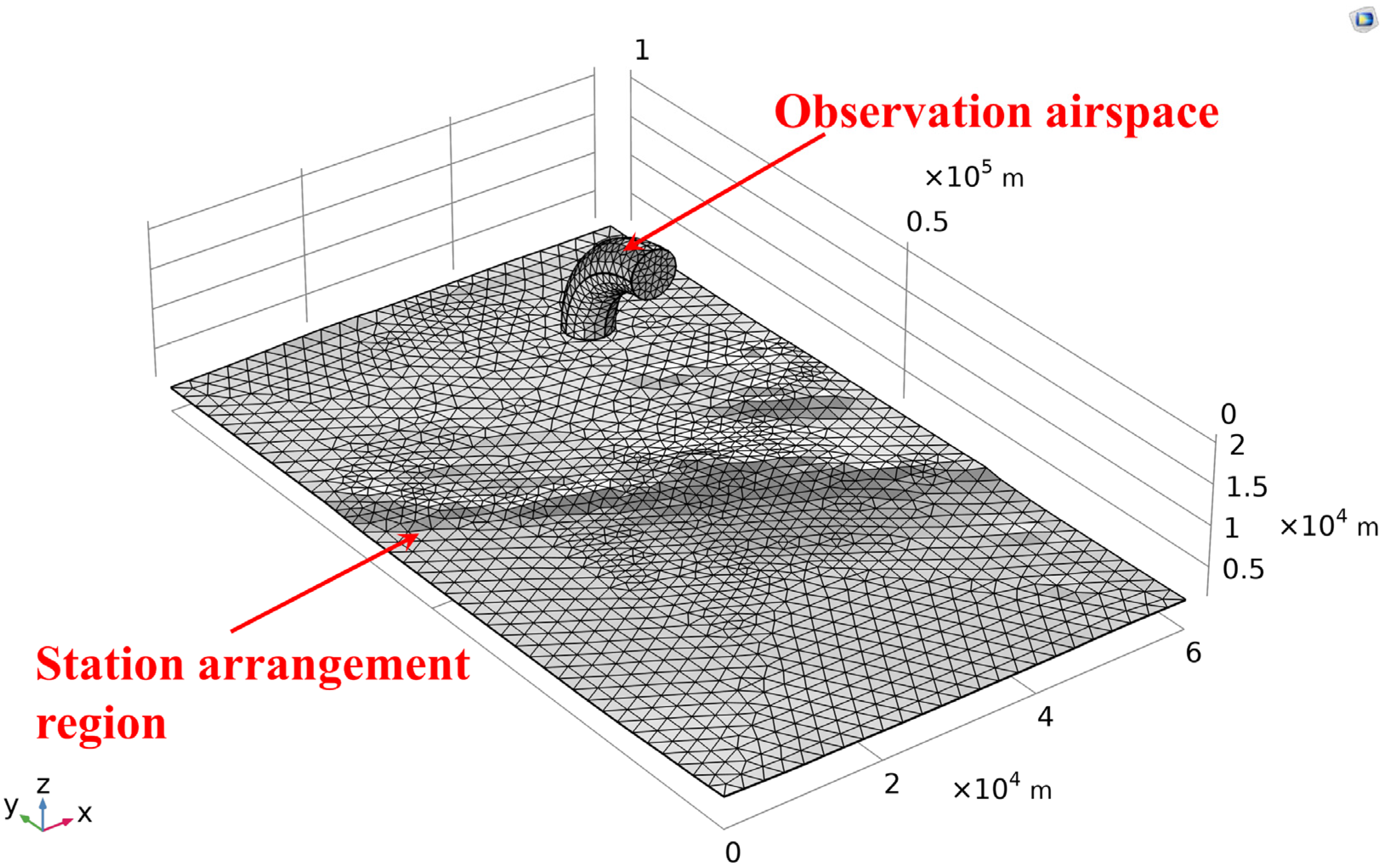
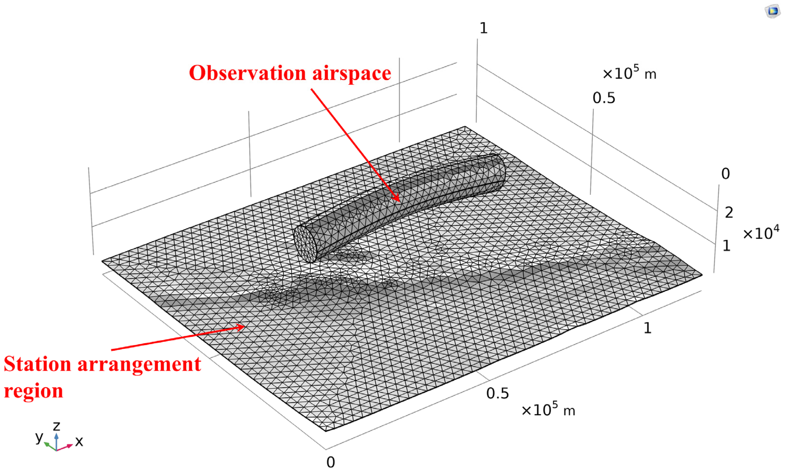
4.1.1. Reducing the Discrete Dimension of the Airspace
4.1.2. Solving Intersection Angle with Euclidean Distance Matrix
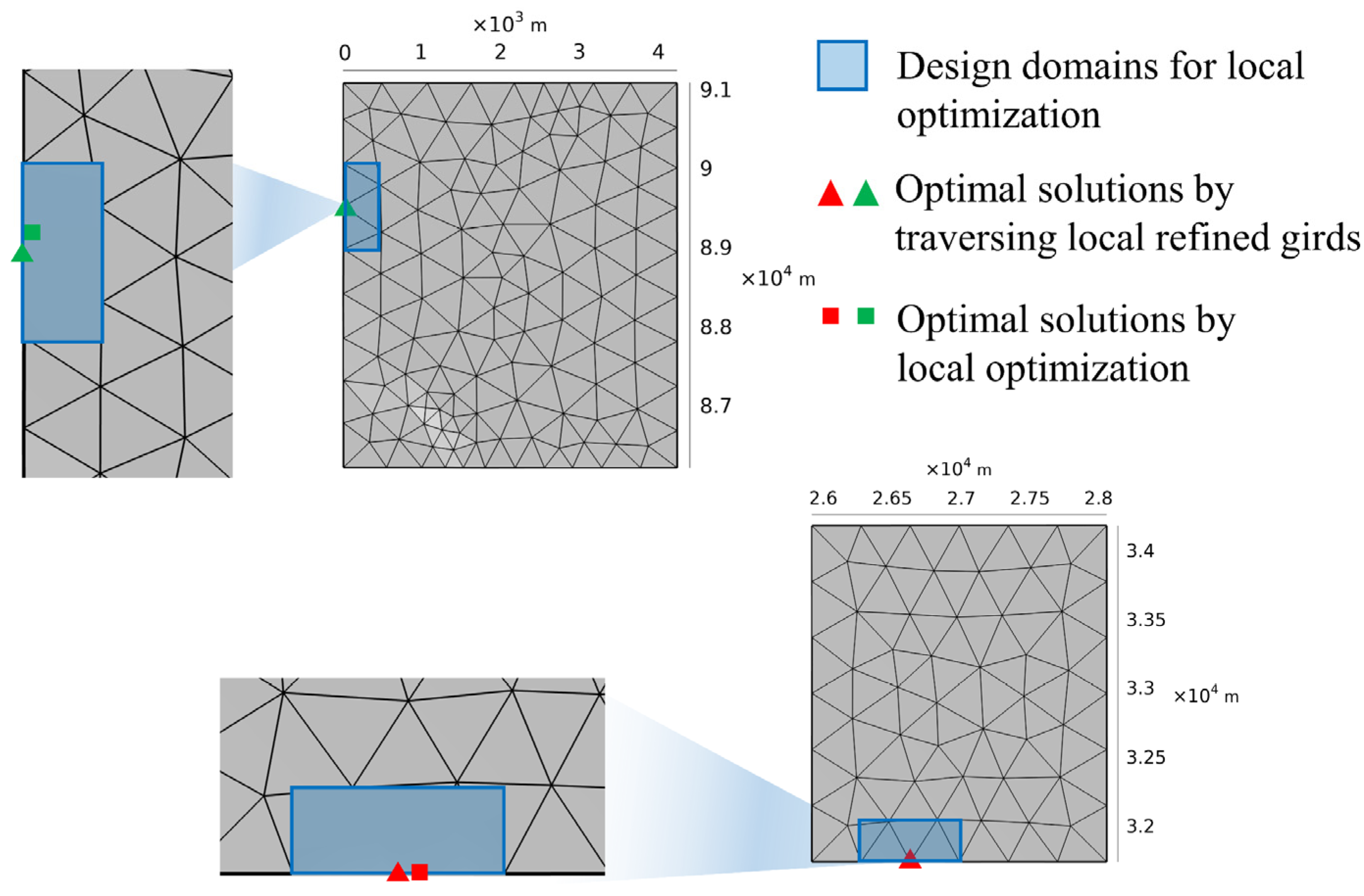
4.2. Improve Precision of Station Arrangement via Local Optimization
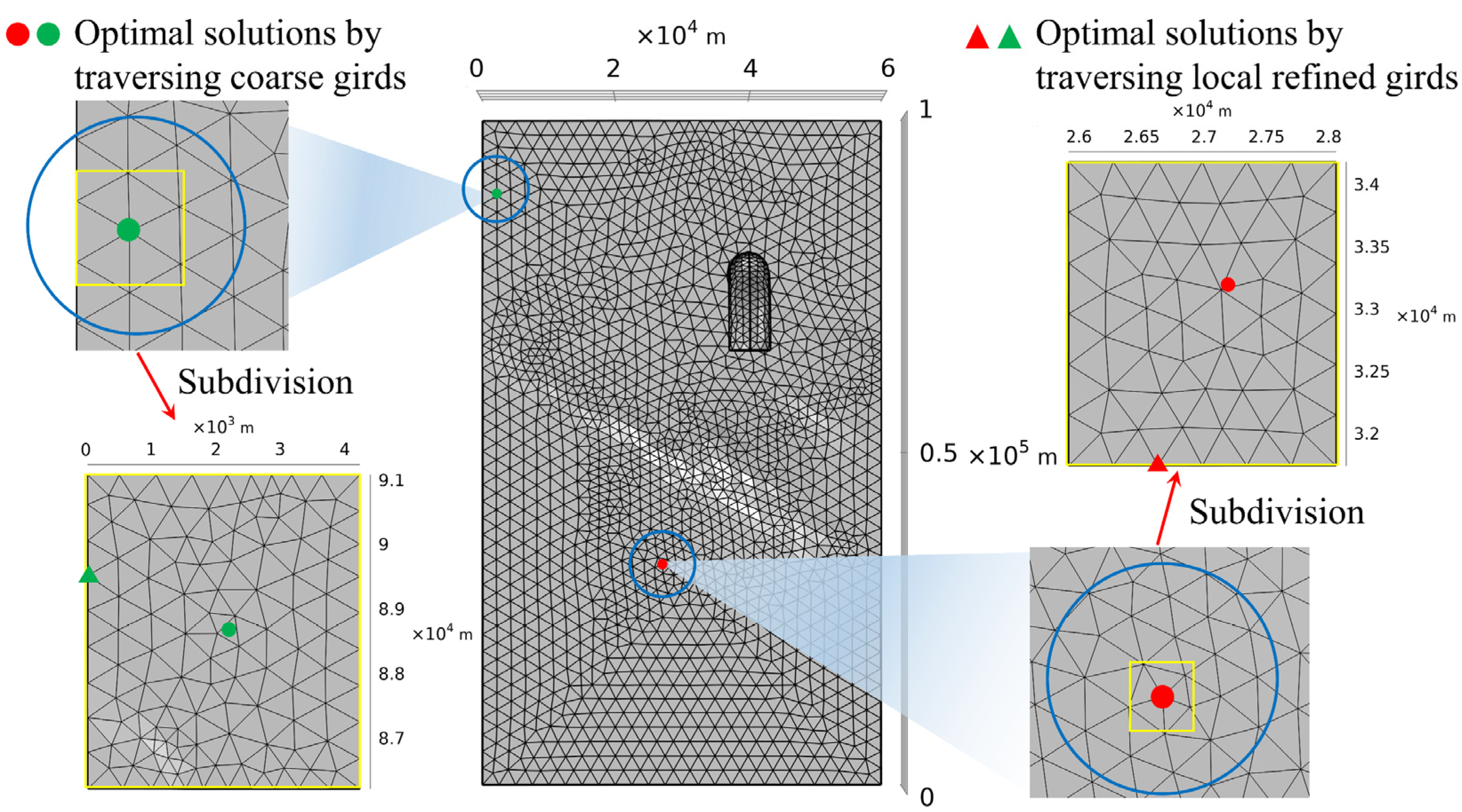
4.2.1. Local Grid Refinement
4.2.2. Solving by Fitting Continuous Terrain
5. Numerical Examples
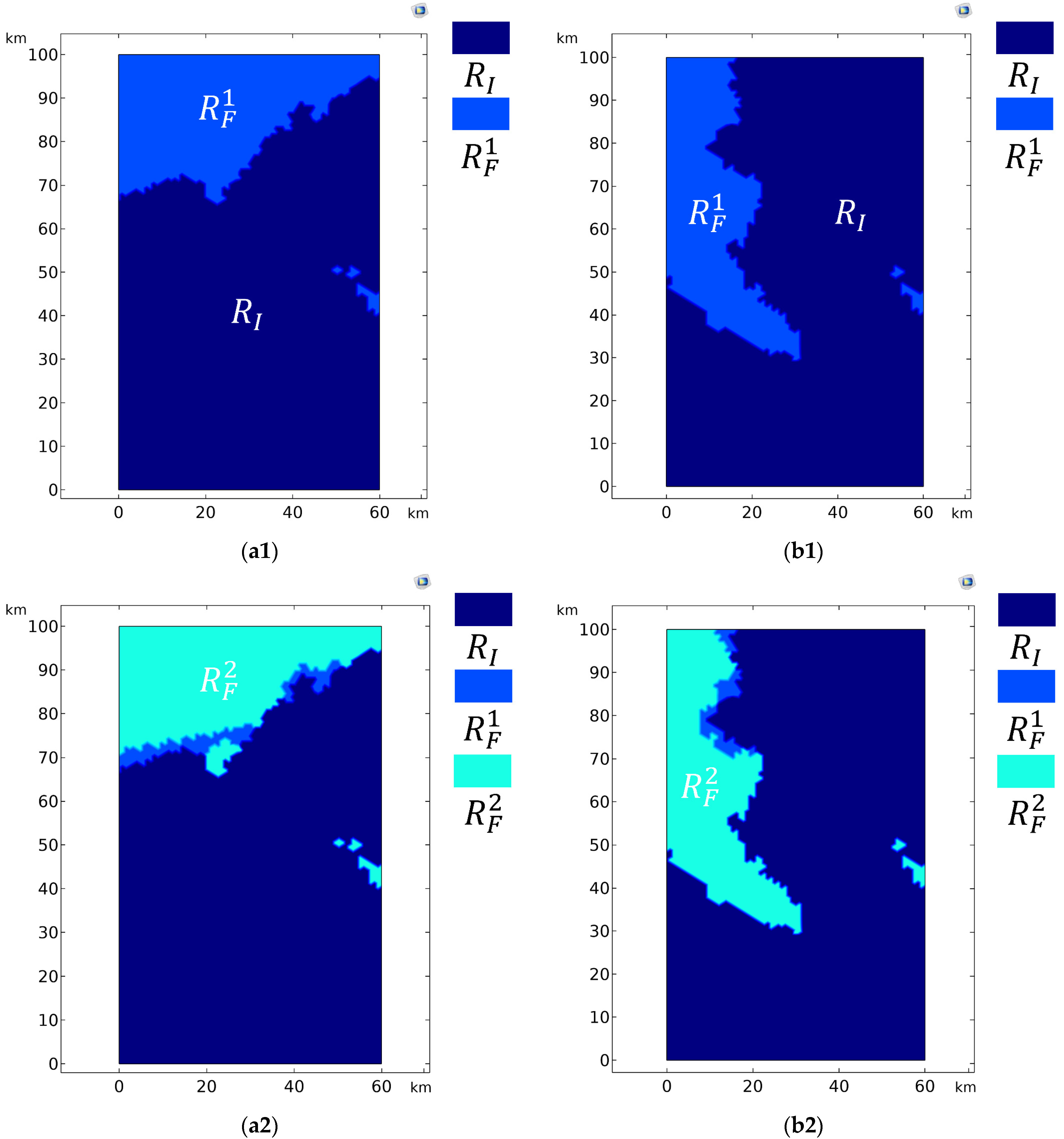
5.1. Arrangement Optimization of Two Stations
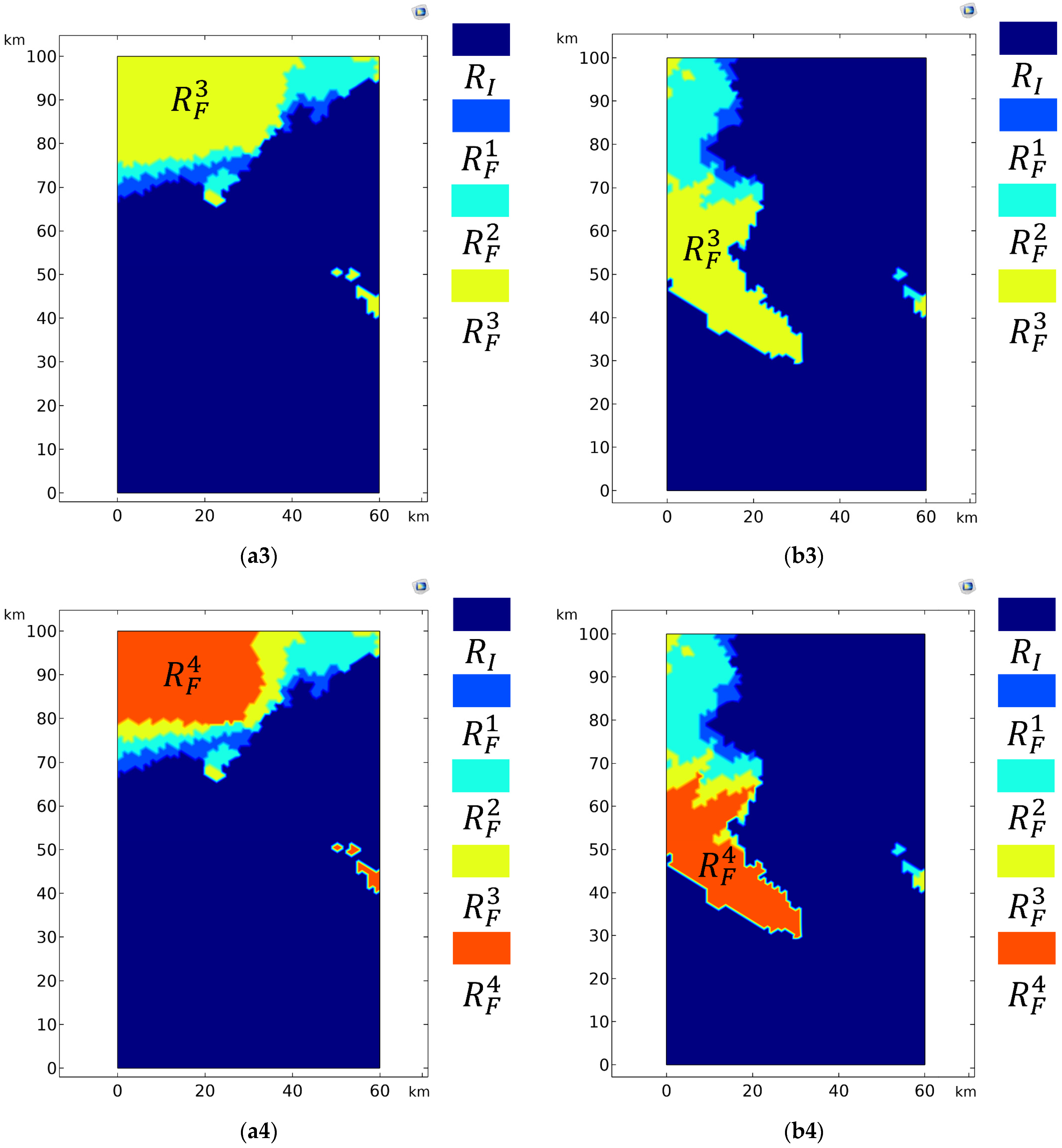
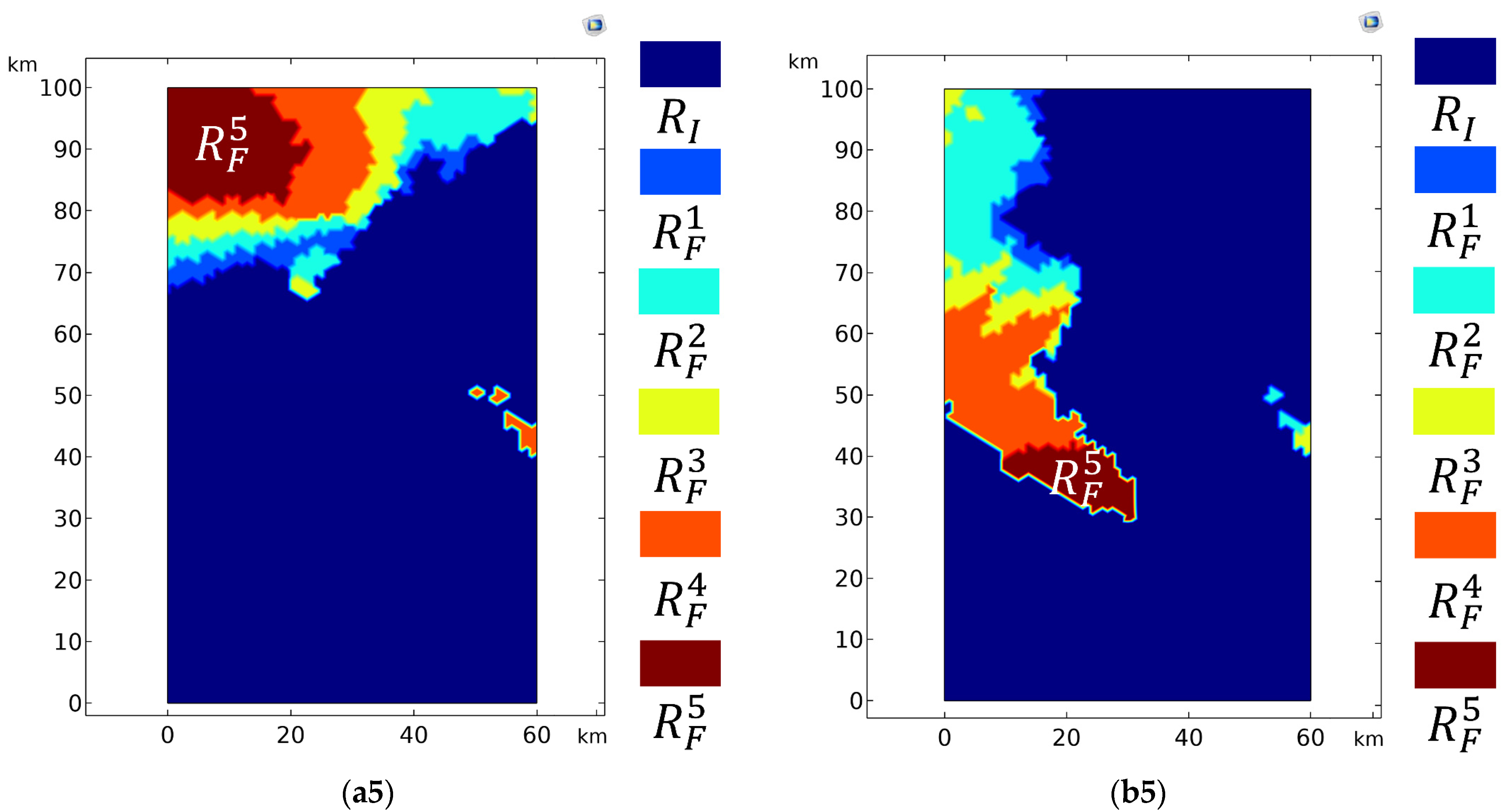
5.2. Relay Measurement with Multiple Stations
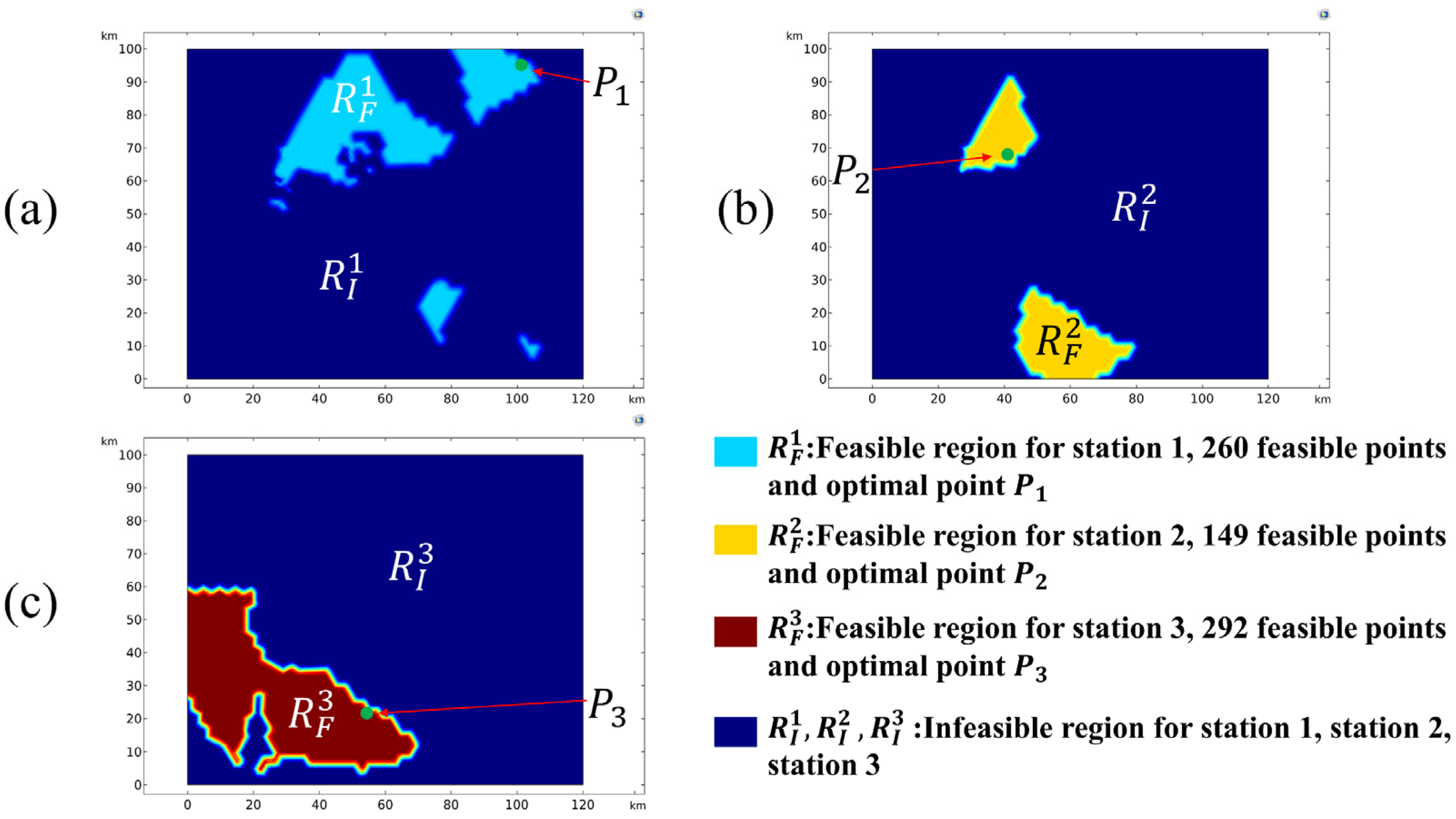
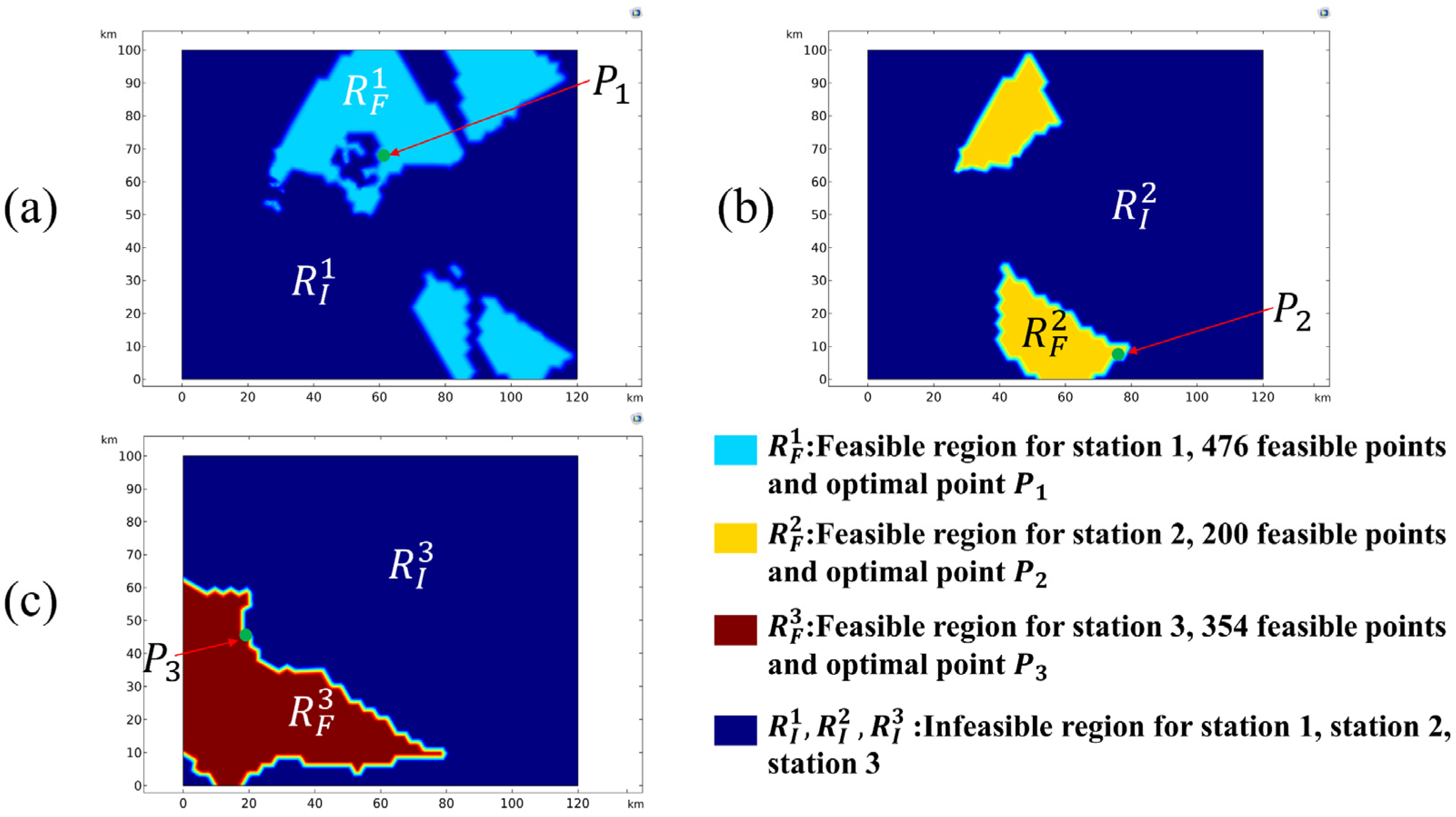
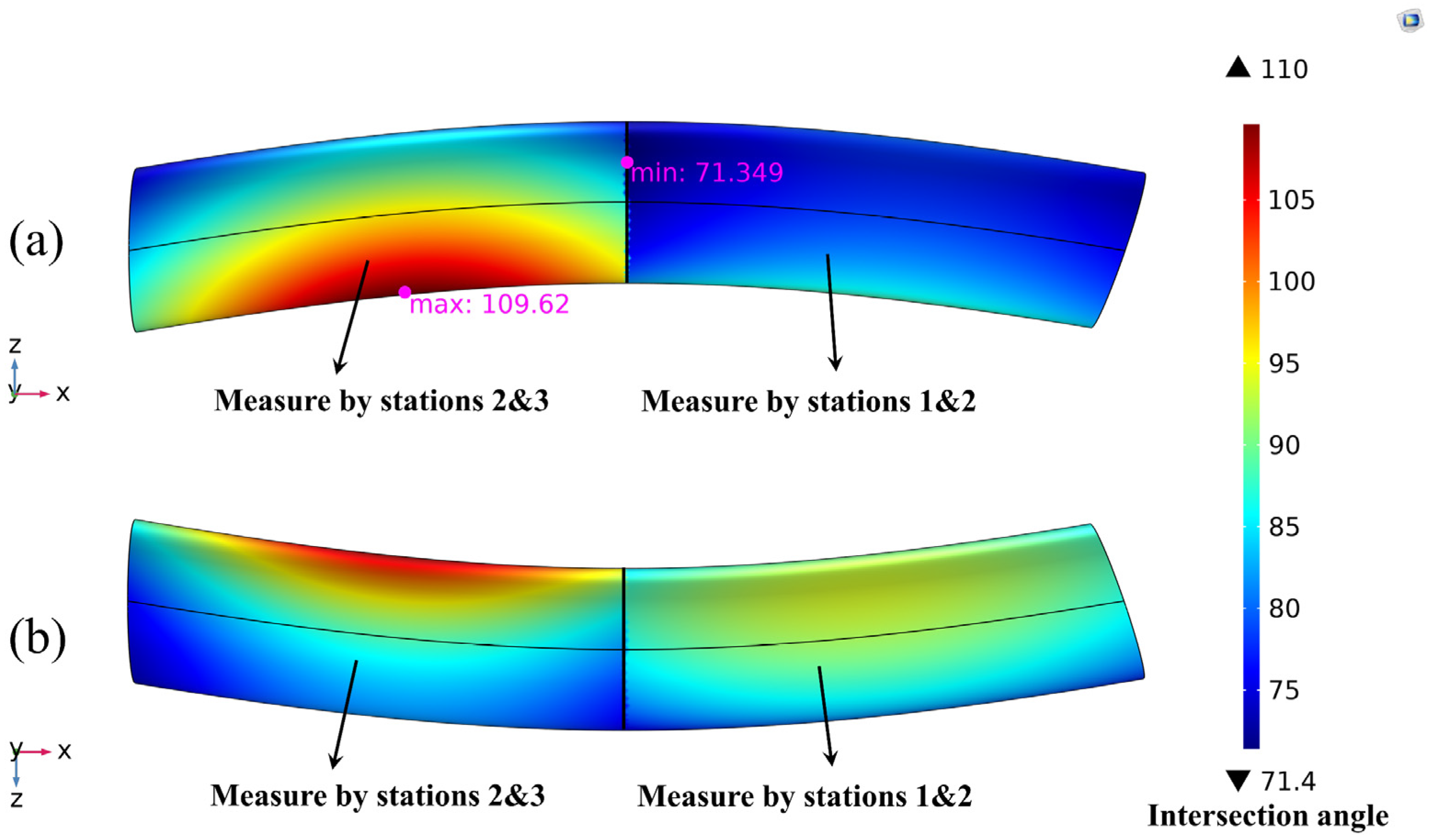
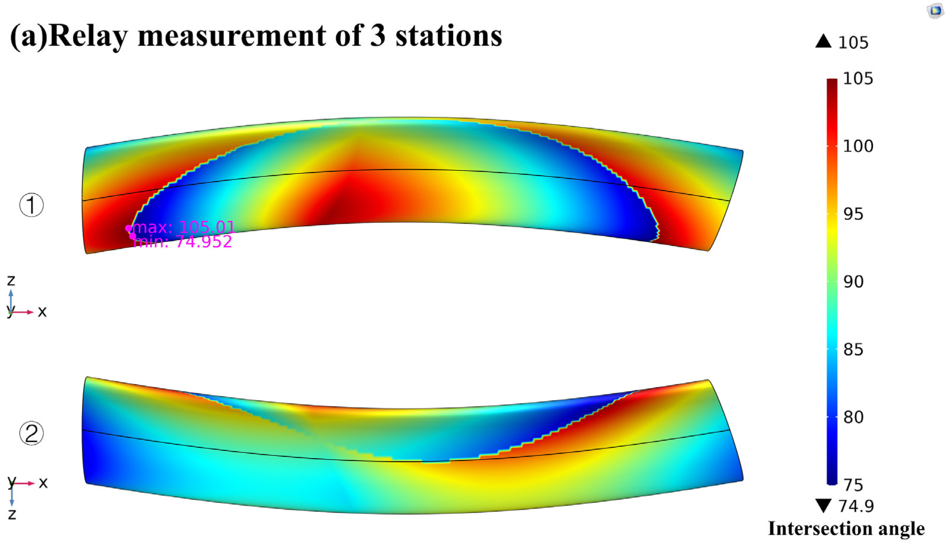
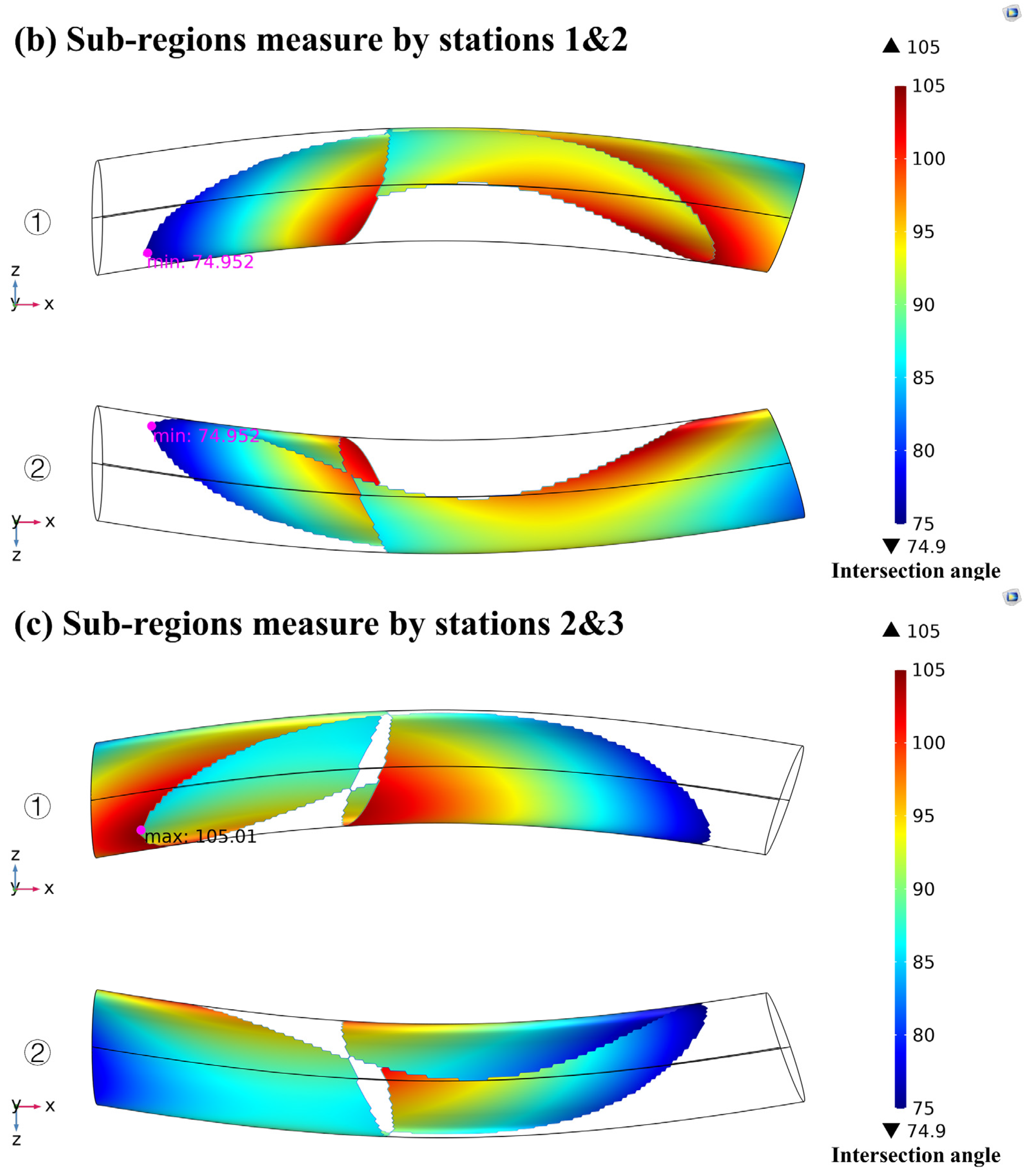
5.2.1. Relay Measurement of Three Stations
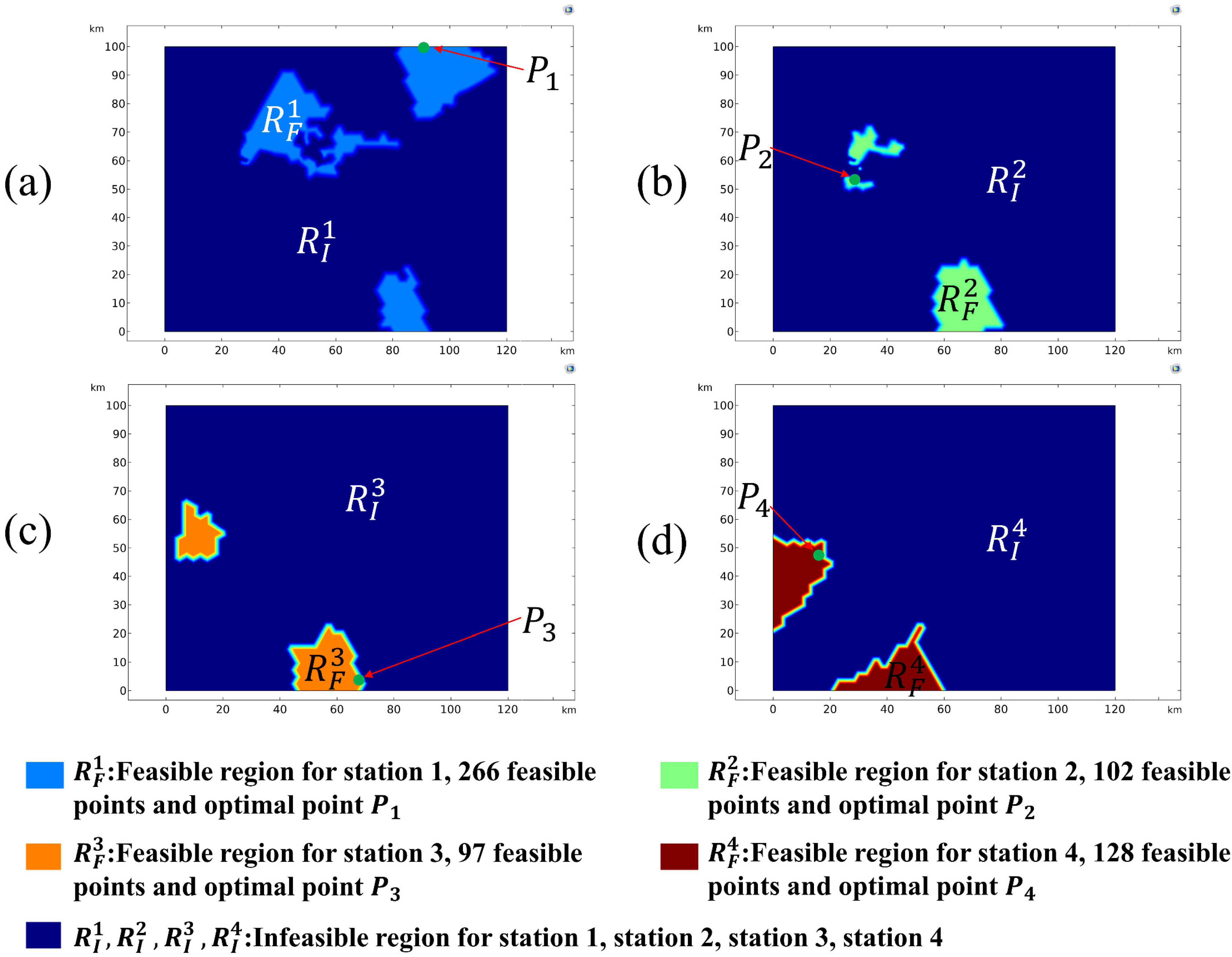
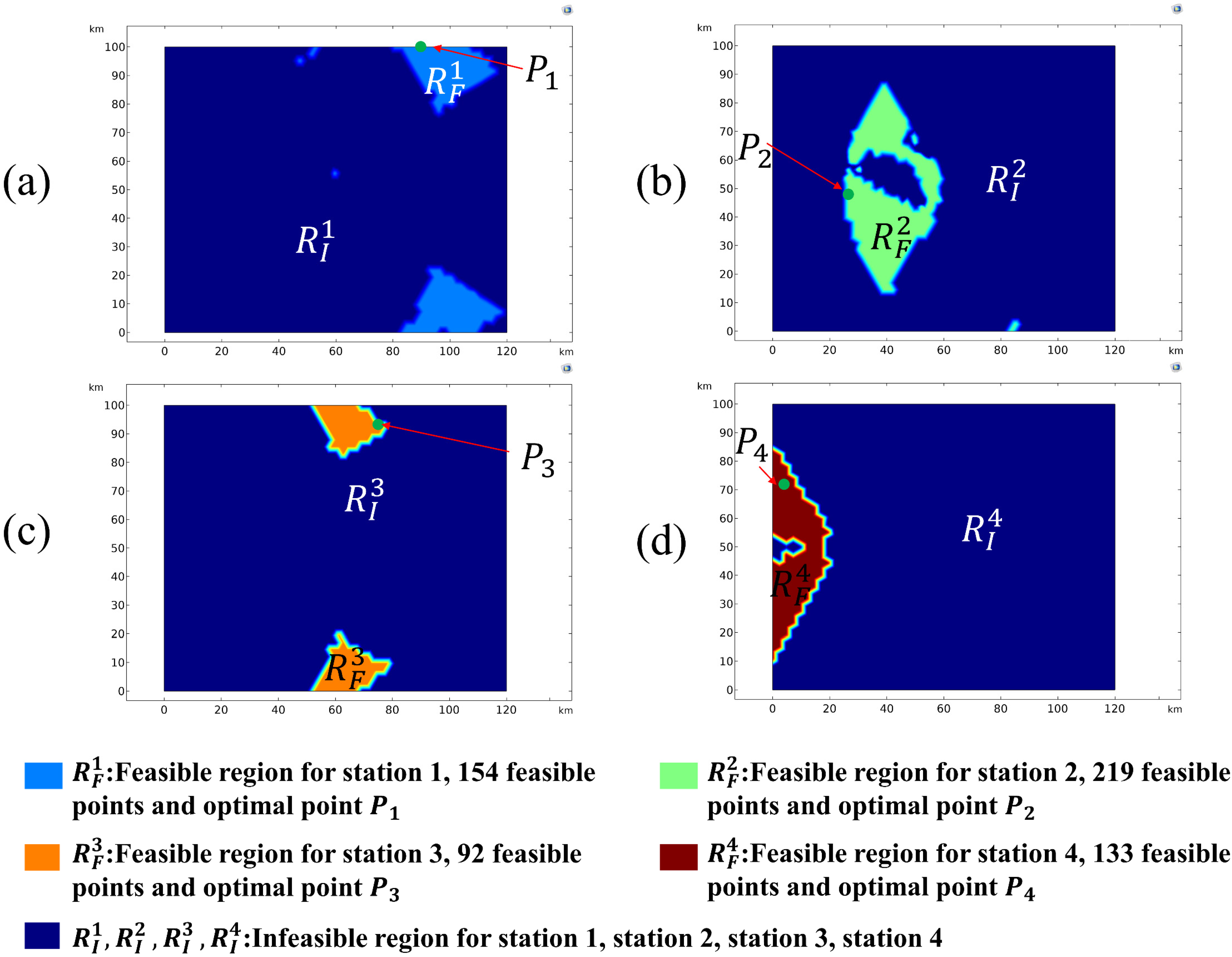
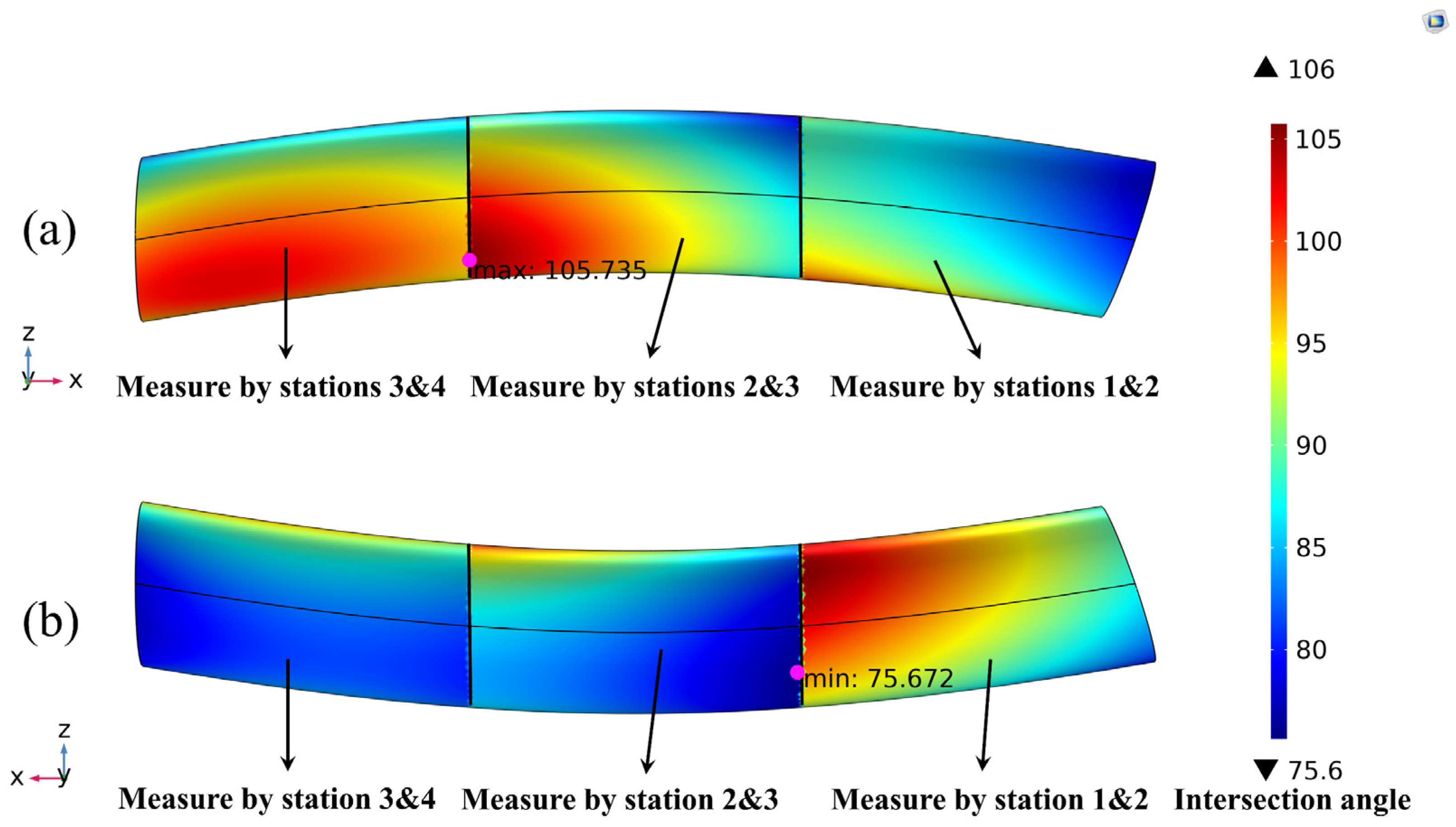
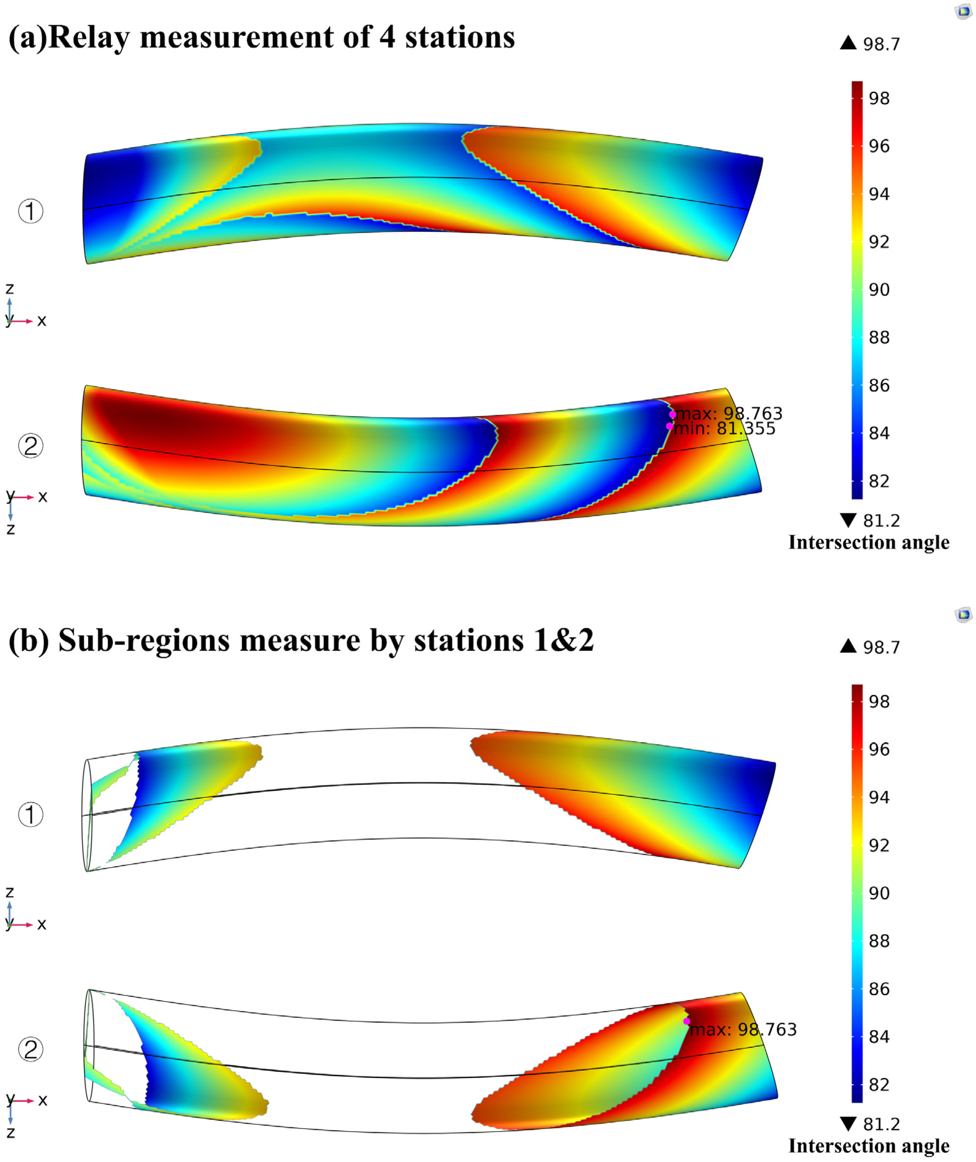
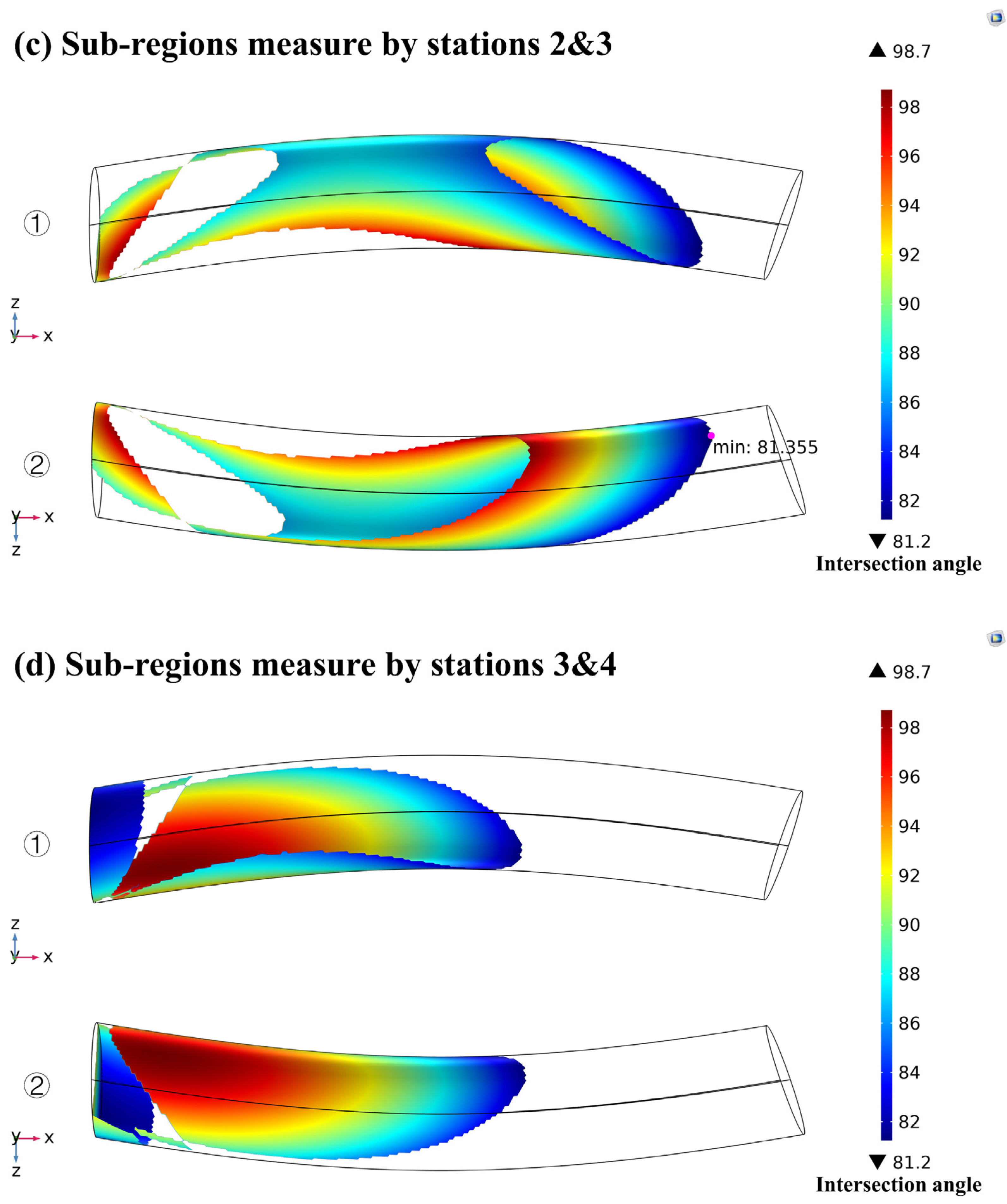
5.2.2. Relay Measurement of Four Stations
6. Conclusions
Author Contributions
Funding
Institutional Review Board Statement
Informed Consent Statement
Data Availability Statement
Conflicts of Interest
References
- Binghua, H.; Heng, W.; Hongli, H. A New Method of Trajectory Accurate Measurement by Single Photoelectric Theodolite. In Proceedings of the 2020 Chinese Automation Congress (CAC), Shanghai, China, 6–8 November 2020; pp. 4939–4943. [Google Scholar]
- Haomiao, L.; Wei, W.; Bile, W. Research on theodolite auto-collimation technique based on visual image analysis. In Proceedings of the 2017 IEEE 2nd Information Technology, Networking, Electronic and Automation Control Conference (ITNEC), Chengdu, China, 15–17 December 2017; pp. 150–153. [Google Scholar]
- Li, M. Concept Research on Stations Arrangement of Active Measurement System for More, Small, Rapid and Dark Objects; Chinese Academy of Sciences: Beijing, China, 2011. [Google Scholar]
- Bishop, A.N.; Fidan, B.; Anderson, B.D.O.; Pathirana, P.N.; Dogancay, K. Optimality Analysis of Sensor-Target Geometries in Passive Localization: Part 2—Time-of-Arrival Based Localization. In Proceedings of the 2007 3rd International Conference on Intelligent Sensors, Sensor Networks and Information, Melbourne, VIC, Australia, 6 March 2007; pp. 13–18. [Google Scholar]
- Zhong, Y.; Wu, X.Y.; Huang, S.C. Geometric dilution of precision for bearing-only passive location in three-dimensional space. Electron. Lett. 2015, 51, 518–519. [Google Scholar] [CrossRef]
- Xiu, J.J.; He, Y.; Wang, G.H.; Xiu, J.H.; Tang, X.M. Constellation of multisensors in bearing-only location system. IEE Proc.-Radar Sonar Navig. 2005, 152, 215–218. [Google Scholar] [CrossRef]
- Bai, J.; Wang, G.H.; Wang, N.; Xu, H. Study on Optimum Cut Angles in Bearing-only Location Systems. Acta Aeronaut. Astronaut. Sin. 2009, 30, 298–304. [Google Scholar]
- Yang, B.; Scheuing, J. Cramer-Rao bound and optimum sensor array for source localization from time differences of arrival. In Proceedings of the IEEE International Conference on Acoustics, Speech, and Signal Processing, Philadelphia, PA, USA, 23–23 March 2005; Volume 4, pp. iv/961–iv/964. [Google Scholar]
- Rui, L.; Ho, K.C. Elliptic localization: Performance study and optimum receiver placement. IEEE Trans. Signal Process. 2014, 62, 4673–4688. [Google Scholar] [CrossRef]
- Elhoseny, M.; Tharwat, A.; Farouk, A.; Hassanien, A.E. K-coverage model based on genetic algorithm to extend WSN lifetime. IEEE Sens. Lett. 2017, 1, 1–4. [Google Scholar] [CrossRef]
- Zameni, M.; Rezaei, A.; Farzinvash, L. Two-phase node deployment for target coverage in rechargeable WSNs using genetic algorithm and integer linear programming. J. Supercomput. 2021, 77, 4172–4200. [Google Scholar] [CrossRef]
- Hurley, S.; Khan, M.I. Netted radar: Network communications design and optimisation. Ad Hoc Netw. 2011, 9, 736–751. [Google Scholar] [CrossRef]
- Guo, L.; Zhu, Y.; Di, Y. Optimization of photoelectric theodolite station distribution based on GA. Chin. J. Sci. Instrum. 2010, 31, 741–746. [Google Scholar]
- Yang, L.; Xiong, J.; Jian, C. Method of Optimal Deployment for Radar Netting Based on Detection Probability. In Proceedings of the 2009 International Conference on Computational Intelligence and Software Engineering, Wuhan, China, 11–13 December 2009; pp. 1–5. [Google Scholar]
- Yi, J.; Wan, X.; Leung, H. Receiver placement in multistatic passive radars. In Proceedings of the 2015 IEEE Radar Conference (RadarCon), Arlington, VA, USA, 10–15 May 2015; pp. 0876–0879. [Google Scholar]
- Lin, F.; Chiu, P.L. A near-optimal sensor placement algorithm to achieve complete coverage-discrimination in sensor networks. IEEE Commun. Lett. 2005, 9, 43–45. [Google Scholar]
- Zhang, H.; Zhang, S.; Bu, W. A clustering routing protocol for energy balance of wireless sensor network based on simulated annealing and genetic algorithm. Int. J. Hybrid Inf. Technol. 2014, 7, 71–82. [Google Scholar] [CrossRef]
- Zhang, T.; Liang, J.; Yang, Y.; Cui, G.; Kong, L.; Yang, X. Antenna deployment method for multistatic radar under the situation of multiple regions for interference. Signal Process. 2018, 143, 292–297. [Google Scholar] [CrossRef]
- Wang, Y.; Yi, W.; Yang, S.; Mallick, M.; Kong, L. Antenna Placement Algorithm for Distributed MIMO Radar with Distance Constrains. In Proceedings of the 2020 IEEE Radar Conference (RadarConf20), Florence, Italy, 21–25 September 2020; pp. 1–6. [Google Scholar]
- Jin, G.; Wang, J.Q.; Wei, N.I. The Three error Axis of Theodolite with the Utilization of the Coordinate to the Variation. Opt. Precis. Eng. 1999, 05, 89–94. [Google Scholar]
- Huang, B.; Li, Z.H.; Tian, X.Z.; Yang, L.; Zhang, P.J.; Chen, B. Modeling and correction of pointing error of space-borne optical imager. Optik 2021, 247, 167998. [Google Scholar] [CrossRef]
- Li, H.; Hu, Y. Correction method for photoelectric theodolite measure error based on BP neural network. In Proceedings of the Intelligent Computing and Information Science: International Conference, ICICIS 2011, Chongqing, China, 8–9 January 2011; Proceedings, Part I. Springer: Berlin/Heidelberg, Germany, 2011; pp. 225–230. [Google Scholar]
- Zhao, L.; Zhu, W.; Zhang, Y.; Sun, J. The method of the system error modification of photoelectric theodolite of T type. In Proceedings of the 2012 International Conference on Optoelectronics and Microelectronics, Florence, Italy, 21–25 September 2012; pp. 384–387. [Google Scholar]
- Calafiore, G. Reliable localization using set-valued nonlinear filters. IEEE Trans. Syst. Man Cybern.—Syst. Hum. 2005, 35, 189–197. [Google Scholar] [CrossRef]
- Jia, T.; Wu, N.-W.; Chen, T. Cramer-Rao lower bounds of position estimation in a photoelectric theodolite-based network. Opto-Electron. Eng. 2005, 07, 4–6+18. [Google Scholar]
- Farina, A. Target tracking with bearings-only measurements. Signal Process. 1999, 78, 61–78. [Google Scholar] [CrossRef]
- Fisher, P.F.; Tate, N.J. Causes and consequences of error in digital elevation models. Prog. Phys. Geogr. 2006, 30, 467–489. [Google Scholar] [CrossRef]
- Holmes, K.W.; Chadwick, O.A.; Kyriakidis, P.C. Error in a USGS 30-meter digital elevation model and its impact on terrain modeling. J. Hydrol. 2000, 233, 154–173. [Google Scholar] [CrossRef]
- Alfakih, A.Y.; Charron, P.; Piccialli, V.; Wolkowicz, H. Euclidean Distance Matrices, Semidefinite Programming, and Sensor Network Localization. Port. Math. 2011, 68, 53–102. [Google Scholar] [CrossRef] [PubMed]
- Dokmanic, I.; Parhizkar, R.; Ranieri, J.; Vetterli, M. Euclidean Distance Matrices: A Short Walk Through Theory, Algorithms and Applications. IEEE Signal Process. Mag. 2015, 32, 12–30. [Google Scholar] [CrossRef]
- Drusvyatskiy, D.; Krislock, N.; Voronin, Y.L.; Wolkowicz, H. Noisy Euclidean distance realization: Robust facial reduction and the Pareto frontier. Mathematics 2015, 27, 2301–2331. [Google Scholar] [CrossRef]


| Traverse Coarse Grids | Local Refinement | Local Optimization | |
|---|---|---|---|
| Coordinate of station 1 | (2.1680, 88.7057, 1.5034) | (0, 89.5230, 1.4786) | (0, 89.5249, 1.4742) |
| Coordinate of station 2 | (27.1074, 33.0486, 1.537) | (26.6280, 31.731, 1.5403) | (26.6297, 31.731, 1.5394) |
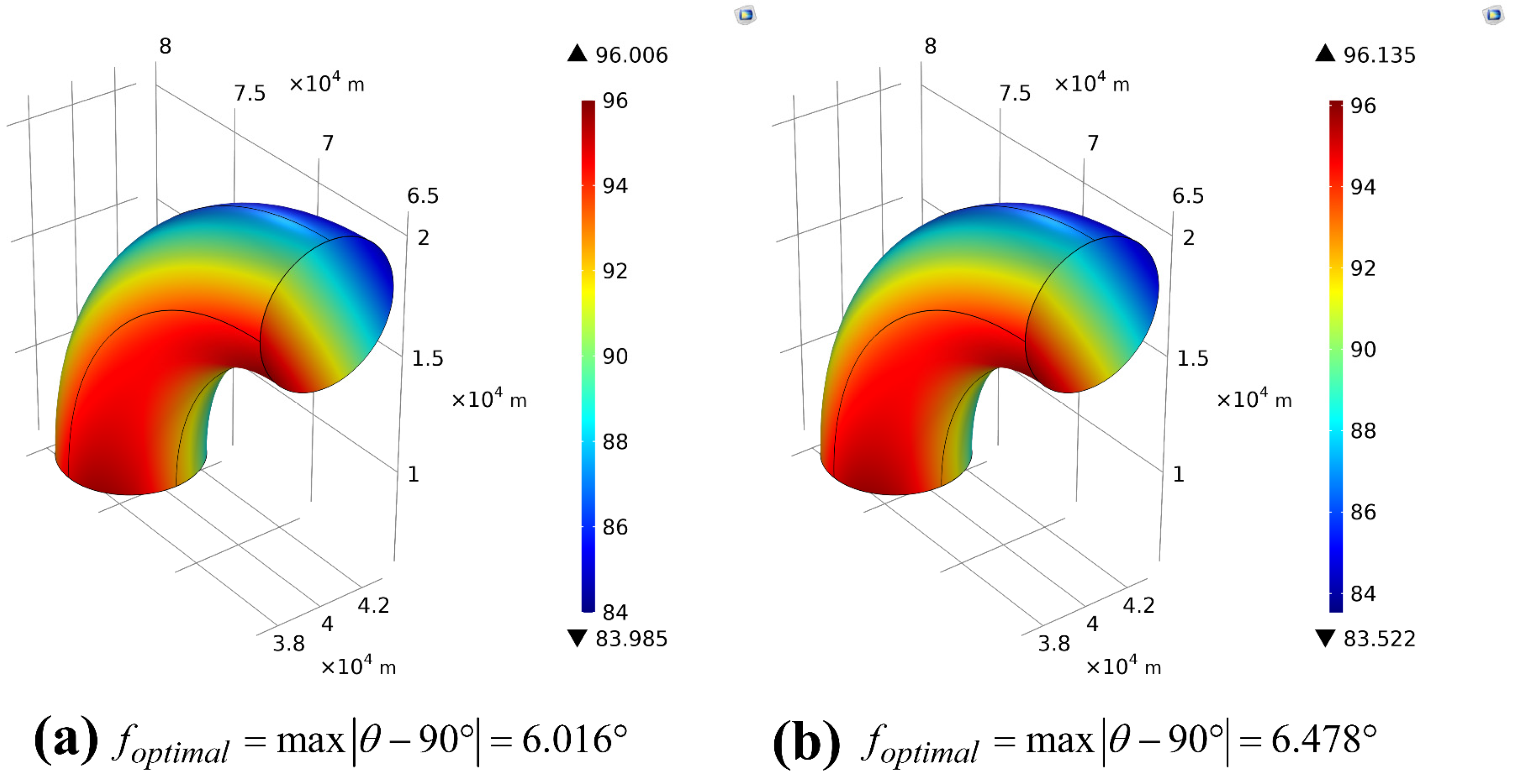
| Intersection angle range | 83.522–96.135° | 83.994–96.023° | 83.984–96.006° |
| Value of objective function | 6.478 | 6.023 | 6.016 |
| Traditional Relay Mode | Second Relay Mode | |
|---|---|---|
| Coordinate of station 1 | (103.257, 95.156, 1.562) | (59.051, 66.253, 2.015) |
| Coordinate of station 2 | (42.457, 65.810, 2.098) | (77.428, 8.507, 2.021) |
| Coordinate of station 3 | (54.364, 21.794, 1.836) | (19.760, 44.910, 1.498) |
| Intersection angle range | 71.356–109.632° | 74.952–105.007° |
| Value of objective function | 19.632 | 15.048 |
| Traditional Relay Mode | Second Relay Mode | |
|---|---|---|
| Coordinate of station 1 | (92.093, 100.00, 1.583) | (91.152, 100.00, 1.583) |
| Coordinate of station 2 | (28.163, 53.536, 1.772) | (28.391, 48.014, 1.630) |
| Coordinate of station 3 | (66.943, 0, 2.241) | (77.040, 93.501, 1.452) |
| Coordinate of station 4 | (16.934, 45.761, 1.491) | (2.579, 72.823, 1.644) |
| Intersection angle range | 75.672–105.735° | 81.355–98.763° |
| Value of objective function | 15.735 | 8.763 |
Disclaimer/Publisher’s Note: The statements, opinions and data contained in all publications are solely those of the individual author(s) and contributor(s) and not of MDPI and/or the editor(s). MDPI and/or the editor(s) disclaim responsibility for any injury to people or property resulting from any ideas, methods, instructions or products referred to in the content. |
© 2023 by the authors. Licensee MDPI, Basel, Switzerland. This article is an open access article distributed under the terms and conditions of the Creative Commons Attribution (CC BY) license (https://creativecommons.org/licenses/by/4.0/).
Share and Cite
Miao, Z.; Li, Y.; Wang, C.; Yu, Y.; Liu, Z. Station Arrangement Optimization of Photoelectric Theodolites Based on Efficient Traversing Discrete Points. Photonics 2023, 10, 870. https://doi.org/10.3390/photonics10080870
Miao Z, Li Y, Wang C, Yu Y, Liu Z. Station Arrangement Optimization of Photoelectric Theodolites Based on Efficient Traversing Discrete Points. Photonics. 2023; 10(8):870. https://doi.org/10.3390/photonics10080870
Chicago/Turabian StyleMiao, Zhenyu, Yaobin Li, Chong Wang, Yi Yu, and Zhenyu Liu. 2023. "Station Arrangement Optimization of Photoelectric Theodolites Based on Efficient Traversing Discrete Points" Photonics 10, no. 8: 870. https://doi.org/10.3390/photonics10080870
APA StyleMiao, Z., Li, Y., Wang, C., Yu, Y., & Liu, Z. (2023). Station Arrangement Optimization of Photoelectric Theodolites Based on Efficient Traversing Discrete Points. Photonics, 10(8), 870. https://doi.org/10.3390/photonics10080870