Adaptive Weighted K-Nearest Neighbor Trilateration Algorithm for Visible Light Positioning

Abstract

An adaptive weighted K-nearest neighbor (AWKNN) trilateration positioning algorithm fused with the channel state information (CSI) is proposed to optimize the accuracy of the visible light positioning. The core concept behind this algorithm is to combine the WKNN algorithm with ranging based on the CSI. The direct path distance estimated by the CSI is utilized to construct a position set consisting of multiple positions and a corresponding distance database containing multiple distance vectors. The error parameters of the weighted combinations of different distance vectors are calculated iteratively to evaluate the impact of different K-values and weights on the positioning accuracy. The proposed algorithm can achieve high-precision trilateration positioning by adaptively selecting the K-value and weight. A typical 4 m × 4 m × 3 m indoor multipath scene with four LEDs is established to simulate the positioning performance. The simulation results reveal that the mean error of the CSI-based AWKNN algorithm achieves 1.84 cm, with a root mean square error (RMSE) of 2.13 cm. Compared with the CSI-based least squares (LS) method, the CSI-based nonlinear LS method, and the CSI-based WKNN method, the average error of this method is decreased by 29%, 16%, and 17%, whereas the RMSE is reduced by 35%, 14%, and 19%.

1. Introduction

Today, the majority of indoor Internet of Things (IoT) application scenarios rely on high-precision location services, such as the navigation of automated guided vehicles (AGVs) in smart factories, picking in smart warehouses, and tracking in underground garages. Therefore, research on indoor positioning technology has become a prominent topic [1,2]. The existing common indoor positioning technologies, radio frequency identification (RFID), WiFi, and Bluetooth are susceptible to the interference of indoor multipath effects and cannot achieve good positioning in complex indoor scenes [3]. Visible light positioning (VLP) has become a promising high-precision positioning technology due to its advantages of being license-free, having low power consumption, and having anti-electromagnetic interference [4]. The indoor VLP algorithms include the received signal strength (RSS) [5,6], angle of arrival (AOA) [7], time of arrival (TOA) [8], time difference of arrival (TDOA) [9], etc. Among them, the RSS-based VLP has been widely investigated because of its low hardware requirements and easy implementation.

In recent years, various RSS-based VLP trilateration algorithms have been developed, such as an improved whale optimization algorithm for 3D positioning systems [10], a received signal strength-assisted perspective three-point positioning algorithm (R-P3P) [11], and gradient descent (GD)–least squares (LS) and iterative LS algorithms [12]. However, these studies did not consider the influence of the reflection path. A nonlinear estimation method based on the RSS was proposed to reduce the influence of the multipath reflection [13]. However, this method did not use multipath channel information, resulting in only submeter positioning accuracy. In our previous work [14], a trilateration positioning method based on channel state information (CSI) was investigated, which can effectively reduce the interference of reflected paths on distance measurements, thereby significantly improving localization performance. However, the optimization of the estimation error in the LS algorithm was not considered. Fingerprinting algorithms in VLP have also received a lot of attention, including the weighted K-nearest neighbor (WKNN) [15], the weighted optimum KNN (WOKNN) [16], and the adaptive residual WKNN (ARWKNN) [17]. However, these methods require high-cost offline data acquisition and map construction, and their performance is largely affected by the spatial distribution of sampling points.

To achieve high-accuracy and highly robust localization, many visible light fusion localization methods combined with machine learning (ML) have been investigated, such as the residual concatenation neural network (RCNN) [18], the long short-term memory–fully connected network (LSTM-FCN) [19], the convolutional neural network (CNN) [20], the memory artificial neural network (M-ANN) [21], the position estimation deep neural network (PE-DNN) [22], and a combination of extreme learning machine (ELM) and density-based spatial clustering of applications with noise (DBSCAN) [23]. However, these algorithms require a lot of preprocessing for specific scenarios, resulting in poor generality and high cost.

Considering the issues of the above VLP schemes, a high-precision adaptive WKNN (AWKNN) trilateration positioning algorithm fusing the CSI is presented in this paper, which does not require offline data acquisition and data training. The main contributions of this paper are as follows:

(1) This paper innovatively combines CSI-based ranging with WKNN to solve the nonlinear error problem in VLP trilateration positioning. With the help of CSI-based ranging, the WKNN is provided with high-quality location sets and distance databases, and fingerprint matching is converted into a distance vector difference calculation to achieve an adaptive selection of K-values and corresponding weights.

(2) Some works ignore the interference of the reflected signals in VLP systems, which is the main challenge for accurate distance measurements. In this study, an indoor multipath simulation scene is employed to analyze the positioning accuracy and computational complexity of the proposed algorithm. The simulation results show that the localization accuracy of the AWKNN algorithm in the whole room, edge area, and center area is better than that of the comparison methods, which verifies the effectiveness of the proposed method. In addition, the influence of the signal-to-noise ratio (SNR) on the positioning accuracy of CSI-based trilateration positioning methods is also analyzed.

The rest of this paper is organized as follows: Section 2 describes the system model and related work. The AWKNN method is proposed in Section 3. The simulation results of the positioning performance are presented and analyzed in Section 4. The conclusions are discussed in Section 5.

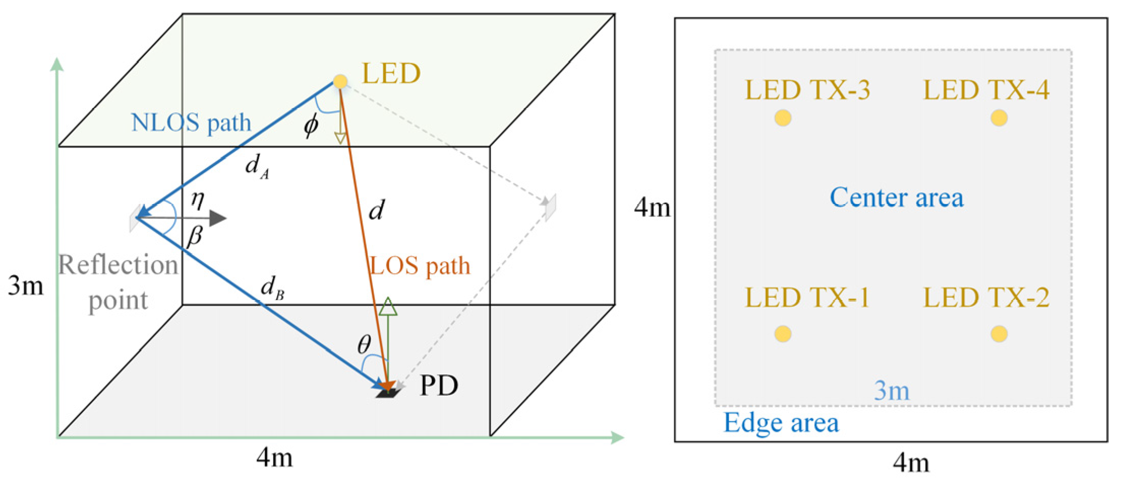
2. System Model

2.1. Optical Wireless Channel Model

The model of a typical indoor simulation scene with a size of 4 m × 4 m × 3 m is illustrated in Figure 1, including four LEDs as transmitters and one PD as a receiver. The four LEDs (TX1–4) are arranged on the top of the room to send positioning signals, including coordinate information and emitted light power. The LEDs’ horizontal coordinates are (1,1), (1,3), (3,1), and (3,3). The center area is the area enclosed by the dotted line in Figure 1, which is a 3 m × 3 m square area in the center of the room, and the area outside the dotted line is the edge area.

Observing Figure 1, it can be seen that the signal received by the PD includes the line-of-sight (LOS) signal and a large number of non-line-of-sight (NLOS) signals produced by reflection. Therefore, in the optical channel model in this paper, the total channel gain is considered the sum of the LOS path gain and the first-order reflected path gain. The discrete-time channel impulse response (CIR), consisting of the LOS path gain and several discrete NLOS path gains, is expressed as

$$\mathrm{h}=\left[\begin{array}{cccc}h(0)& h(1)& \cdots & h(L-1)\end{array}\right],$$

(1)

where L denotes the number of channel paths. The discrete NLOS path gains are generated by summarizing those reflected path gains delayed over one sampling interval, and the l-th path gain is exhibited as [14]

$$h(l)=\left\{\begin{array}{l}{h}_{LOS}\hspace{0.33em}\hspace{0.33em}\hspace{0.33em}\hspace{0.33em}\hspace{0.33em}\hspace{0.33em}\hspace{0.33em}\hspace{0.33em}\hspace{0.33em}\hspace{0.33em}\hspace{0.33em}\hspace{0.33em}\hspace{0.33em}\hspace{0.33em}\hspace{0.33em}\hspace{0.33em}\hspace{0.33em}\hspace{0.33em}l=0\\ {\displaystyle {\int }_{{\tau }_0+(l-1)\cdot T_s}^{{\tau }_0+l\cdot T_s}{h}_{Ref}(t)dt,\hspace{0.33em}\hspace{0.33em}\hspace{0.33em}\hspace{0.33em}1\le l\le L-1}\end{array}\right.,$$

(2)

where ${\tau }_0$ denotes the arrival time of the LOS path signal, $T_s$ indicates the sampling interval, $h_{LOS}$ represents the LOS path channel gain, and $h_{Ref}(t)$ represents the reflection path channel gain. The channel gain of the LOS path can be given by [14]

$$h_{LOS}=\frac{(m+1)A_{PD}}{2\pi d^2}{\cos }^m(\varphi )T_s(\theta )g(\theta )\cos (\theta ),$$

(3)

where $m$ is the order of the Lambertian emission, $A_{PD}$ denotes the effective area of the PD, $d$ reflects the distance from the LED to the PD, $\theta$ is the PD’s incident angle, and $\varphi$ is the LED’s irradiance angle. $g(\theta )$ is the gain of the optical concentrator, and $T_s(\theta )$ is the gain of the optical filter.

The reflection path channel gain can be obtained by [14]

$$h_{ref}(t)=\frac{(m+1)A\rho A_{wall}}{2{\pi }^2{d}_A{}^2{d}_B{}^2}{\cos }^m(\varphi )\cos (\eta )\cos (\beta )T_s(\theta )g(\theta )\cos (\theta ),$$

(4)

where $\rho$ is the reflection coefficient of the wall, $A_{wall}$ depicts the area of the reflection point, $d_A$ denotes the distance from the LED to a reflection point, $d_B$ presents the distance from a reflection point to the PD, $\eta$ is the incident angle of a reflection point, and $\beta$ indicates the irradiance angle to the PD.

The optical signal intensity transmitted by the LED is denoted as $P_t$, and the optical intensity $P_r$ received by the PD can be illustrated as [14]

$$P_r=P_t\cdot {\displaystyle \sum _{l=0}^{L-1}h(l)}.$$

(5)

2.2. CSI-Based Positioning System Model

In CSI-based VLP systems, time-division multiple access (TDMA) is employed as a data transmission scheme to prevent signals of different LEDs from interfering with each other. The positioning signal transmitted by the LED, including the synchronization symbol, pilot symbol, and data symbol, is modulated by DC offset optical OFDM (DCO-OFDM). For details on localization signal generation, kindly refer to our previous work [14].

The baseband signal received by the PD can be expressed as

$$r(n)=h(n)\otimes x(n)+w(n),$$

(6)

where $h(n)$ indicates the CIR, and $\otimes$ denotes the convolution. $w(n)$ represents the additive white Gaussian noise (AWGN), including the shot noise and thermal noise.

At the receiver, to ensure the correct extraction of the pilot symbols and accurate channel estimation, the timing synchronization algorithm described in [24] is employed to estimate the beginning position of the DCO-OFDM symbols. The received frequency-domain pilot sequence can be expressed as [14]

$$\widehat{\mathrm{X}} =\left[{\widehat{X}}_0^{} {\widehat{X}}_1^{}\cdots {\widehat{X}}_{N_P/2-1}^{} {\widehat{X}}_{N_P/2}^{} {\left({\widehat{X}}_{N_P/2-1}^{}\right)}^{*}\cdots {\left({\widehat{X}}_1^{}\right)}^{*} \right]\hspace{0.33em}=\mathrm{H}\cdot \mathrm{X}+\mathrm{W},$$

(7)

where $N_P$ indicates the length of the pilot symbol, $\mathrm{H}$ denotes the channel frequency response (CFR), and $\mathrm{X}$ represents the pilot sequence saved locally.

The CFR is estimated using the LS algorithm, and the estimated CFR can be obtained by [14]

$$\widehat{\mathrm{H}} = \widehat{\mathrm{X}}/\mathrm{X}=\left[0 {\widehat{X}}_1^{}/X_1^{} \cdots {\widehat{X}}_{N_P/2-1}^{}/X_{N_P/2-1}^{} 0 {\left({\widehat{X}}_{N_P/2-1}^{}\right)}^{*}/X_{N_P/2-1}^{*} \cdots {\left({\widehat{X}}_1^{}\right)}^{*}/X_1^{*}\right].$$

(8)

IFFT is then performed on the CFR to obtain the real-valued CIR, denoted as $\widehat{\mathrm{h}}$. Since the estimated CIR vector is affected by noise, resulting in a negative gain of some paths, which is inconsistent with the fact that the channel gain in the actual scene is positive, the negative values in the CIR vector should be clipped to 0, denoted as ${ \widehat{\mathrm{h}} }_{\mathrm{clip}}=\max (0, \widehat{\mathrm{h}} )$.

To estimate the ratio of the LOS path to the total path, the method for estimating the number of channel paths from the preceding work is utilized [14]. The received power of the LOS signal is expressed as

$${\widehat{P}}_{rLOS}={\widehat{P}}_r\cdot {\widehat{h}}_{LOS}={\widehat{P}}_r\cdot {\widehat{h}}_{clip}(0)/{\displaystyle \sum _{l=0}^{T-1}{\widehat{h}}_{clip}(l)},$$

(9)

where $T$ is the estimated number of channel paths. We assume that the LED and the PD are placed in parallel. To put it another way, $\cos (\varphi )=\cos (\theta )=H/d$, where $H$ is the vertical height between the LED and the PD. We assume that the number of LEDs is $N$, and the LOS path distance $d_{LOS,i}$ between the PD and the i-th LED can be calculated as

$$d_{LOS,i}=\sqrt[m+3]{\frac{(m+1)\cdot A_{PD}\cdot T_S(\theta )\cdot g(\theta )\cdot H^{m+1}\cdot P_{t,i}}{2\pi \cdot {\widehat{P}}_{rLOS,i}}}\begin{array}{cc}& (1\le i\le N)\end{array}.$$

(10)

Then, the relationship between the coordinate $(x,y)$ of the PD and the coordinate $(x_i,y_i)$ of the LED is as follows.

$$\left\{\begin{array}{c}{\left(x-x_1\right)}^2+{\left(y-y_1\right)}^2=d_{LOS,1}^2-H^2\\ ⋮\\ {\left(x-x_N\right)}^2+{\left(y-y_N\right)}^2=d_{LOS,N}^2-H^2\end{array}\right..$$

(11)

2.3. Related Work

2.3.1. Nonlinear LS Estimation Algorithm

The nonlinear LS estimation algorithm is briefly introduced below. The position estimated by the LS method is first selected as the initial position. Then, the M points around the initial position are selected to construct a position set and calculate the distance difference using Equation (12), where the position with the smallest difference value is used as the center position of the next iteration [13].

$$S_j=\sqrt{{\displaystyle \sum _{i=1}^N{(\sqrt{{(x_i-x_j^{\prime })}^2+{(y_i-y_j^{\prime })}^2}-r_i)}^2}} j=1,\dots ,M,$$

(12)

where $(x_j^{\prime },y_j^{\prime })$ represents the j-th coordinate in the position set, $(x_i,y_i)$ represents the coordinate of the i-th LED, and $r_i$ is the estimated horizontal distance.

In the next iteration process, the M points around the center position are also selected to construct a position set. After T iterations, the final estimated position is obtained.

2.3.2. Modified WKNN Algorithm

The WKNN algorithm presented in [15] is specially designed for fingerprint positioning and relies on the matching of online collected data and offline fingerprint database; so, it needs to be modified for the trilateration positioning system. First, a location set consisting of M points is constructed in a similar way to the NLS method above, and the distance difference is calculated using Equation (12).

Then, the K positions with the smallest difference are taken as the K-nearest neighbors. The smallest K differences are denoted as $\left[\begin{array}{cccc}{S}_1^{\prime }& S_2^{\prime }& \cdots & S_K^{\prime }\end{array}\right]$. The weight of the modified WKNN is defined as

$$w_k=1/S_k^{\prime }/\left({\displaystyle \sum _{p=1}^{K}1/S_p^{\prime }}\right)\begin{array}{cc}& k=1,\cdots ,K\end{array}.$$

(13)

Finally, the output coordinate is obtained by using the weight and the K-nearest neighbors.

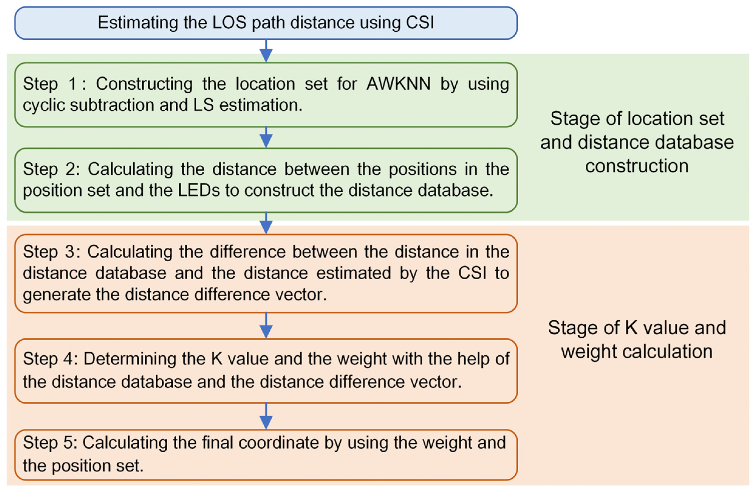
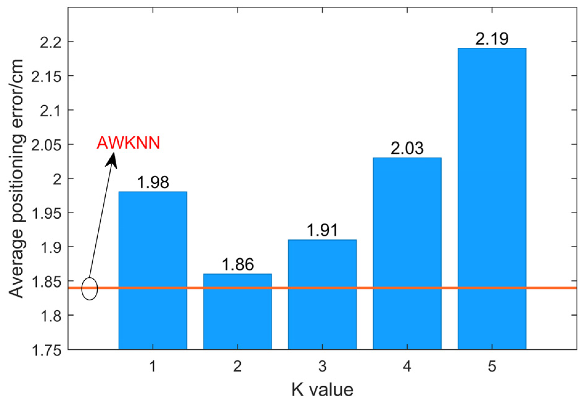
3. AWKNN Method

To reduce the nonlinear error in the trilateration positioning, this paper draws on the idea of the ARWKNN fingerprint positioning algorithm [17] and proposes an AWKNN positioning algorithm incorporating the CSI, which adaptively selects the K-value and weight to obtain excellent positioning accuracy. The schematic diagram of the AWKNN method based on the CSI is shown in Figure 2. The implementation of the AWKNN algorithm includes two stages: the stage of the location set and distance database construction, and the stage of the K-value and weight calculation. Following are the specific steps of the algorithm.

Step 1. Construction of the location set: Observing Equation (14), the LS method uses only one equation for subtraction with the rest, which leads to data waste and underutilizes the equations. Therefore, in this section, a cyclic subtraction is used to obtain several different locations as the initial position set for the AWKNN algorithm. The k-th position $(x_k^{\prime },y_k^{\prime }), k=1,2,\dots ,N$ in the position set can be calculated by subtracting the remaining equations from the k-th equation via the LS method, which can be expressed as

$$\mathrm{X}={\left({\mathrm{A}}^{\mathrm{T}}\mathrm{A}\right)}^{-1}{\mathrm{A}}^{\mathrm{T}}\mathrm{B},$$

(14)

where

$$\mathrm{X}={\left[\begin{array}{cc}{x}_k^{\prime }& y_k^{\prime }\end{array}\right]}^{\mathrm{T}}, \mathrm{A}=\left[\begin{array}{cc}{x}_1-x_k& y_1-y_k\\ ⋮& ⋮\\ x_N-x_k& y_N-y_k\end{array}\right], \mathrm{B}=\frac{1}{2}\left[\begin{array}{c}\left(d_{LOS,k}^2-d_{LOS,1}^2\right)+\left(x_1^2+y_1^2\right)-\left(x_k^2+y_k^2\right)\\ ⋮\\ \left(d_{LOS,k}^2-d_{LOS,N}^2\right)+\left(x_N^2+y_N^2\right)-\left(x_k^2+y_k^2\right)\end{array}\right].$$

Then, the previous $N$ estimated coordinates are averaged to acquire the ($N+1$)-th coordinate $(x_{N+1}^{\prime },y_{N+1}^{\prime })$ in the position set.

Step 2. Construction of the distance database: The distance database $\mathrm{R}$ of size $N\times (N+1)$ is constructed by calculating the distance between the positions in the position set and the LEDs, which can be expressed as

$$\mathrm{R}=\left[\begin{array}{cccc}R(1)& R(2)& \cdots & R(N+1)\end{array}\right]=\left[\begin{array}{cccc}{r}_{1,1}^{est}& r_{1,2}^{est}& \cdots & r_{1,N+1}^{est}\\ r_{2,1}^{est}& r_{2,2}^{est}& \cdots & r_{2,N+1}^{est}\\ ⋮& ⋮& \ddots & ⋮\\ r_{N,1}^{est}& r_{N,2}^{est}& \cdots & r_{N,N+1}^{est}\end{array}\right],$$

(15)

where $r_{i,j}^{est}$ represents the estimated horizontal distance between the j-th coordinate $(x_j^{\prime },y_j^{\prime })$ in the position set and the i-th LED $(x_i,y_i)$, which can be calculated as

$$r_{i,j}^{est}=\sqrt{{(x_i-x_j^{\prime })}^2+{(y_i-y_j^{\prime })}^2} j=1,\dots ,N+1.$$

(16)

Step 3. Calculation of distance difference vector: According to the difference between $r_{i,j}^{est}$ and the CSI-based estimated horizontal distance $r_i=\sqrt{d_{LOS,i}^2-H^2}$, the distance difference vector $\mathrm{F}=\left[F_1 F_2 \cdots F_{N+1}\right]$ of length $N+1$ is constructed, which can be calculated as

$$F_j=\sqrt{{\displaystyle \sum _{i=1}^N{(r_{i,j}^{est}-r_i)}^2}} j=1,\dots ,N+1.$$

(17)

Step 4. Determination of the K-value and the weight: Let the maximum value $K_{\max }$ of the K-value be equal to the number of locations in the location set, that is $K_{\max }=N+1$. The weighted average of the combinations of the different distance vectors is calculated iteratively and compared with the initial distance value estimated based on the CSI. Then, the parameters of the combination with the smallest difference are selected to determine the K-value and the corresponding weight. Finally, the output coordinate is obtained by using the weight and the position set. Algorithm 1 outlines the steps for estimating the K-value and weight using the combinations of different distance vectors.

Algorithm 1. Determination of the K-value and weight

1: Let $\mathrm{F}\prime$ be the vector generated by sorting the values in vector $\mathrm{F}$ from small to large, and the corresponding index vector is defined as $\mathrm{I}=\left[I_1 I_2 \cdots I_{N+1}\right]$.

2: For $1\le K\le K_{\max }$, iteratively complete the following.

(a) Calculate the weight vector $\mathrm{W}={\left[\begin{array}{ccc}{W}_1& \cdots & W_K\end{array}\right]}^T$, as follows

$$W_k=1/F_k{}^{\prime }/\left({\displaystyle \sum _{p=1}^{K}1/F_p{}^{\prime }}\right),\begin{array}{cc}& k=1,\cdots ,K;\end{array}$$ (18)

(b) The distance vectors corresponding to the first K values of the index vector $\mathrm{I}$ are taken from the distance database $\mathrm{R}$ to generate a new distance matrix $\mathrm{D}=\left[D(1) D(2) \cdots D(K)\right]$, which can be expressed as

$$D(k)=R(I_k),\begin{array}{cc}& k=1,\cdots ,K;\end{array}$$ (19)

(c) Calculate the weighted average distance vector $\mathrm{Y}$ of the distance matrix $\mathrm{D}$, as follows

$$\mathrm{Y}=\mathrm{D}\cdot \mathrm{W}=\left[\begin{array}{ccc}{Y}_1& \cdots & Y_N\end{array}\right];$$ (20)

(d) Calculate the difference between the new distance vector $\mathrm{Y}$ and the estimated horizontal distance vector $\mathrm{r}$ based on the CSI

$$E(K)=\sqrt{{\displaystyle \sum _{i=1}^N{(Y_i-r_i)}^2}};$$ (21)

3: After the above iterative calculation, the distance difference vector $\mathrm{E}=\left[E(1) E(2) \cdots E(K_{\max })\right]$ is obtained. The index corresponding to the minimum value in the difference vector $\mathrm{E}$ is determined as the K value, as follows

$$K^{\prime }=\left\{E(K^{\prime })=\min \left(\mathrm{E}\right)\right\}.$$ (22)

4: The weight of the AWKNN is defined as

$$w_k=1/F_k{}^{\prime }/\left({\displaystyle \sum _{p=1}^{K^{\prime }}1/F_p{}^{\prime }}\right)\begin{array}{cc}& k=1,\cdots ,K^{\prime }.\end{array}$$ (23)

Step 5. Estimation of the final position: Finally, the output coordinate $(\widehat{x},\widehat{y})$ is obtained by using the weight and the position set, which can be calculated as follows.

$$\left\{\begin{array}{c}\widehat{x}={\displaystyle \sum _{i=1}^{K^{\prime }}{w}_i\cdot x^{\prime }\left(I_i\right)}\\ \widehat{y}={\displaystyle \sum _{i=1}^{K^{\prime }}{w}_i\cdot y^{\prime }\left(I_i\right)}\end{array}\right..$$

(24)

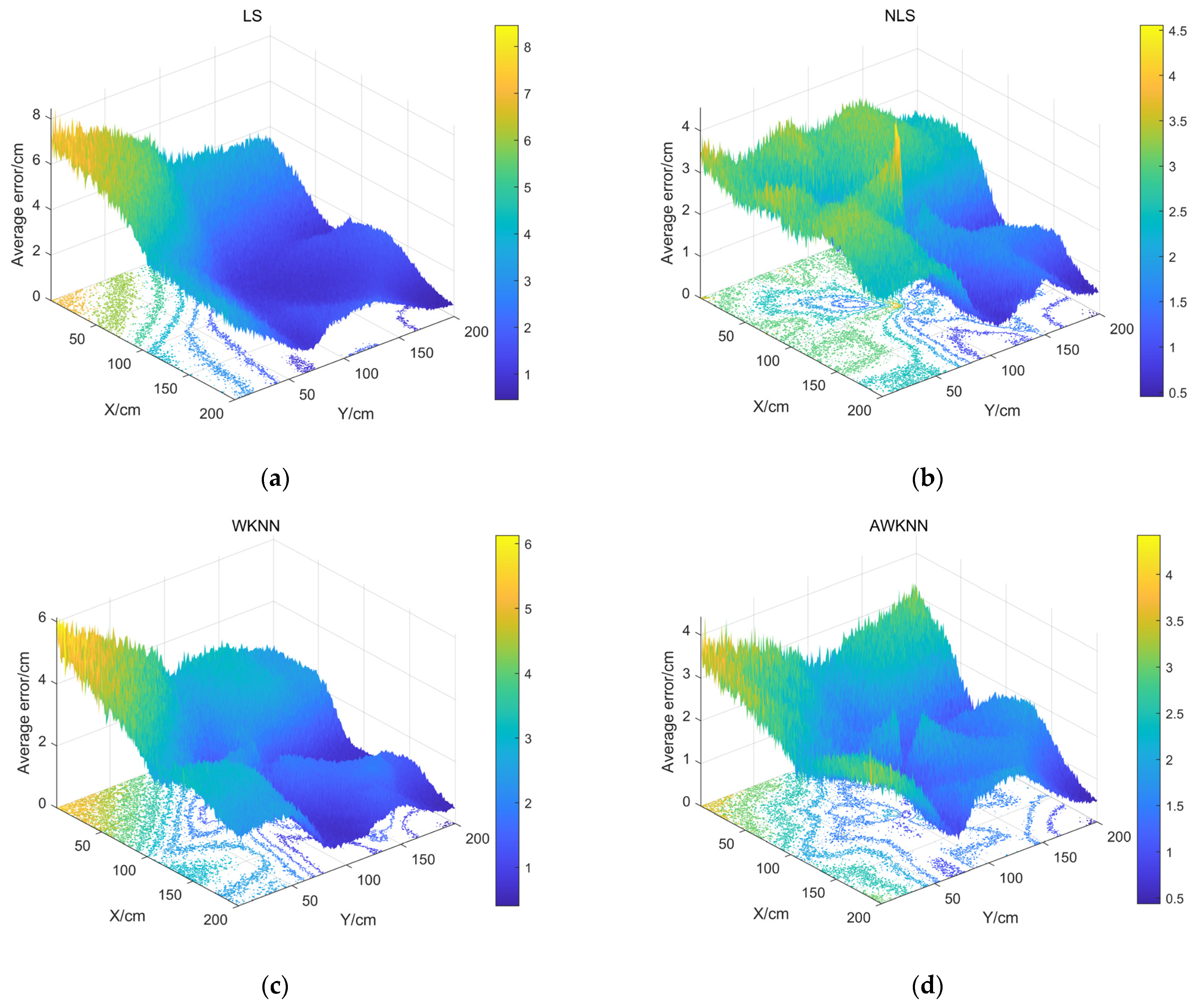
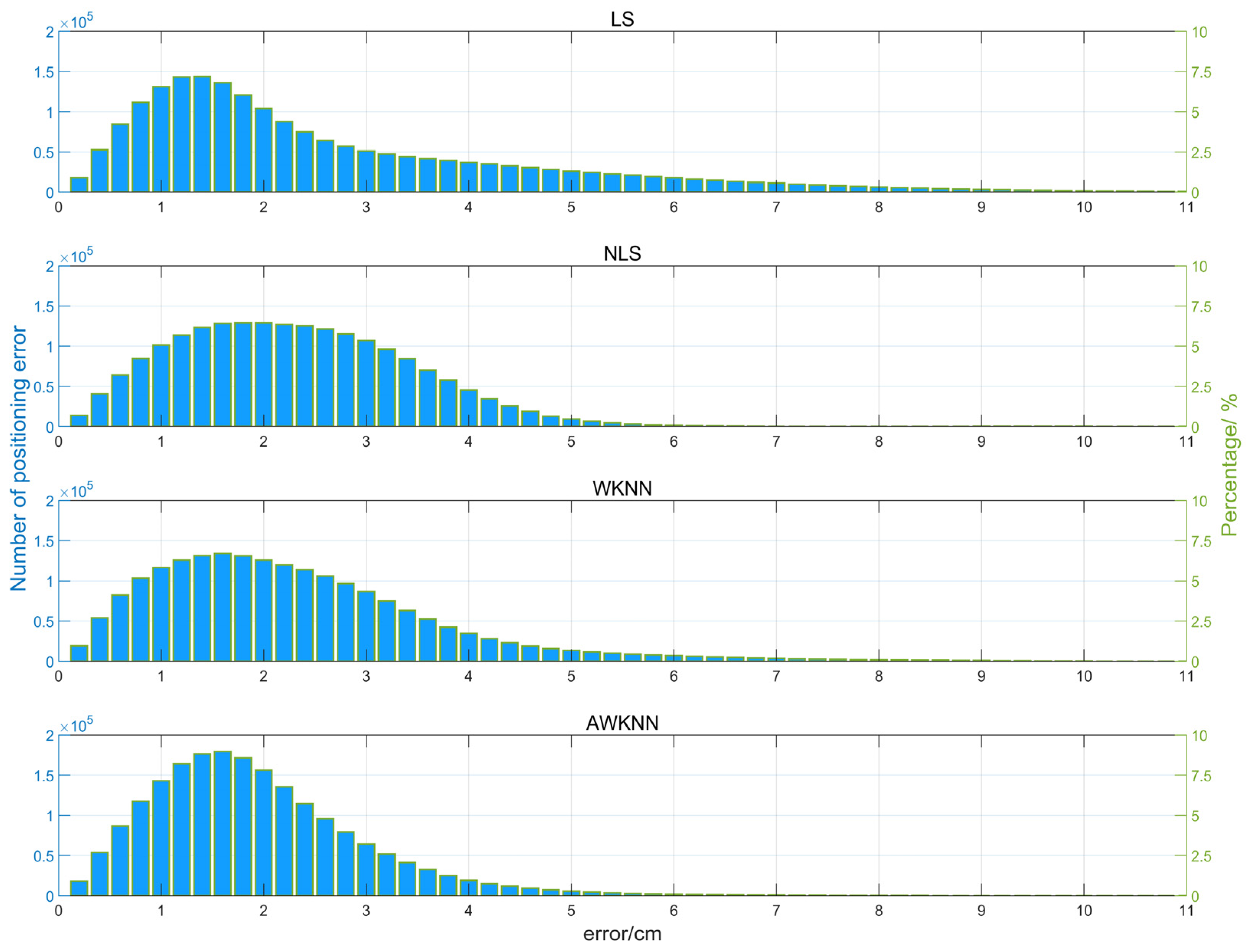
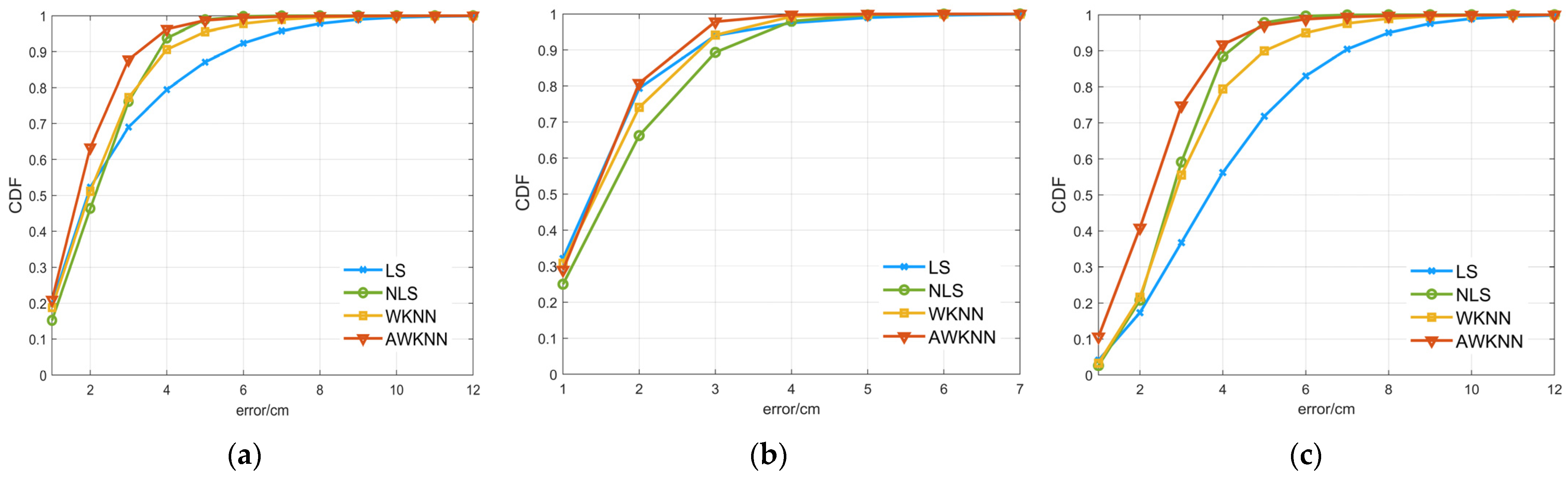
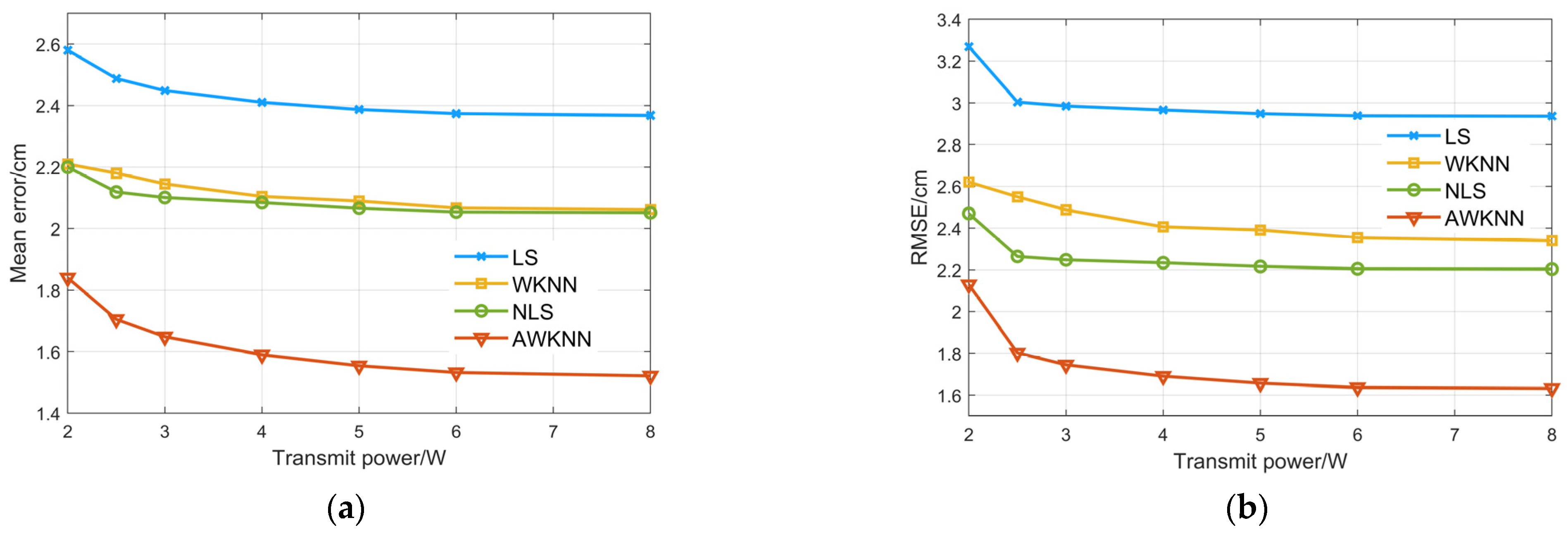
4. Results and Discussion

4.1. Simulation Setup

In this study, the performance of the AWKNN algorithm was simulated and analyzed using the LED distribution scene in Figure 1. Three existing methods were selected as comparison methods, namely, the CSI-based LS localization method proposed in [14], which is abbreviated as LS; the nonlinear LS estimation in [13] combined with the CSI-based ranging, which is abbreviated as NLS; and the modified WKNN method combined with the CSI-based ranging, which is abbreviated as WKNN. In the NLS method, the number of iterations was 6, and 25 points with a spacing of 1 cm around the estimated position were selected for each iteration, arranged in a 5 × 5 square. In the WKNN method, the K-value was set to 5, and the size of the location set was set to 25, for a fair comparison. The simulation parameters are presented in

Table 1. Simulation Parameters.

	Symbol	Parameter	Value
room parameters	L × W × H	size of the simulation environment	4 m × 4 m × 3 m
	$\rho$	reflectance factor of the wall	0.33
	$A_{wall}$	reflective area of each reflection point	1 cm2
transmitter parameters	N	number of LEDs	4
	m	order of Lambertian emission	2.6
	$P_t$	LED transmit power	2 W
receiver parameters	$A_{PD}$	surface area of the PD	1 cm2
	$\gamma$	PD’s responsivity	0.5 A/W
	${\theta }_{FOV}$	PD’s FOV semi-angle	80°
	$T_s(\theta )$	optical filter gain	1
	$g(\theta )$	concentrator gain	1
	$I_2$	noise bandwidth factor	0.562
	$I_3$	noise bandwidth factor	0.0868
	$I_{bg}$	background current	5100 μA
	$T_K$	circuit absolute temperature	295 K
	G	open-loop voltage gain	10
	$\eta$	fixed capacitance per unit area	112 pF/cm2
	$\Gamma$	FET channel noise factor	1.5
	$g_m$	FET transconductance	30 mS
system parameters	B	system bandwidth	125 MHz
	$N_g$	length of CP	16
	$N_T$	length of training symbol	512
	$N1$	number of pilot symbol	128
	$N_P$	length of pilot symbol	32
	$T_s$	sampling interval of the receiver signal	4 ns
	M	size of the position set in the NLS and WKNN algorithms	25
	T	number of iterations in the NLS algorithm	6
	K	number of nearest neighbors in the WKNN algorithm	5

. Considering that the LED positions in the simulation scene were symmetrical, the area selected for this simulation was 2 m × 2 m, accounting for one-quarter of the entire room. The ground was divided into many 1 cm × 1 cm grids, and the PD measured the positioning error 50 times at each grid intersection to evaluate the performance of the positioning method.

4.2. Performance Evaluation

The positioning accuracy was observed through the mean error and the root mean square error (RMSE) of the position estimation, where the RMSE is defined as

$$\mathrm{RMSE}=\sqrt{\frac{1}{N_S}{\displaystyle \sum _{m=1}^{N_S}\left[{(x_m-{\widehat{x}}_m)}^2+{(y_m-{\widehat{y}}_m)}^2\right]}},$$

(25)

where $N_S$ is the number of locations in the simulation, $(x,y)$ represents the actual horizontal coordinates of the PD, and $(\widehat{x},\widehat{y})$ denotes the estimated horizontal coordinates of the PD.

The two-dimensional distribution of the positioning errors of different methods is shown in Figure 3, where each error in the figure was the average of 50 measurements of the positioning accuracy. From the error distribution in Figure 3, it can be concluded that the positioning accuracy of all the positioning methods in the corners of the room was poor owing to the impact of the multipath reflection. This was because these positions were the farthest from all the LEDs and were most affected by the reflection path. Near the central region, the greater the optical power contribution from the LOS path, the more precise the distance estimated based on the CSI, and the lower the positioning error. Compared with the LS, WKNN, and NLS, the AWKNN had higher localization accuracy in the whole room.

The histograms of the positioning errors of different methods are demonstrated in Figure 4, which reflects the dispersion of the positioning errors. The vertical axes on the left and right in the figure represent the number of positioning errors and the corresponding proportion, respectively. It can be seen from Figure 4 that the LS’s error distribution was dispersed with a lengthy tail of large errors. The error greater than 8 cm accounted for 2.19%, which echoed the result of the LS algorithm shown in Figure 3 and was mainly caused by the error in the corner of the room. The WKNN’s error distribution was likewise dispersed with a lengthy tail, with errors larger than 6 cm accounting for 2.21% of the total. Compared to the LS and the WKNN, the NLS had a concentrated error distribution, with 1.1% of the positioning errors exceeding 5 cm. In contrast, the error distribution of the AWKNN had a shorter tail and was more concentrated in the case of small errors. In total, 63.32% of the positioning errors were less than 2 cm, with the majority being centered around 1.6 cm. This demonstrated that by adaptively selecting the weights, the proposed method effectively reduced the large positioning errors and made the positioning errors cluster at a lower level.

Figure 5 demonstrates the cumulative distribution function (CDF) curves of the positioning errors of the different methods. The CDF results revealed that in the whole room, under the condition of CDF = 95%, the localization error of the AWKNN was 3.95 cm, while that of the WKNN, NLS, and LS was 4.83 cm, 4.13 cm, and 6.73 cm, respectively. It can be seen from the CDF curve that the positioning accuracy of the AWKNN method was better than that of the three comparison methods, whether in the entire room, the edge area, or the center area. Especially in the edge area, the proposed method achieved larger performance gains, which demonstrated its higher robustness. This is all due to the proposed method using the direct path distance estimated by the CSI to adaptively adjust the K-value and weight to cope with the nonlinear errors in localization.

The positioning performance comparison of different methods is depicted in

Table 2. Comparison of the positioning performance of the different methods.

Positioning Error		LS	WKNN	NLS	AWKNN
Entire room	Mean/cm	2.58	2.21	2.20	1.84
	RMS/cm	3.27	2.62	2.47	2.13
Center area	Mean/cm	1.48	1.52	1.72	1.43
	RMS/cm	1.75	1.74	1.96	1.59
Edge area	Mean/cm	3.99	3.09	2.82	2.37
	RMS/cm	4.53	3.43	2.99	2.67

. For the entire room, the average positioning error of the AWKNN achieved 1.84 cm, and the RMSE was 2.13 cm. Compared with the LS, the AWKNN reduced the positioning mean error and the RMSE by 29% and 35%, respectively. Similarly, a reduction of about 17% and 19% in terms of mean error and the RMSE was achieved compared to the WKNN. In the edge region, the mean error and the RMSE of the AWKNN were 2.37 cm and 2.67 cm, respectively. The average localization accuracy of the AWKNN was improved by 41% and 16% over the LS and NLS, respectively. Compared with the NLS, the mean error and the RMSE of the AWKNN in the center area were decreased by about 17% and 19%, respectively. It can be observed that the proposed method outperformed the contrasting methods in all regions, which demonstrated its ability to achieve a high-precision position estimation in complex indoor multipath environments.

Next, the influence of the selection of the K-value on the positioning accuracy was analyzed. The simulation results of the positioning performance under different K-values are shown in Figure 6. It can be observed from Figure 6 that the average positioning accuracy improved with the increase in the value of K and reached the optimum when K = 2. When the value of K further increased, the performance began to decline. There were obvious differences in the positioning accuracy of the different K-values. The proposed AWKNN outperformed the WKNN using different K-values, which verified the effectiveness of the proposed algorithm for adaptively determining the K-value and weights.

To show the effect of the SNR on the positioning accuracy, we analyzed the average error and the RMSE of the positioning by varying the transmit power of the LED. Under different transmit power conditions, the positioning accuracy of the different methods is shown in Figure 7. The positioning error of all methods decreased rapidly with the increase in the LED’s transmit power and then decreased slowly until reaching a plateau. This is because increasing the transmit power of the LED can improve the SNR and reduce the influence of the channel noise on the channel estimation. However, in the DCO-OFDM system, to ensure that the LED works within the linear range, the positioning signal needs to be clipped at the transmitter, thus introducing a clipping error [14], which cannot be improved by increasing the SNR. In addition, in the CSI-based ranging method [14], a key step is to estimate the number of channel paths, which also introduces path number estimation errors. In the next step, we investigate the impact of different O-OFDM modulation schemes on the ranging and positioning accuracy to achieve high-precision positioning.

To fully analyze the performance of the proposed method, we next evaluated the time complexity of the different algorithms. As the time complexity of the multiplication and inversion of the matrices of size $m\times m$ is $\mathrm{O}(m^3)$, it can be concluded that the time complexity of the LS algorithm using Equation (14) was $\mathrm{O}(6(N-1)+2^3)$.

The time complexity of the AWKNN algorithm was obtained through the following analysis. In step 1 of the AWKNN algorithm, the position set was obtained by cyclic subtraction of the LS method. Hence, the time complexity of this process was $\mathrm{O}(N\cdot (6(N-1)+2^3))$. The input to the calculation of the distance difference was N + 1 distance vector of length N; so, the time complexity of steps 2 and 3 was $\mathrm{O}(N\cdot (N+1))$. In step 4, the input to the calculation of the weight vector in Equation (18) was a vector of length K; so, it had a time complexity of $\mathrm{O}(K)$. Similarly, the time complexity of calculating Equations (20) and (21) was both $\mathrm{O}(N\cdot K)$. The time complexity of finding the minimum from K elements in Equation (22) was $\mathrm{O}(K)$. The time complexity of the K-th iteration in step 4 was $\mathrm{O}(2K\cdot (N+1))$. Hence, the time complexity of step 4 was $\mathrm{O}(2(N+1)\cdot K_{\max }\cdot (K_{\max }+1)/2)=\mathrm{O}({(N+1)}^2\cdot (N+2))$. Since the number of weights $K^{\prime }$ in Equation (24) was uncertain, the maximum time complexity considered here was $\mathrm{O}(K_{\max })=\mathrm{O}(N+1)$. Overall, the AWKNN algorithm had a time complexity of $\mathrm{O}({(N+1)}^2\cdot (N+3)+N\cdot (6(N-1)+2^3))$. For the NLS algorithm and WKNN algorithm, the time complexities were $\mathrm{O}(6(N-1)+2^3+T\cdot M\cdot (N+1))$ and $\mathrm{O}(6(N-1)+2^3+M\cdot (N+K)+2K)$, respectively.

Table 3. Time complexity comparison.

Method	Time Complexity
LS	$\mathrm{O}(6(N-1)+2^3)$
WKNN	$\mathrm{O}(6(N-1)+2^3+M\cdot (N+K)+2K)$
NLS	$\mathrm{O}(6(N-1)+2^3+T\cdot M\cdot (N+1))$
AWKNN	$\mathrm{O}({(N+1)}^2\cdot (N+3)+N\cdot (6(N-1)+2^3))$

shows the time complexity comparison of the different methods. It can be observed that with an increase in the number of LEDs, the time complexity of the LS algorithm, WKNN algorithm, and NLS algorithm all rose linearly, while the proposed AWKNN algorithm increased rapidly. Under the parameters set as shown in Table 1, the time complexity of the LS algorithm was the lowest, followed by the time complexity of the WKNN and AWKNN algorithms, and the NLS algorithm had the highest time complexity. The proposed method had the highest complexity when the number of LEDs exceeded 8. Considering that in practical application scenarios, the density of the LED arrangement and the number of LED signals received by the PD at a specific location are limited, the time complexity of the proposed methods will not be seriously affected. Moreover, considering that the current hardware level has been greatly improved, and the computing resources are sufficient to meet the needs of the algorithm, the increase in the time complexity is acceptable.

5. Conclusions

To optimize the positioning accuracy in complex environments with multipath reflections, this work presented an AWKNN trilateration positioning algorithm fused with CSI. This method combined the WKNN and CSI-based ranging to achieve the adaptive determination of the K-value and weight according to the environmental changes, effectively reducing the positioning errors without data acquisition and training. The simulation results highlighted that the average localization accuracy of the AWKNN algorithm reached about 1.84 cm, which was increased by 29%, 16%, and 17% over the CSI-based LS method, CSI-based NLS method, and CSI-based WKNN method, respectively. The results revealed that this method achieved excellent localization accuracy and robustness in complex scenes. In our future work, we will build a prototype and verify the performance of the proposed positioning method through experiments. In addition, we will further study the impact of different O-OFDM modulation schemes on the positioning accuracy to achieve high-precision positioning with a high modulation bandwidth.

References

- Farahsari, P.S.; Farahzadi, A.; Rezazadeh, J.; Bagheri, A. A Survey on Indoor Positioning Systems for IoT-Based Applications. IEEE Internet Things J. 2022, 9, 7680–7699. [Google Scholar] [CrossRef]
- Guo, X.; Ansari, N.; Hu, F.; Shao, Y.; Elikplim, N.R.; Li, L. A Survey on Fusion-Based Indoor Positioning. IEEE Commun. Surv. Tutor. 2020, 22, 566–594. [Google Scholar] [CrossRef]
- Zafari, F.; Gkelias, A.; Leung, K.K. A survey of indoor localization systems and technologies. IEEE Commun. Surv. Tutor. 2019, 21, 2568–2599. [Google Scholar] [CrossRef]
- Matheus, L.E.M.; Vieira, A.B.; Vieira, L.F.M.; Vieira, M.A.M.; Gnawali, O. Visible Light Communication: Concepts, Applications and Challenges. IEEE Commun. Surv. Tutor. 2019, 21, 3204–3237. [Google Scholar] [CrossRef]
- Huang, N.; Gong, C.; Luo, J.; Xu, Z. Design and Demonstration of Robust Visible Light Positioning Based on Received Signal Strength. J. Light. Technol. 2020, 38, 5695–5707. [Google Scholar] [CrossRef]
- Martínez-Ciro, R.A.; López-Giraldo, F.E.; Luna-Rivera, J.M.; Ramírez-Aguilera, A.M. An Indoor Visible Light Positioning System for Multi-Cell Networks. Photonics 2022, 9, 146. [Google Scholar] [CrossRef]
- Steendam, H. A 3-D positioning algorithm for AOA-based VLP with an aperture-based receiver. IEEE J. Sel. Areas Commun. 2018, 36, 23–33. [Google Scholar] [CrossRef]
- Zhao, H.; Wang, J. A Novel Three-Dimensional Algorithm Based on Practical Indoor Visible Light Positioning. IEEE Photonics J. 2019, 11, 6101308. [Google Scholar] [CrossRef]
- Du, P.; Zhang, S.; Chen, C.; Alphones, A.; Zhong, W.-D. Demonstration of a Low-Complexity Indoor Visible Light Positioning System Using an Enhanced TDOA Scheme. IEEE Photonics J. 2018, 10, 7905110. [Google Scholar] [CrossRef]
- Meng, X.; Jia, C.; Cai, C.; He, F.; Wang, Q. Indoor High-Precision 3D Positioning System Based on Visible-Light Communication Using Improved Whale Optimization Algorithm. Photonics 2022, 9, 93. [Google Scholar] [CrossRef]
- Bai, L.; Yang, Y.; Feng, C.; Guo, C. Received signal strength assisted perspective-three-point algorithm for indoor visible light positioning. Opt. Express 2020, 28, 28045–28059. [Google Scholar] [CrossRef]
- Liu, X.; Zou, D.; Huang, N.; Wang, Y. An Efficient Iterative Least Square Method for Indoor Visible Light Positioning under Shot Noise. IEEE Photonics J. 2022, 15, 7300910. [Google Scholar] [CrossRef]
- Gu, W.; Aminikashani, M.; Deng, P.; Kavehrad, M. Impact of Multipath Reflections on the Performance of Indoor Visible Light Positioning Systems. J. Light. Technol. 2016, 34, 2578–2587. [Google Scholar] [CrossRef]
- Wang, K.; Liu, Y.; Hong, Z. RSS-based visible light positioning based on channel state information. Opt. Express 2022, 30, 56. [Google Scholar] [CrossRef]
- Bakar, A.; Glass, T.; Tee, H.; Alam, F.; Legg, M. Accurate visible light positioning using multiple-photodiode receiver and machine learning. IEEE Trans. Instrum. Meas. 2021, 70, 7500812. [Google Scholar] [CrossRef]
- Tran, H.Q.; Ha, C. High Precision Weighted Optimum K-Nearest Neighbors Algorithm for Indoor Visible Light Positioning Applications. IEEE Access 2020, 8, 114597–114607. [Google Scholar] [CrossRef]
- Xu, S.; Chen, C.C.; Wu, Y.; Wang, X.; Wei, F. Adaptive Residual Weighted K-Nearest Neighbor Fingerprint Positioning Algorithm Based on Visible Light Communication. Sensors 2020, 20, 4432. [Google Scholar] [CrossRef]
- Lin, D.C.; Chow, C.W.; Peng, C.W.; Hung, T.Y.; Chang, Y.H.; Song, S.H.; Lin, Y.S.; Liu, Y.; Lin, K.H. Positioning unit cell model duplication with residual concatenation neural network (RCNN) and transfer learning for visible light positioning (VLP). J. Light. Technol. 2021, 39, 6366–6372. [Google Scholar] [CrossRef]
- Chen, H.; Han, W.; Wang, J.; Lu, H.; Chen, D.; Jin, J.; Feng, L. High accuracy indoor visible light positioning using a long short term memory-fully connected network based algorithm. Opt. Express 2021, 29, 41109–41120. [Google Scholar] [CrossRef]
- Hsu, L.; Tsai, D.; Chen, H.M.; Chang, Y.; Liu, Y.; Chow, C.; Song, S.; Yeh, C. Using Received-Signal-Strength (RSS) Pre-Processing and Convolutional Neural Network (CNN) to Enhance Position Accuracy in Visible Light Positioning (VLP). In Proceedings of the Optical Fiber Communication Conference (OFC) 2022, San Diego, CA, USA, 6–10 March 2022. [Google Scholar]
- Cao, Z.; Cheng, M.; Yang, Q.; Tang, M.; Liu, D.; Deng, L. Experimental investigation of environmental interference mitigation and blocked LEDs using a memory-artificial neural network in 3D indoor visible light positioning systems. Opt. Express 2021, 29, 33937–33953. [Google Scholar] [CrossRef]
- Lin, X.; Zhang, L. Intelligent and Practical Deep Learning Aided Positioning Design for Visible Light Communication Receivers. IEEE Commun. Lett. 2020, 3, 577–580. [Google Scholar] [CrossRef]
- Liu, R.; Liang, Z.; Yang, K.; Li, W. Machine Learning Based Visible Light Indoor Positioning With Single-LED and Single Rotatable Photo Detector. IEEE Photonics J. 2022, 14, 7322511. [Google Scholar] [CrossRef]
- Wang, K.; Liu, Y.; Hong, Z. A Novel Timing Synchronization Method for DCO-OFDM-Based VLC Systems. IEEE Photon. J. 2021, 13, 7300709. [Google Scholar] [CrossRef]
- Wang, K. Simulation Results of CSI-Based AWKNN; FigShare. Available online: https://figshare.com/articles/dataset/Simulation_Results_of_CSI-Based_AWKNN/22276759 (accessed on 21 December 2022).