Suppression for Phase Error of Fringe Projection Profilometry Using Outlier-Detection Model: Development of an Easy and Accurate Method for Measurement

Abstract

Fringe projection is an important technology in three-dimensional measurement and target recognition. The measurement accuracy depends heavily on the calibration of the absolute phase and projector pixels. An easy-to-implement calibration method based on the Random Sample Consensus (RANSAC) algorithm is proposed to exterminate the phase error data and elevate the measurement accuracy in a fringe projection system. The reconstruction experiments of a double-sphere standard demonstrate that the uncertainties in radius and sphere-distance measurement are reduced to one thousandth of the measured value or even less, and the standard deviation in multiple measurements is restricted to within 50 μm. The measurement accuracy provided by the proposed RANSAC method can be improved by up to 44% compared with that provided by traditional least squared method (LSM). The proposed calibration method is easy and simple to implement, and it does not need additional hardware, but rather a calibration board.

1. Introduction

Fringe projection is a time-efficient and non-contact technique in 3D measurements. Compared with the traditional coordinate measurement machine, fringe projection has some major advantages, such as the nondestructive shape encoding of most materials by using the structured visible or non-visible light patterns in a point cloud map with a huge amount of data in one measurement. These overwhelming merits bring about great application prospects. After decades of development, fringe projection profilometry has steadily expanded its working scenario and applications, such as in situ measurement in industrial production and processing, rapid feature recognition, and human–machine interactive scenes like augmented reality (AR) or mixed reality (MR). In recent years, structured light systems have been developed rapidly. One of these branches, reflectometry, is commonly utilized for measuring the surface slopes of highly reflective surfaces based on the geometry of the fringe reflection. The Software Configurable Optical Test System (SCOTS) [1], which evolved from reflectometry, plays a dominant role in accurately and rapidly measuring large and highly aspherical shapes such as solar collectors and primary mirrors for astronomical telescopes [2]. As an efficient, noncontact measurement method, the SCOTS technique is more suitable for measuring specular reflective surfaces, while fringe projection techniques are more suitable for measuring diffuse reflective surfaces. Similar to fringe projection techniques, the SCOTS technique also relies on the calibration accuracy of systems, and a careful calibration can effectively improve the measuring accuracy [3]. Therefore, researchers conducted extensive research on improving measuring accuracy, and various novel coding strategies were proposed, such as phase-shifting [4,5], Fourier transform [6,7], color-indexing [8], temporal-spatial coding [9,10] methods, as well as some phase unwrapping strategies, including gray-code [11], multi-frequency heterodyne [12] and so on. However, as measurement technologies, the accuracy of these strategies is a vital assessment index of their performance. Many researchers have focused on reducing the source errors of uncertainty and elevating reconstruction accuracy and stability while making a system easier to calibrate. From the perspective of measurement accuracy, there have been theories proving that distortion of the camera and projector lens would cause systematic errors and affect the precision of measurement results [13,14]. To eliminate this error, the intrinsic and extrinsic parameters of cameras and projectors should be finely calibrated, and the image distortion should be compensated [15,16]. Some other research works contribute to the accuracy improvement through gamma correction [17,18,19].

From the perspective of system calibration, two types of methods are commonly utilized. Some studies utilizing polynomial [20], least-square [21] or Gaussian Process regression [22] methods to implement the three-dimensional (3D) calibration process in a fringe projection system. Among these methods, the assistance of high-precision displacement positioning platforms is essential, which makes the calibration process costly. Zhang et al. [23] proposed a general and widely recognized 3D calibration method for a fringe projection system, which directly finds the relationship between the height value and the phase value. The calibration board can be placed randomly in the measurement volume, but it needs at least 13 pictures at each position. On the other hand, An et al. [24] proposed another calibration method for monocular phase-shifting structured light profilometry and explained the 3D reconstruction theory as well as the effect of geometric constraints. This provided a preliminary theoretical reference for analyzing the accuracy of a fringe projection measurement system [25]. Compared to the method that directly derives the relation between height and phase, the difficulty of calibration is significantly reduced, as no displacement of the positioning platform is involved. However, its reconstruction accuracy depends heavily on the accuracy of the relationship between the phase value and the projector pixel position.

Literature reviews shows that, in a geometric constraint-based monocular phase-shifting fringe projection system, the relationship between the coding phase and the projection position has rarely been discussed, while the calibration process is vital for reconstruction precision. In this paper, the phase errors in calibrating the absolute phase and projector pixel relation are investigated. A calibration method based on random sample consensus (RANSAC) is proposed to eliminate the error data in a phase map. The experiments demonstrate that the well-calibrated system based on the proposed method can achieve millesimal uncertainty, or even less. The accuracy as well as the stability of the system are significantly improved compared to those provided by a traditional method. The proposed method is easy to implement and suitable for most monocular phase-shifting fringe projection systems generally.

2. Principles

In this research, we employ the four-step phase-shifting method to calculate the wrapped phase, and the multi-frequency heterodyne phase unwrapping technique to calculate the unwrapped phase (or absolute phase). In this section, the 3D reconstruction principle of the phase-shifting fringe projection profilometry will be explained step by step. Figure 1 demonstrates the main procedure of the profilometry, which generally includes the fringe process and system calibration. In the fringe process, fringe projection and receiving, wrapped phase calculation and phase unwrapping are performed. In system calibration, camera intrinsic calibration, projector extrinsic calibration relative to the camera and correction of the projector’s gamma effect are performed.

2.1. Phase Calculation

In the four-step phase-shifting method, a group of sinusoidal fringe pictures with a phase step of $\mathsf{\pi }/2$ are projected, which can be described in Equation (1),

$$\left\{\begin{array}{c}{I}_1\left(x,y\right)=A\left(x,y\right)+B(x,y)\cos (\phi \left(x,y\right)+\frac{\mathsf{\pi }}{2})\\ I_2\left(x,y\right)=A\left(x,y\right)+B(x,y)\cos (\phi \left(x,y\right)+\mathsf{\pi })\\ I_3\left(x,y\right)=A\left(x,y\right)+B(x,y)\cos (\phi \left(x,y\right)+\frac{3\mathsf{\pi }}{2})\\ I_4\left(x,y\right)=A\left(x,y\right)+B(x,y)\cos (\phi \left(x,y\right)+2\mathsf{\pi })\end{array}\right.$$

(1)

where I₁~I₄ represent the four patterns with different initial phases. A(x, y) is the background intensities, and B(x, y) is the modulated intensities. With I₁~I₄, the wrapped spatial phase distribution $\phi (x,y)$ can be derived as follows,

$$\phi \left(x,y\right)=\mathrm{a}\mathrm{r}\mathrm{c}\mathrm{t}\mathrm{a}\mathrm{n}\left(\left(I_3-I_1\right)/\left(I_4-I_2\right)\right)$$

(2)

Then, the phase unwrapping is essential. The multi-frequency heterodyne method provides the highest reliability of the absolute phase among the temporal phase unwrapping methods [26,27], among which the absolute phase value of each pixel is unrelated to adjacent ones. It is widely implemented in static objects with large superficial discontinuities and separations when the sampling time cost is acceptable. According to the optimal heterodyne frequency selection theory [27], frequency selection according to Equation (3) can provide the expansion range that maximizes the continuous phase.

$$N_{fi}=N_{f0}-{(N_{f0})}^{\frac{i-1}{n-1}},fori=1,2,\dots ,n-1$$

(3)

where $N_{f0}$ is the fringe period number of selected maximum frequency, and $N_{fi}$ is the fringe period number of the i-th fringe (i is not equal to 0). n expresses the group number of phase shifting number. For example, when n = 3, we set $N_{f0}$ as 64, then $N_{f1}$ is 64 − 1, that is, 63, and $N_{f2}$ is 64 − 8, that is, 56. For each pair of patterns with a smaller frequency $f_1$ and a larger frequency $f_2$, the heterodyne equivalent phase and equivalent wavelength are

$$\left\{\begin{array}{c}{\phi }_{eq}\left(x,y\right)={\phi }_{f_1}\left(x,y\right)-{\phi }_{f_2}\left(x,y\right)\\ {\lambda }_{eq}={\lambda }_1{\lambda }_2/\left({\lambda }_2-{\lambda }_1\right)\end{array}\right.$$

(4)

where ${\phi }_{f_1}\left(x,y\right)$ and ${\phi }_{f_2}\left(x,y\right)$ represent the phase distribution of frequency $f_1$ (wavelength ${\lambda }_1$) and $f_2$ (wavelength ${\lambda }_2$), respectively. ${\phi }_{eq}\left(x,y\right)$ is the heterodyne equivalent phase distribution and ${\lambda }_{eq}$ is the equivalent wavelength. Then, the phase step distribution $K\left(x,y\right)$ of each pixel can be determined as follows:

$$K\left(x,y\right)=\mathrm{r}\mathrm{o}\mathrm{u}\mathrm{n}\mathrm{d}\left[\frac{({\lambda }_{eq}/{\lambda }_2){\phi }_{eq}(x,y)-{\phi }_2(x,y)}{2\mathsf{\pi }}\right]$$

(5)

In this paper, the heterodyne phase pairs ${\phi }_{64}$ − ${\phi }_{56}$ and ${\phi }_{63}$ − ${\phi }_{56}$ are grouped to derive equivalent phase maps ${\phi }_{eq1}$ and ${\phi }_{eq2}$, then the final absolute phase ${\phi }_{abs}$ is derived by solving the heterodyne phase pair of ${\phi }_{eq1}$ − ${\phi }_{eq2}$.

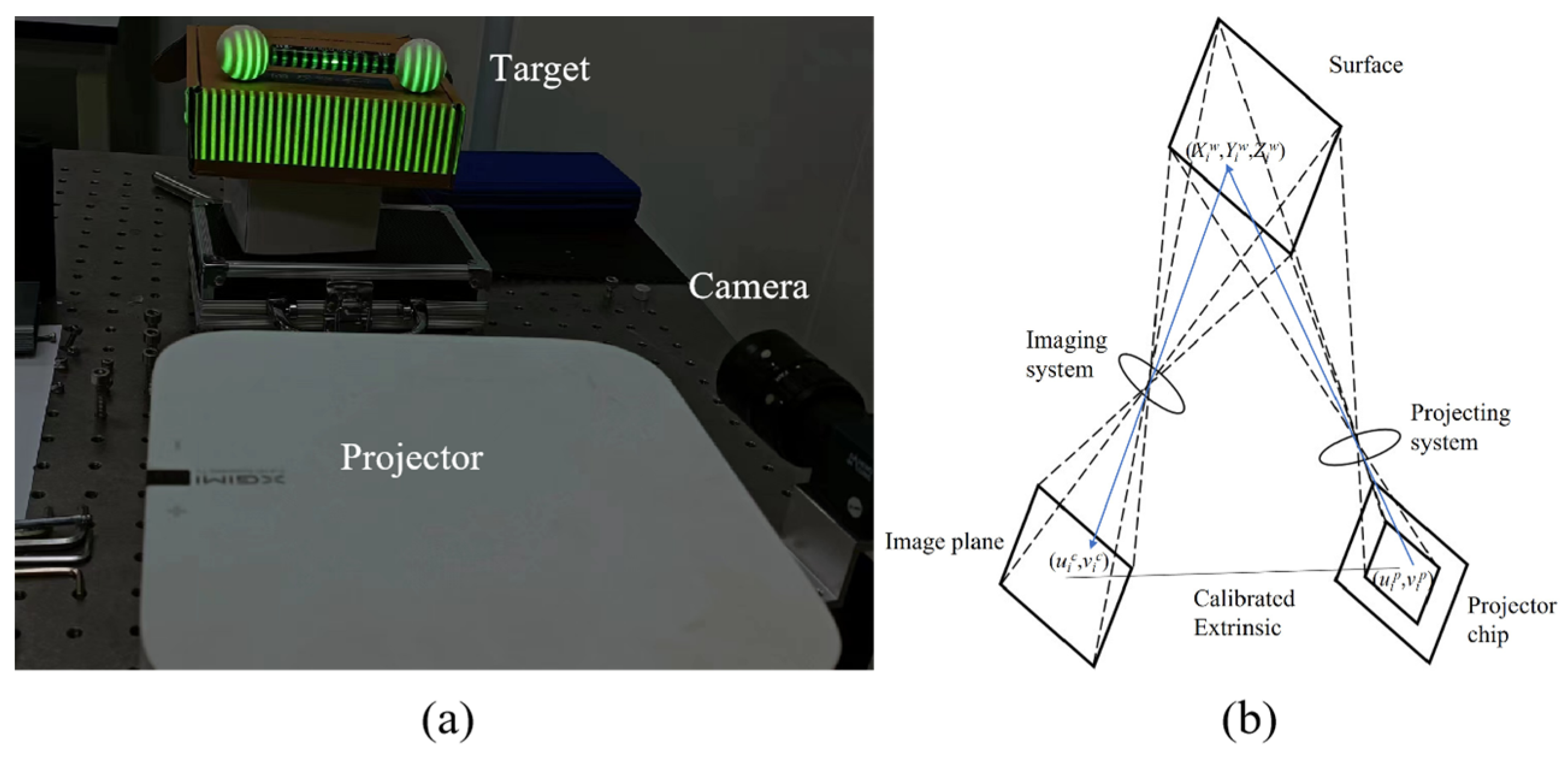
2.2. Three-Dimensional Reconstruction Model

In a common fringe projection system, the sensor is simplified as a pin-hole camera; hence, any point $P_i(X_i^W,Y_i^W,Z_i^W)$ of the world coordinate system (WCS) would be mapped to a pixel point $p_i(u_i^c,v_i^c)$ in the camera lens coordinate system by the transformation below [16],

$$\left\{\begin{array}{c}{s\left[\begin{array}{ccc}{u}_i^c& v_i^c& 1\end{array}\right]}^T={\mathrm{A}\left[\begin{array}{cc}{\mathrm{R}}_{3\times 3}& {\mathrm{T}}_{3\times 1}\\ 0_{1\times 3}& 1\end{array}\right][\begin{array}{cccc}{X}_i^w& Y_i^w& Z_i^w& 1\end{array}]}^T\\ \mathrm{A}=\left[\begin{array}{cccc}{f}_x& \gamma & u_0& 0\\ 0& f_y& v_0& 0\\ 0& 0& 0& 0\end{array}\right],\mathrm{R}=\left[\begin{array}{ccc}{r}_{11}& r_{12}& r_{13}\\ r_{21}& r_{22}& r_{23}\\ r_{31}& r_{32}& r_{33}\end{array}\right],\mathrm{T}=\left[\begin{array}{c}{t}_1\\ t_2\\ t_3\end{array}\right]\end{array}\right.$$

(6)

where A is the intrinsic matrix, [R, T] represents the extrinsic matrix which relates the world coordinate system to the camera lens coordinate system, and s is a constant scale factor. The transformation can be integrated to a matrix P [24]. As the projection can be regarded as a reverse process of imaging, the projector can be simplified as a reverse pin-hole camera as well.

$$\left\{\begin{array}{c}{s^c\left[\begin{array}{ccc}{u}_i^c& v_i^c& 1\end{array}\right]}^T={{\mathrm{P}}^c\left[\begin{array}{cccc}{X}_i^w& Y_i^w& Z_i^w& 1\end{array}\right]}^T,\\ {s^p\left[\begin{array}{ccc}{u}_i^p& v_i^p& 1\end{array}\right]}^T={{\mathrm{P}}^p\left[\begin{array}{cccc}{X}_i^w& Y_i^w& Z_i^w& 1\end{array}\right]}^T\end{array}\right.$$

(7)

where the upper label c represents the camera, while p represents the projector. ${\mathrm{P}}^c$ is the transformation matrix of camera, and ${\mathrm{P}}^p$ is the matrix of projector. Equation (7) illustrates the transformations from a point $(X_i^W,Y_i^W,Z_i^W)$ of the profile surface to the corresponding projector pixel $(u_i^p,v_i^p)$ and the camera pixel $(u_i^c,v_i^c)$. When $u_i^c$, $v_i^c$ and $u_i^p$ for vertical fringes or $v_i^p$ or horizontal fringes are known, $(X_i^W,Y_i^W,Z_i^W)$ can be determined uniquely [24,25]. The uncertainty of measurement predominantly relies on the accuracy of $u_i^c$, $v_i^c$, and $u_i^p$ (or $v_i^p$). In phase-shifting profilometry, $u_i^c$ and $v_i^c$ are highly related to the resolution of the camera sensor chip as well as the imaging distortion of the camera, while $u_i^p$ (or $v_i^p$) is highly related to the absolute phase map. Lens distortions can be rectified during system calibration to reduce the uncertainty of $u_i^c$ and $v_i^c$ [28]. To elevate the accuracy of profilometry, the projector pixel $u_i^p$ (or $v_i^p$) must be determined accurately and precisely.

2.3. Absolute Phase to Projector Pixel Calibration

In a phase-shifting system, the projector pixel $u_i^p$ is proportional to the unwrapped phase ${\phi }_{abs}$. To establish the ${\phi }_{abs}$ − $u_i^p$ relation, Zhang et al. [25] proposed a calibration strategy which takes a sample of the average phase value at the center pixel of the projected picture to determine this relation. However, even though it is the most robust unwrapping method, the multi-frequency heterodyne approach can still entail some unwrapping jump errors of the phase [27], which makes the average phase value at only one pixel unstable and causes the uncertainty of estimation. Hence, a method to expel the errors and find a well-calibrated ${\phi }_{abs}$ − $u_i^p$ relationship is needed.

As the multi-frequency heterodyne approach guarantees a high success rate of phase unwrapping, an optimal solution supported by the majority of the correct unwrapping phases in the phase map should exist. Hence, a full-frame sampling and optimal solution fitting strategy can expel the phase errors and calibrate the system accurately. Hence, an extra set of auxiliary fringes are designed to sample the absolute phases. Each picture is lit up by one vertical line which represents a known projector column pixel coordinate, referred to as the mark pixel, and different pictures represent different mark pixels. The phase map is sampled in a full frame by taking the auxiliary fringes as masks so that the true phase value at these mark pixels can be derived. In this paper, for instance, the left limit of the camera’s FOV corresponds to the 150th pixel of the projector, and the right limit corresponds to the 1770th pixel, meaning that the range can be evenly divisible by 60. Thus, a 60-pixel interval is chosen, and a set of vertical lines at mark pixels from 150 to 1770 at an interval of 60 pixels in a full-frame picture are chosen to ensure sufficient correspondence between the phase and pixels of projector. Moreover, as it exactly corresponds to half the basic frequency of stripes, considering that the phase errors are more easily introduced into the intersection of phase steps during the unwrapping process [26], the unwrapping error can be reduced by choosing periodic fringes related to the period of the wrapping fringes, and setting sampling fringes in the middle of the wrapped phase. Next, the RANSAC fitting program is introduced to divide the sample points into the inlier group representing the correct phase and the outlier group representing the error phase and to find the optimal relationship between the actual absolute phase and the projector pixel among the inliers. Finally, the fitting result is utilized in the 3D reconstruction shown in Equation (6).

RANSAC is commonly utilized for estimating the optimal solution of a target mathematical problem iteratively from an observation dataset containing inliers and outliers [28,29]. The algorithm principle is as follows:

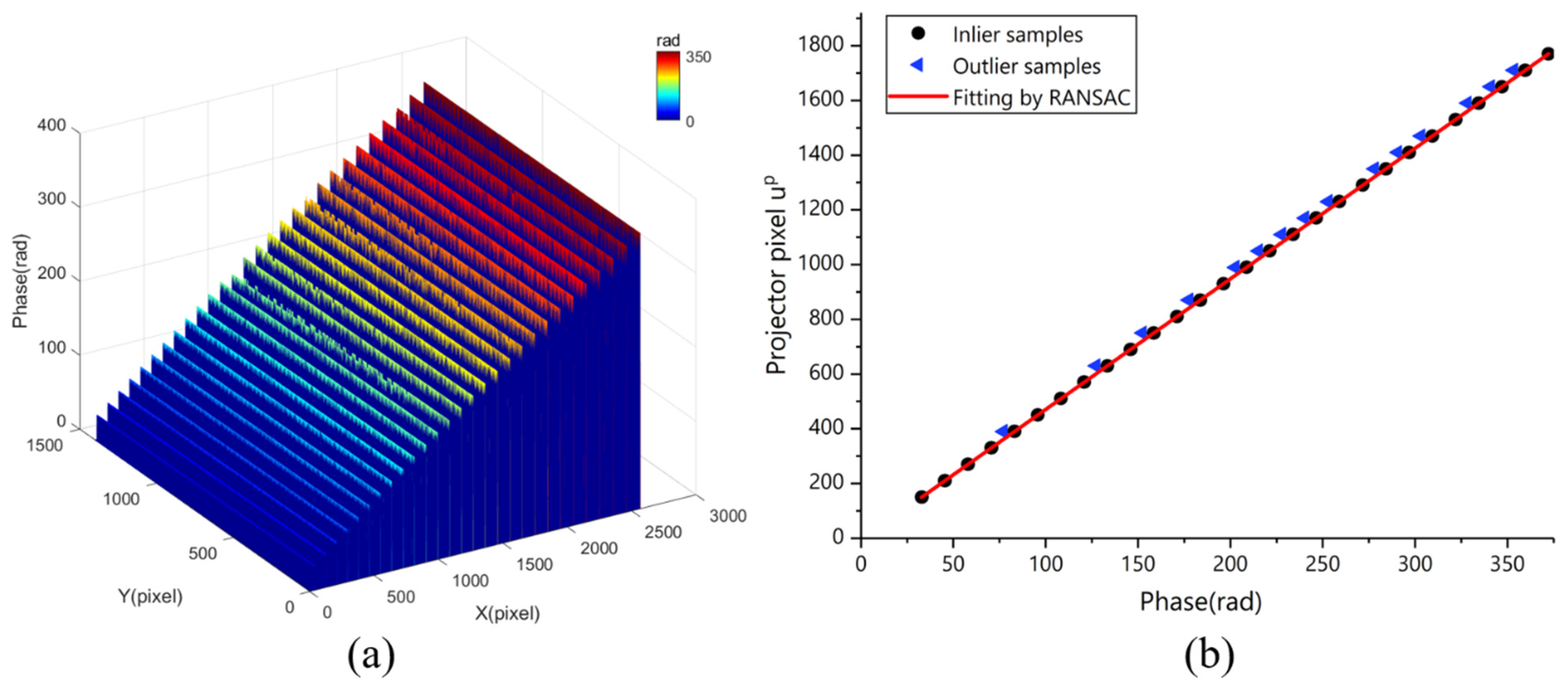
• Select the minimum dataset that can estimate the model, e.g., two points for straight line fitting,
• Use the minimum dataset to calculate the model;
• Insert all data into the model to determine the inliers, which remain within acceptable errors with the model. Meanwhile, the remaining data are outliers. Inliers follow the model well, while outliers reject it strongly.
• Compare the number of inliers between the current model and the best model previously calculated. The quality of a model is positively correlated with the number of inliers.
• Repeat steps 1–4 until the quality of the model meets the desired value (the number of inliers is greater than the desired number)

RANSAC is an uncertain algorithm, which has a certain probability to obtain a reasonable result; the more iterations, the greater the probability, which is expressed as,

$$K=\raisebox{1ex}{$\ln \left(1-P\right)$}\!\left/ \!\raisebox{-1ex}{$\ln \left(1-{\omega }^n\right)$}\right.$$

(8)

where $K$ is the number of iterations, $\omega$ is the proportion of inliers in all data, $n$ is the number of selected data, and $P$ is the probability of randomly selected points being inliers during the iteration process. The target of the algorithm is to find a model with the lowest cost function. Every time, the algorithm randomly picks a group of the lowest number of samples that can produce model parameters from the original dataset to generate a model. Then, the algorithm traverses the dataset and check if the rest of the data fit the model. This process is executed enough times to find the optimal model. Among all the fitted models, the one with the lowest cost is the optimal solution. In RANSAC algorithms, if a datum is labelled as an inlier, the cost function is assigned a value of zero, while an outlier datum causes the cost function to be assigned a value of 1. So, the output of the algorithm is the model with the most inliers. The multi-frequency heterodyne method ensures that there are enough correct phases, which means an optimal solution exists, and the jump errors are usually around 2π or greater. Therefore, an appropriate threshold can be figured out to distinguish the inliers and outliers. Based on the above discussion, the RANSAC method is suitable for the calibration of the ${\phi }_{abs}$ − $u_i^p$ relationship considering the jump errors.

3. System Calibration

3.1. System Setup

The assembled monocular structured light profilometry system is composed of a projector and an industrial camera. The digital projector is a Xgimi Z6 with a resolution of 1920 × 1080. The camera is a Daheng MER-500-14GM/C with a resolution of 2592 × 1944. The whole system was well calibrated. The “Camera Calibration Toolbox” in Matlab^® software (R2023) was adopted to calibrate the intrinsic parameters of the camera [30], and the “Camera-Projector Calibration Toolbox” was adopted to calibrate the intrinsic parameters of the projector as well as the extrinsic parameters relative to the camera [31]. The correction of camera distortion, which includes two terms of radial distortion and two terms of tangential distortion, was implemented based on the results of calibration as well. The fringe projection system built is shown in Figure 2a and the system schematic diagram with detailed measuring principles is shown in Figure 2b. For example, beam light is emitted from the pixel ($u_i^p$, $v_i^p$) and projected onto the target surface of the 3D point ($X_i^w$, $Y_i^w$, $Z_i^w$). Then, the scattered beam arrives at ($u_i^c$, $v_i^c$) of the image plane in the camera. With known $u_i^p$, the location of point ($X_i^w$, $Y_i^w$, $Z_i^w$) can be solved using the linear problem in Equation (7).

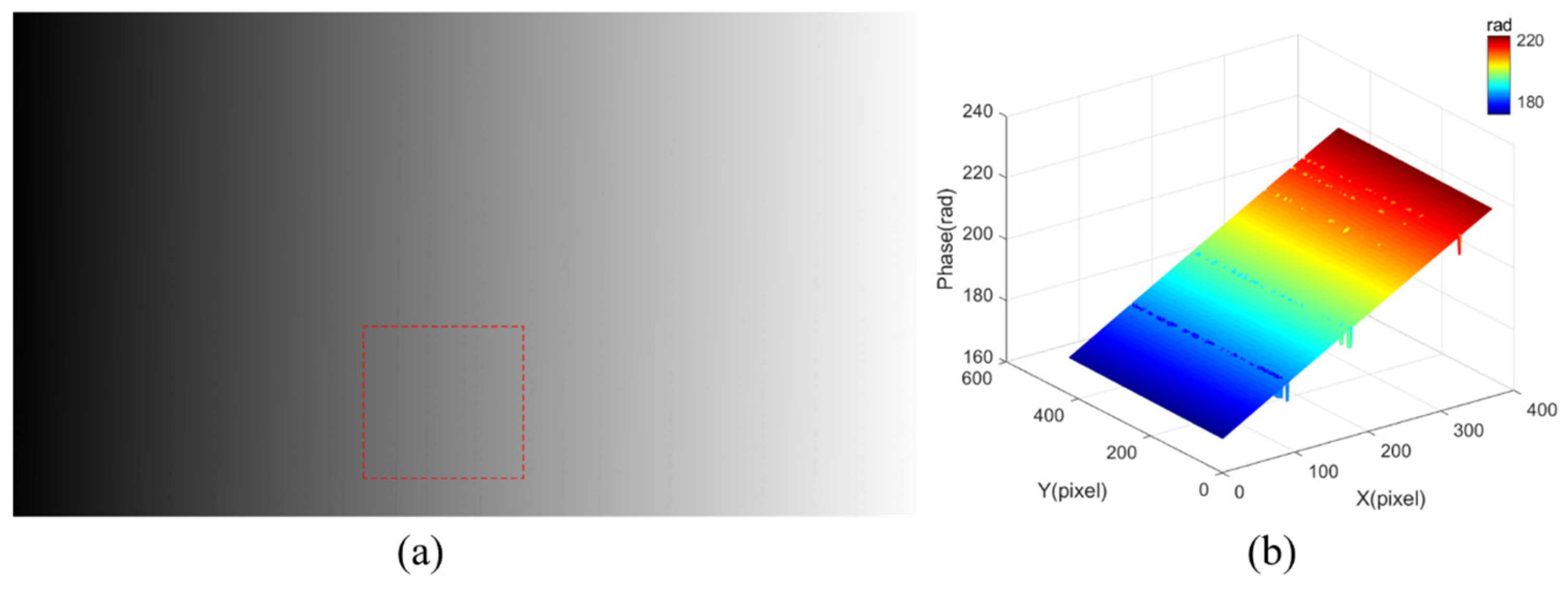
3.2. Gamma Correction

The nonlinear output characteristics of a projector are also known as the gamma effect, which could cause corrugated errors in a fringe projection system. In this experiment, an active compensation method is utilized to eliminate the effects of the gamma factor. Active compensation refers to the pre-modulation performing the annihilation of the gamma effect of the ideal fringe on a computer. The purpose is to determine the fitting expression, more specifically the $b_n$ values of the inverse function of the nonlinear output of the system in Equation (9).

$$I_{in}={\sum }_{n=0}^N{b}_n{I}_{out}^n$$

(9)

The procedure of the polynomial compensation method can be described as follows:

(1)

A series of full-frame grayscale map sets with uniformly increasing grayscale values are generated by the computer.

(2)

The projector projects the grayscale map and captures it sequentially using the camera.

(3)

The grayscale values of the captured images are calculated in turn.

(4)

Taking the actual gray value as the independent variable and the preset gray value as the dependent variable, the coefficients in Equation (9) are calculated using the fitting algorithm (such as the LMS method).

(5)

Taking Equation (9) as the inverse function of the nonlinear output of the system, the ideal sinusoidal fringe is pre-modulated, and the output at this time is the ideal sinusoidal fringe to complete the compensation.

Figure 3 demonstrates the result of actively compensating the gamma effect. The output grayscale is approximately a linear function of the input grayscale.

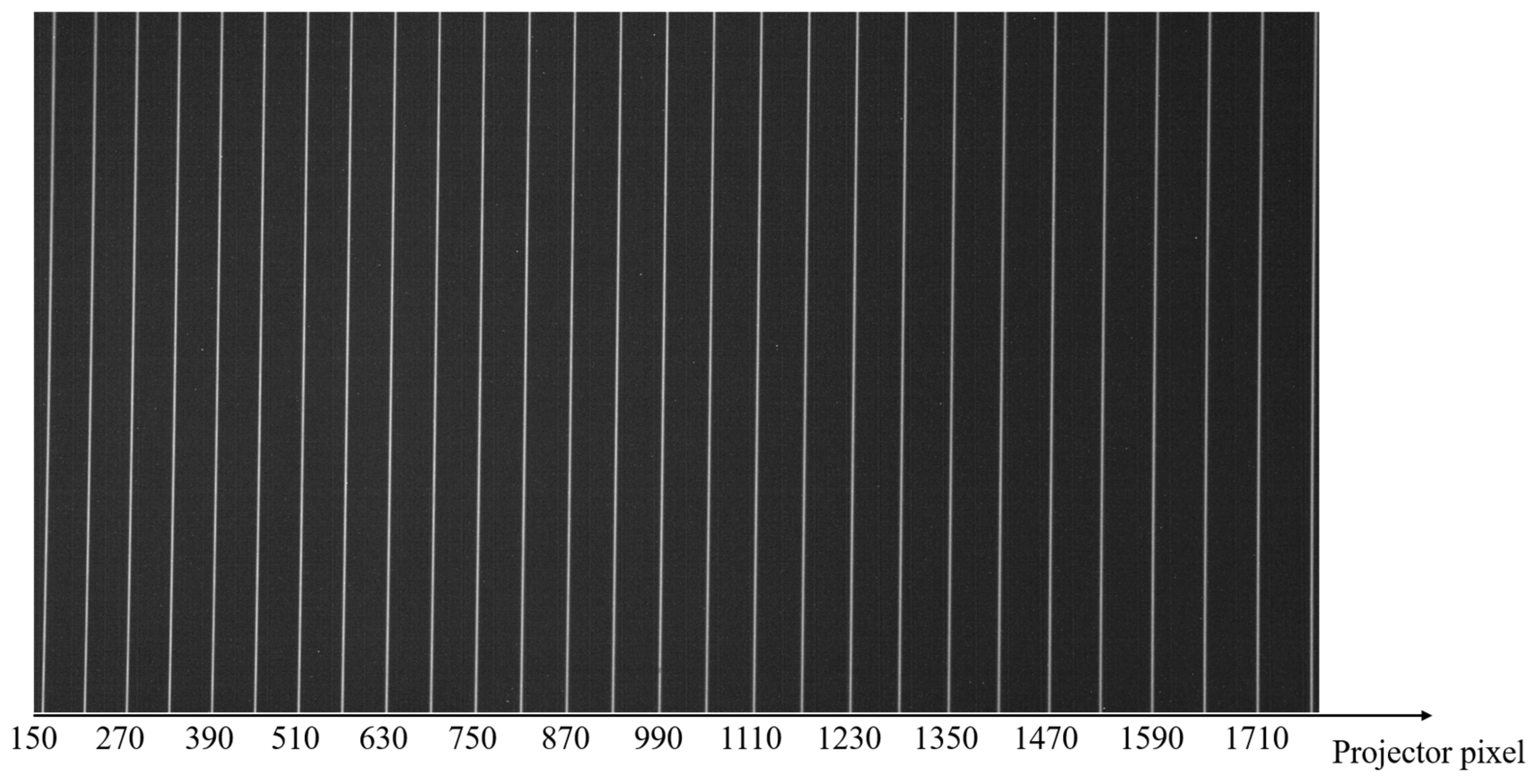
3.3. Fringe Recording

In the process of ${\phi }_{abs}$ − $u_i^p$ calibration, for the convenience of verifying the RANSAC algorithm, the phase-shifting and the auxiliary fringes were projected sequentially onto a position-fixed calibration board for guaranteeing no offset between the two groups of pictures. Figure 4a–d,f–i,k–n demonstrate the phase shifting pictures captured by the camera with fringe periods of 64, 63 and 56, respectively. Figure 4e,j,o are the modulo-2π phase maps of 64, 63 and 56, respectively. Here, it is also feasible to integrate all stripes into a single frame for projection, as long as the projector pixels at each position can be recognized.

After unwrapping, the absolute phase map is shown in Figure 5a. Figure 5b illustrates the zoomed in local phase distribution in the red box where several unwrapped error phases exist, although they accounted for a minute portion.

Then, according to the proposed method in Section 2.3, the auxiliary 28 pictures representing different pre-determined mark pixels in the projector were projected onto the same board to assist in establishing the relationship between the phase value and projector pixel. For convenience of demonstration, the 28 captured pictures were compressed into one, which is shown in Figure 6.

3.4. ${\phi }_{abs}$ − $u_i^p$ Relation Calibration by RANSAC Method

In this section, the RANSAC algorithm is utilized to derive the function of absolute phase and projector pixel (${\phi }_{abs}$ − $u_i^p$). As described below, the RANSAC method relies on the sampling data. Consequently, 28 extra pictures were binarized as masks to sample the absolute phases at the mark pixels. Phase sampling refers to making a connection between absolute phase values projected from a specific pixel position on a projector. The way to establish the connection in this article is using 28 auxiliary stripes, where the lateral pixel position of the projector corresponding to each stripe is known. Therefore, the role of each stripe can be regarded as the screening of the absolute phase value of the corresponding position, which is a sample process. As there was no dislocation when capturing the phase-shifting pictures and the auxiliary pictures on the calibration board, this ensured the validity of the corresponding relationship. The sampled phase distribution is shown in Figure 7a.

However, the above process was performed in the camera space, while the target was to establish a relationship between ${\phi }_{abs}$ and $u_i^p$ from the sampled points. To directly determine this relation, the sampling phase values as the horizontal axis and projector pixels u^p in the projector space as the vertical axis are plotted in Figure 7b. Most phase values of the sampled points followed a unique linear relation, while several phase errors existed among the mark pixels such as $u^p$ of 870 and 1230. Then, the RANSAC algorithm was introduced to classify the inliers and outliers and then was used to seek an optimal linear relation from the absolute phase to $u^p$. First, the minimum dataset is selected to estimate a linear model, then all data $\left({\phi }_{abs}\left(i\right),u_i^p\right)$ are inserted into the linear model to determine the inliers and outliers. The threshold was set at around 2π considering that the phase errors are usually approximately equal or greater than a phase period. After multiple iterations and classification, 95.1% of the samples were divided into inliers, while the rest were distinguished as phase errors. The result of the RANSAC algorithm is shown in Figure 7b, where the inliers were labelled by black spots and the outliers were labelled by blue triangles. As a result, the fitting model is supported by 95.1% of the raw data, which ensures the effect of the RANSAC method. Equation (9) describes the predicted relation of ${\phi }_{abs}$ − $u_i^p$ as the red line drawn in Figure 7b

$$u^p=4.775\times \phi -7.165$$

(10)

The value of the slope was T/(2π) [21], where T is the period of the wrapped phase in projector’s pixel.

4. Experiment of Three-Dimensional Reconstruction

The reconstruction objective was a customized ceramic double-sphere standard with a matte surface, including the diameters of the left and right sphere and the spherical center distance to be measured. The reference values of the relative parameters are given in

Table 1. Reference values and measurement results.

	Diameter-Left (mm)	Diameter-Right (mm)	Spherical Center Distance (mm)
1	30.0777	30.0327	100.0226
2	30.0124	30.0658	99.9937
3	30.0437	30.0112	99.9412
4	30.0057	30.0513	100.0352
5	30.0091	30.0144	100.1027
6	30.0107	30.0224	100.027
Mean	30.0266	30.0330	100.0204
Reference	29.9943	30.0093	100.1072
Deviation	−0.0322	−0.0237	0.0868

. According to the 3D reconstruction methods in Section 2.1 and Section 2.2 as well as the calibrated ${\phi }_{abs}$ − $u_i^p$ relation in Equation (10), we calculated the absolute phase and generated the 3D point cloud data of the target object using the assembled monocular structured light measuring system. The measurement procedures were repeated six times, to test the system’s repetition accuracy. Figure 8a demonstrates the fringe pictures captured by the camera in the proposed system; in the experiment, a metal connecting rod is employed to fix two spheres for convenience of measurement, so the bright spot at the center of two spheres is actually the specular reflection phenomenon on the surface of the metal connecting rod caused by the light from the projector. Figure 8b shows the reconstructed 3D model of the target in point cloud data, respectively.

Then, the center coordinate and diameter of the left and right sphere were fitted, respectively, as shown in Table 1.

In Table 1, the relative error (deviation between the reference and mean) of the left sphere is −0.0323 mm, while that of the right sphere is −0.0237 mm. The relative error is 0.0868 mm in the spherical center distance measurement. From the perspective of repeatability, the standard deviations of the left and right spheres are both limited to within 0.03 mm, and the spherical center distance also maintained a 0.05 mm-level standard deviation. In order to validate the advantages of our method, we also tested the traditional least square method (LSM) that ignored the unwrapping phase step errors for comparison. In the LSM, all sampled phases including error phases and correct phases were utilized to determine the ${\phi }_{abs}$ − $u_i^p$ relationship and to reconstruct the point cloud data of double spheres.

Table 2. The comparison of relative error between the reference values and measurement results between the RANSAC method, LSM and no compensation.

Parameters	By RANSAC Method (mm)	By LSM (mm)	No Compensation (mm)
Diameter-Left	0.0322	0.0498	0.1591
Diameter-Right	0.0237	0.0423	0.1462
Spherical center distance	0.0868	0.1126	0.4674

evaluates the measuring error of utilizing the RANSAC method, LSM method and without compensation.

The results indicate that the relative errors of the diameter-left, diameter-right and sphere center distance can be reduced by 35.3%, 44% and 22.9%, respectively, when comparing the RANSAC algorithm and the LSM method. The vital difference between RANSAC and the LSM method is whether the phase errors are included in the calculation or not. In addition, if there was no compensation, the error would increase by approximately four times from the RANSAC result. Hence, the proposed method, compared to no compensation and even the LSM method, could expel the phase step errors effectively and elevate the precision of calibrating the relationship between the projector pixel and the absolute phase [23,24].

For this paper, the limitation of using the auxiliary fringe method is the processing of outliers. In the process of processing auxiliary fringes, this paper uses fitting algorithms to obtain accurate relationships between the absolute phase and pixel positions. Therefore, whether it is the RANSAC algorithm, the LSM method, or other fitting methods, they all need to be used to process auxiliary fringes. In the process of multi-wavelength (heterodyne) phase unwrapping, outliers are inevitable [25]. The experimental results show that the RANSAC algorithm can effectively exclude outliers, while the LSM method cannot, resulting in greater relative errors. If there are other fitting methods that can effectively eliminate outliers, then these methods are also feasible, but currently, the RANSAC method is still the most suitable in terms of cost and implementation difficulty.

In terms of time cost, using the RANSAC method, the LSM method or even using mature fitting algorithm libraries, such as Ceres libraries, usually only takes milliseconds to handle this problem. Therefore, in the process of processing additional fringes, the difference in time cost between different fitting methods is very small, and it can be ignored for general industrial applications.

In addition, the established fringe projection system is subjected to the common limitations of most fringe projection systems, such as the material of the target surface. In addition, surfaces with massive slopes, even discontinuous surfaces, and occlusion in the projector’s and camera’s public field of view represent limitations.

5. Conclusions

In this paper, an easy to implement method was proposed to accurately calibrate the ${\phi }_{abs}$ − $u_i^p$ relationship in a monocular phase-shifting fringe projection profilometry system based on geometric constraint equations. Firstly, a set of extra fringes were designed to sample the full-frame absolute phase map. These fringes consist of 28 vertical lines, of which the corresponding pixel positions in the projector were pre-determined. Next, the RANSAC algorithm was introduced to expel the points of the phase jump errors among the sampling phase data. Then, an optimal linear relationship between ${\phi }_{abs}$ and $u_i^p$ was fitted among the remaining effective points. Finally, the 3D reconstruction performance was experimentally verified. The measurement results demonstrated that the proposed method can reach an error of one-thousandth or less of the original value, and a stable deviation of repeated measurements, which can effectively improve the precision of monocular structured light profilometry. Moreover, this method is also applicable to other unwrapping methods to reduce the calibration errors, and it does not need additional hardware, but rather a calibration board, where the calibration is undertaken only once for a fixed structured light profilometry system, so it can be easily introduced into industrial measurement.

References

1. Su, P.; Parks, R.E.; Wang, L.R.; Angel, R.P.; Burge, J.H. Software configurable optical test system: A computerized reverse Hartmann test. Appl. Opt. 2010, 49, 4404–4412. [Google Scholar] [CrossRef] [PubMed]
2. Su, P.; Wang, Y.H.; Burge, J.H.; Kaznatcheev, K.; Idir, M. Non-null full field X-ray mirror metrology using SCOTS: A reflection deflectometry approach. Opt. Express 2012, 20, 12393–12406. [Google Scholar] [CrossRef] [PubMed]
3. Huang, R.; Su, P.; Burge, J.H.; Huang, L.; Idir, M. High-accuracy aspheric x-ray mirror metrology using Software Configurable Optical Test System/deflectometry. Opt. Eng. 2015, 54, 084103. [Google Scholar] [CrossRef]
4. Huang, P.S.; Zhang, S. Fast three-step phase-shifting algorithm. Appl. Opt. 2006, 45, 5086–5091. [Google Scholar] [CrossRef] [PubMed]
5. Zhang, S.; Royer, D.; Yau, S.T. High-resolution, real-time 3-D absolute coordinates measurement using a fast three-step phase-shifting algorithm. In Proceedings of the SPIE, Conference on Interferometry XIII, San Diego, CA, USA, 14 August 2006. [Google Scholar]
6. Takeda, M.; Mutoh, K. Fourier-transform profilometry for the automatic-measurement of 3-D object shapes. Appl. Opt. 1983, 22, 3977–3982. [Google Scholar] [CrossRef]
7. Li, J.; Su, X.Y.; Guo, L.R. Improved Fourier-transform profilometry for the automatic-measurement of 3-dimensional object shapes. Opt. Eng. 1990, 29, 1439–1444. [Google Scholar]
8. Geng, Z.J. Rainbow three-dimensional camera: New concept of high-speed three-dimensional vision systems. Opt. Eng. 1996, 35, 376–383. [Google Scholar] [CrossRef]
9. Petriu, E.M.; Sakr, Z.; Spoelder, H.J.W.; Monica, A. Object recognition using pseudo-random color encoded structured light. In Proceedings of the 17th IEEE Instrumentation and Measurement Technology Conference, Baltimore, MD, USA, 1–4 May 2000; pp. 1237–1241. [Google Scholar]
10. Ishii, I.; Yamamoto, K.; Doi, K.; Tsuji, T. High-speed 3D image acquisition using coded structured light projection. In Proceedings of the IEEE/RSJ International Conference on Intelligent Robots and Systems, San Diego, CA, USA, 29 October–2 November 2007; pp. 931–936. [Google Scholar]
11. Sansoni, G.; Carocci, M.; Rodella, R. Three-dimesional vision based on a combination of gray-code and phase-shift light projection: Analysis and compensation of the systematic errors. Appl. Opt. 1999, 38, 6565–6573. [Google Scholar] [CrossRef]
12. Zhang, Z.H.; Towers, C.E.; Towers, D.P. Time efficient color fringe projection system for 3D shape and color using optimum 3-frequency Selection. Opt. Express 2006, 14, 6444–6455. [Google Scholar] [CrossRef]
13. Feng, S.J.; Chen, Q.; Zuo, C.; Sun, J.S.; Yu, S.L. High-speed real-time 3-D coordinates measurement based on fringe projection profilometry considering camera lens distortion. Opt. Commun. 2014, 329, 44–56. [Google Scholar] [CrossRef]
14. Marrugo, R.V.A.G.; Pineda, J.; Meneses, J.; Romero, A. Evaluating the influence of camera and projector lens distortion in 3D reconstruction quality for fringe projection profilometry. In Proceedings of the 3D Image Acquisition and Display: Technology, Perception and Applications, Orlando, FL, USA, 25–28 June 2018. [Google Scholar]
15. Zhang, Z.Y. A flexible new technique for camera calibration. IEEE Trans. Pattern Anal. Mach. Intell. 2000, 22, 1330–1334. [Google Scholar] [CrossRef]
16. Yang, S.R.; Liu, M.; Song, J.H.; Yin, S.B.; Ren, Y.J.; Zhu, J.G.; Chen, S.Y. Projector distortion residual compensation in fringe projection system. Opt. Lasers Eng. 2019, 114, 104–110. [Google Scholar] [CrossRef]
17. Pan, B.; Kemao, Q.; Huang, L.; Asundil, A. Phase error analysis and compensation for nonsinusoidal waveforms in phase-shifting digital fringe projection profilometry. Opt. Lett. 2009, 34, 416–418. [Google Scholar] [CrossRef]
18. Chen, C.; Gao, N.; Wang, X.J.; Zhang, Z.H. Exponential fringe projection for alleviating phase error caused by gamma distortion based on principal component analysis. Opt. Eng. 2018, 57, 064105. [Google Scholar] [CrossRef]
19. Zhang, S. Comparative study on passive and active projector nonlinear γ calibration. Appl. Opt. 2015, 54, 3834–3841. [Google Scholar] [CrossRef]
20. Vo, M.; Wang, Z.; Hoang, T.M.; Nguyen, D. Flexible calibration technique for fringe-projection-based three-dimensional imaging. Opt. Lett. 2010, 35, 3192–3194. [Google Scholar] [CrossRef] [PubMed]
21. Huang, L.; Chua, P.S.K.; Asundi, A. Least-squares calibration method for fringe projection profilometry considering camera lens distortion. Appl. Opt. 2010, 49, 1539–1548. [Google Scholar] [CrossRef]
22. Pe, X.H.; Liu, J.Y.; Yang, Y.S.; Ren, M.J.; Zhu, M. Phase-to-Coordinates Calibration for Fringe Projection Profilometry Using Gaussian Process Regression. IEEE Trans. Instrum. Meas. 2022, 71, 1–12. [Google Scholar] [CrossRef]
23. Zhang, Z.H.; Huang, S.J.; Meng, S.S.; Gao, F.; Jiang, Q. A simple, flexible and automatic 3D calibration method for a phase calculation-based fringe projection imaging system. Opt. Express 2013, 21, 12218–12227. [Google Scholar] [CrossRef]
24. An, Y.T.; Hyun, J.S.; Zhang, S. Pixel-wise absolute phase unwrapping using geometric constraints of structured light system. Opt. Express 2016, 24, 18445–18459. [Google Scholar] [CrossRef]
25. Zhang, S.; Huang, P.S. Novel method for structured light system calibration. Opt. Eng. 2006, 45, 083601. [Google Scholar]
26. Zuo, C.; Huang, L.; Zhang, M.; Chen, Q.; Asundi, A. Temporal phase unwrapping algorithms for fringe projection profilometry: A comparative review. Opt. Lasers Eng. 2016, 85, 84–103. [Google Scholar] [CrossRef]
27. Towers, C.E.; Towers, D.P.; Jones, J.D.C. Absolute fringe order calculation using optimised multi-frequency selection in full-field profilometry. Opt. Lasers Eng. 2005, 43, 788–800. [Google Scholar] [CrossRef]
28. Fischler, M.A.; Bolles, R.C. Random sample consensus—A paradigm for model-fitting with applications to image-analysis and automated cartography. Commun. ACM 1981, 24, 381–395. [Google Scholar] [CrossRef]
29. Schnabel, R.; Wahl, R.; Klein, R. Efficient RANSAC for point-cloud shape detection. Comput. Graph. Forum 2007, 26, 214–226. [Google Scholar] [CrossRef]
30. Fetić, A.; Jurić, D.; Osmanković, D. The procedure of a camera calibration using Camera Calibration Toolbox for MATLAB. In Proceedings of the 35th International Convention MIPRO, Opatija, Croatia, 21–25 May 2012; pp. 1752–1757. [Google Scholar]
31. Falcao, G.; Hurtos, N.; Massich, J. Plane-based calibration of a projector-camera system. VIBOT Master 2008, 9, 1–12. [Google Scholar]
Figure 1. A general procedure of the phase-shifting fringe projection profilometry.
Photonics 10 01252 g001
Figure 2. The fringe projection system (a) and schematic diagram (b).
Photonics 10 01252 g002
Figure 3. The active compensation of projector’s gamma effect.
Photonics 10 01252 g003
Figure 4. The captured four-step phase shifting pictures of a flat board with fringe periods of 64 (ad), 63 (fi) and 56 (kn), respectively, and the modulo-2π phase maps of 64 (e), 63 (j) and 56 (o).
Photonics 10 01252 g004
Figure 5. (a) Unwrapped phase map of the flat board and (b) the local phase distribution of the red box in (a).
Photonics 10 01252 g005
Figure 6. The projected extra fringes at the mark pixels from 150 to 1770 with an interval of 60.
Photonics 10 01252 g006
Figure 7. (a) Phase samples in the camera space; (b) samples in the projector space.
Photonics 10 01252 g007
Figure 8. A captured fringe picture of the double-sphere standard (a) and the 3D reconstruction geometric model (b).
Photonics 10 01252 g008