A Novel Method for Quadrature Signal Construction in a Semiconductor Self-Mixing Interferometry System Using a Liquid Crystal Phase Shifter

Abstract

We have established a novel method for quadrature signal construction in a semiconductor laser diode self-mixing interferometry system using two photodiodes and a beam splitter with a liquid crystal phase shifter (LCPS). This method entails placing an LCPS between the photodiode and the beam splitter so that another phase shift self-mixing signal can be obtained. Then, an arctangent phase algorithm can be used to demodulate the pair of quadrature signals to reconstruct the vibration information of the target object. This method simplifies the self-mixing signal demodulation process and the reconstruction of vibration information. Our experimental results demonstrate the feasibility of using self-mixing phase shifter detection for self-mixing optical measurements. The work illustrates a sort of efficient and referable novel design guidance model which supports the quadrature signals construction in a self-mixing interferometer based on a semiconductor laser diode.

1. Introduction

Self-mixing interferometry (SMI) is a technique wherein the feedback surface of a vibrating object is used as the composite cavity of a laser, and it is distinct from other types of optical interferometry. Measurement technologies based on SMI have simple structures and are suitable for a scattering target surface. They also have high measurement sensitivity and accuracy. Therefore, SMI measurement techniques have been applied in various scenarios in recent years [1,2,3,4,5,6,7,8,9,10,11,12,13,14,15,16,17].

Some recent works have proposed the use of SMI technology to measure physical properties or reconstruct multidimensional displacement. An all-fiber SMI system without SMI fringes was developed to measure Young’s modulus and internal friction simultaneously [18]. In another study, by proposing an SMI configuration with a single laser that generates three modulated light beams with different carrier frequencies, a multidimensional displacement measurement technology was developed by using self-mixing interferometry (SMI) in conjunction with a frequency division multiplexing (FDM) technique [19]. However, in some applications, a decrease in accuracy and even incorrect demodulation resulting from the distortion of SMI fringes caused by the undesired variation of the feedback regime are foreseeable. Therefore, to solve this problem, various signal processing methods have been proposed. One study provided a comprehensive analysis of SMI signal waveforms to determine system parameters and movement directions via a single-channel weak feedback SMI signal. In the cited work, the influence of two system parameters, i.e., the linewidth enhancement factor and the optical feedback factor, on the symmetry of SMI signals was investigated. Then, a method of estimating the system parameters and displacement directions was proposed [20]. A new signal processing method named orthogonal signal phase multiplication (OSPM) was proposed, which was used to improve the precision of vibration measurement in a phase-modulating self-mixing interferometer (SMI). The modulated signal was acquired using an electro-optic modulator, which was placed in the external cavity [21].

Methods of quadrature signal construction have also been applied to SMI vibration measurement to improve its accuracy. In one instance, the integration of phase manipulation and polarization multiplexing was introduced to self-mixing interferometry (SMI) for highly sensitive measurement [22]. Phases shifts induced by EOMs were utilized to generate multi-harmonics. The first- and second-order harmonics were filtered through band-pass filters, and a pair of quadrature signals were obtained. Then, displacements were demodulated using an arctangent algorithm, and the measuring path number was increased using polarizing light. A locked-in amplifier technique was also applied to a new SMI quadrature detection method, thus contributing to high-precision measurement [23]. An EOM in the external cavity was used to modulate the phase of the beam, and a locked-in amplifier analysis method was employed to calculate the real phase. However, the driver of EOM had to be increased to a frequency level of 1MHz, and the driver voltage had to be increased to 100 V. These requirements resulted in the need to use a complicated EOM driver to ensure modulation. Additionally, the parameter of modulation depth needed to be selected carefully. A multiple Hilbert transform method was proposed for SMI vibration measurement by Z. Zhang and C. Li et al. [24]. Fringes with different inclinations (right-inclined and left-inclined) were implemented using the Hilbert transform, once and three times, to obtain quadrature signals. The reverse point judgement method the authors used was provided by Y. Fan and Y. Yu et al. [25]. Elsewhere, an integral reconstruction method was proposed by X. Wang and Y. Yuan et al. [26]. Micro-vibrations can be reconstructed quickly and easily using this kind of method; however, a high-quality SMI signal is required, and reverse point judgement will become difficult when the vibration signal contains complex frequency components.

Based on the research on quadrature detection for self-mixing interferometry conducted by J. Wu and F. Shu [27], we propose a method for obtaining a pair of quadrature SMI signals using a liquid crystal phase shifter (LCPS) in combination with a non-polarizing beam splitter, in which the LCPS used only requires an up to 10 Vpp square wave drive voltage with a constant frequency of 1 kHz. In this method, reverse point judgement is no longer needed. The obtained signal can be directly used to reconstruct the displacement of vibrating objects using the arctangent demodulation algorithm.

2. Theory

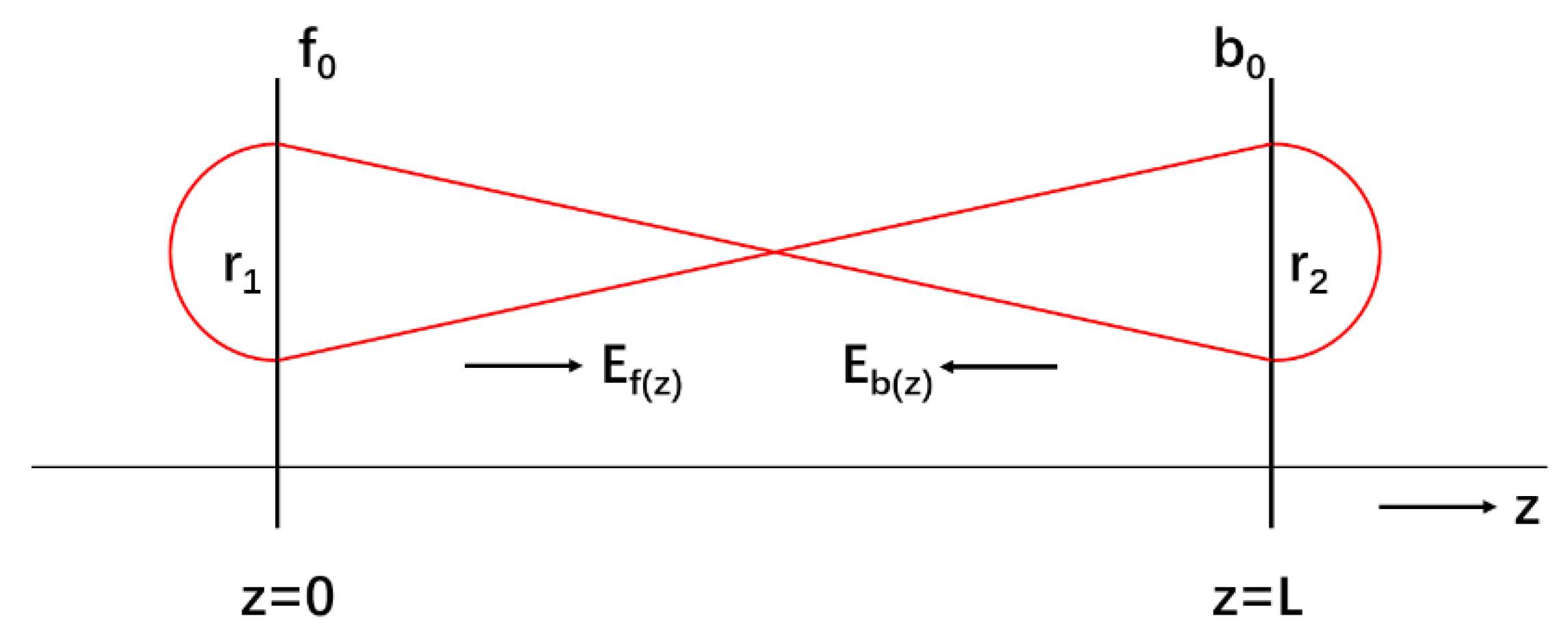
2.1. Fundamentals of Lasing Characteristics of Laser Diode (LD) with External Cavity

An example of a simplified LD structure is the Fabry–Perot-type laser, as shown in Figure 1. A stripe waveguide along the active layer is formed, and the optical wave may propagate along this waveguide until it is reflected after a length of $z=L$ at the cleaved rear endface of the laser device. Lasing characteristics may be described using the field equation approach [28]. The forward-travelling complex electrical field can be expressed as

$$E_{f\left(z\right)}=E_{f\left(0\right)}·e^{-j\frac{2\pi {\mu }_e\nu z}{c}+\frac{1}{2}\left(g-{\alpha }_s\right)z},$$

(1)

while the backward version can be expressed as

$$E_{b\left(z\right)}=E_{b\left(0\right)}·e^{-j\frac{2\pi {\mu }_e\nu \left(L-z\right)}{c}+\frac{1}{2}\left(g-{\alpha }_s\right)\left(L-z\right)},$$

(2)

with light velocity $c$ [28].

$E_{f\left(z\right)}$ and $E_{b\left(z\right)}$ are related to one another by the reflection coefficients $r_1$, $r_2$ of the laser facets, where ${\mu }_e$, denoting the effective refractive index of the LD, and $\nu =nc/2L{\mu }_e$, with the integer $n$, are the possible emission frequencies. The total gain coefficient is represented by $\left(g-{\alpha }_s\right)$.

According to the condition for a stationary laser oscillation, the field amplitude and phase should yield the following [28]:

$$\left\{\begin{array}{c}{r}_1{r}_2{e}^{-j\frac{2\pi {\mu }_e\nu L}{c}+\left(g-{\alpha }_s\right)L}=1\\ \frac{4\pi {\mu }_e\nu L}{c}=2\pi ·n\end{array}\right.,$$

(3)

In a similar way, a typical SMI system can be considered to be a structure represented by an LD laser with an external cavity, as shown in Figure 2. Then, the field amplitude and phase should yield

$$\left\{\begin{array}{c}{r}_1\left|\overline{r_2}\right|e^{\left(g-{\alpha }_s\right)L}=1\\ \frac{4\pi {\mu }_e\nu L}{c}+{\phi }_r=2\pi ·n\end{array}\right.,$$

(4)

where ${\phi }_r$ is the phase retardance caused by the roundtrip travelled within the external cavity. The effective field reflection coefficient $\overline{r_2}$ is expressed as

$$\overline{r_2}\left(\nu \right)=r_{2\mathrm{s}}+\left(1-{\left|r_{2\mathrm{s}}\right|}^2\right)r_{2\mathrm{ext}}{e}^{-j2\pi \nu {\tau }_{ext}},$$

(5)

where $r_{2\mathrm{s}}$ is the field reflection coefficient of the laser facet at $z=L$, $r_{2\mathrm{ext}}$ is the field reflection coefficient of the target surface, and ${\tau }_{ext}$ is the roundtrip time of the optical wave in the external cavity.

The parameter of the feedback level is defined as $C=\mathsf{{\rm X}}\sqrt{1-{\alpha }^2}$, with $\mathsf{{\rm X}}=\frac{{\tau }_{ext}}{{\tau }_L}{\kappa }_{ext}$ and ${\kappa }_{ext}=\frac{r_{2\mathrm{ext}}}{r_{2\mathrm{s}}}\left(1-{\left|r_{2\mathrm{s}}\right|}^2\right)$, where $\alpha$ is the linewidth enhancement factor of the LD, and ${\tau }_L$ is the trip time of the optical wave in the LD cavity. Yielding the condition of field amplitude and phase, the phase relationship of SMI can be described as

$$0=\phi \left(t\right)-{\phi }_0\left(t\right)+C·\sin \left(\phi \left(t\right)+{\tan }^{-1}\alpha \right),$$

(6)

where ${\phi }_0\left(t\right)$ represents the phase of the external roundtrip without optic feedback, and $\phi \left(t\right)$ is the aforementioned parameter with optic feedback [28].

$P_0$ represents the original emitting power of the LD, and $m$ is the modulation depth factor. Power with feedback $P_1\left(\mathrm{t}\right)$ can be approximately expressed as follows:

$$P_1\left(\mathrm{t}\right)=P_0\left(1+m·\cos \left(\phi \left(t\right)\right)\right),$$

(7)

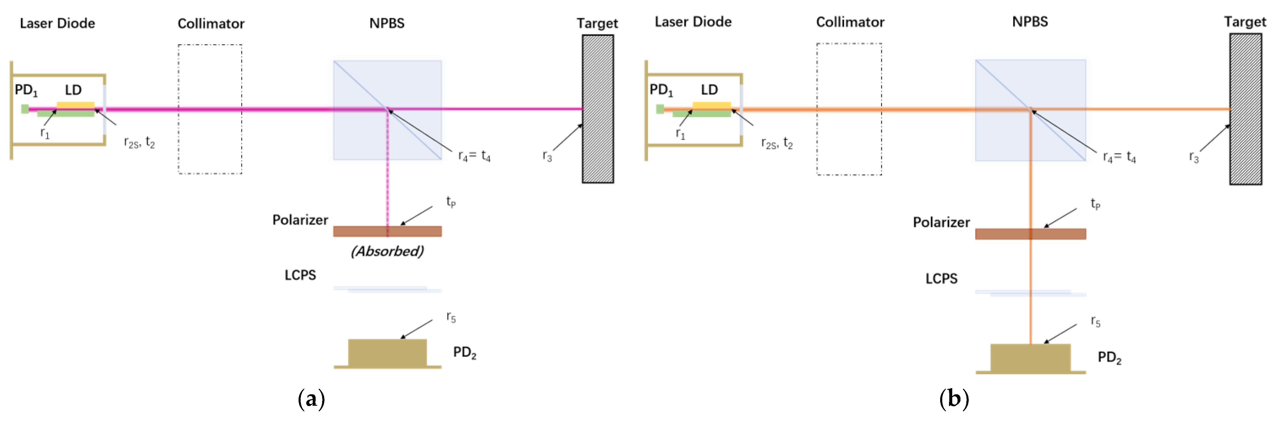
2.2. Theory of Quadrature Signal Construction in SMI Using LCPS

In order to construct quadrature signals in SMI, a $\pi /2$ phase shift should be added to the signal detected by PD2 at the front arm, while the signal detected by PD1 at the rear arm has a $\pm \pi$ phase shift [6]. In this work, we use an LCPS to shift the signal phase at the front arm by generating a certain degree of optical phase retardance. Figure 3 presents a corresponding schematic.

At the front arm, S light is absorbed by the polarizer placed between a non-polarized beam splitter (NPBS) and the LCPS. Therefore, two models are employed in this structure for S light and P light, respectively, as shown in Figure 4. For S light, the model is equivalent to a typical SMI system (Figure 4a). For P light, the model is a double external cavity SMI system (Figure 4b).

Similar to Equation (5), the effective field reflection coefficient $\overline{r_2}$ in the P light model can be written as

$$\overline{r_2}\left(\nu \right)=r_{2\mathrm{s}}+t_2{}^2{t}_4{}^2{r}_3{e}^{-j\frac{4\pi \nu L_1}{c}}+t_2{}^2{t}_4{}^2{t}_{\mathrm{p}}{}^2{r}_5{e}^{-j\frac{4\pi \nu L_2}{c}},$$

(8)

where $t_2$, $t_4$, and $t_{\mathrm{p}}$ represent the field transmittance coefficients of the LD facet, NPBS, and polarizer. The NPBS is an R:T = 50:50 type, where $r_4=t_4$. Therefore, $r_3$ is the field reflection coefficient of the target surface, while $r_5$ is that of the PD2 surface. $L_1$ is the length of the external cavity in the S light model, while $L_2=L_{21}+L_{22}$ is that of the front arm in the P light model.

For brevity, we replace $\left(g-{\alpha }_s\right)$ with $g$. PD1 receives both P light and S light, while PD2 receives S light only. The complex electrical fields $E_s$ for S light and $E_D$ for P light can be expressed as

$$E_s=s_1{E}_0·r_1{r}_{2\mathrm{s}}{e}^{-j\frac{4\pi {\mu }_e\nu L}{c}+gL}\left[1+{\kappa }_1{e}^{-j\frac{4\pi \nu L_1}{c}}\right],$$

(9)

$$E_D=s_2{E}_0·r_1{r}_{2\mathrm{s}}{e}^{-j\frac{4\pi {\mu }_e\nu L}{c}+gL}\left[1+{\kappa }_1{e}^{-j\frac{4\pi \nu L_1}{c}}+{\kappa }_2{e}^{-j\frac{4\pi \nu L_2}{c}}\right],$$

(10)

where $s_1$ and $s_2$ represent the ratio of S light to P light from the laser source, respectively. $L$ is the internal cavity length of the LD. The factors are ${\kappa }_1=t_2{}^2{t}_4{}^2{r}_3/r_{2\mathrm{s}}$, ${\kappa }_2=t_2{}^2{t}_4{}^2{t}_{\mathrm{p}}{}^2{r}_5/r_{2\mathrm{s}}$.

Then, the power received by PD1 and PD2 can be given as

$$P_1\propto {\left|\stackrel{\rightharpoonup }{E_D}+\stackrel{\rightharpoonup }{E_s}\right|}^2\approx m_1\left[1+{\kappa }_1{e}^{-j\frac{4\pi \nu L_1}{c}}\right],$$

(11)

$$P_2\propto E_D{}^2\approx m_2\left[1+{\kappa }_1{e}^{-j\frac{4\pi \nu L_1}{c}}+{\kappa }_2{e}^{-j\frac{4\pi \nu L_2}{c}}\right],$$

(12)

in which the scaling factors are

$$m_1=\frac{\sqrt{2}}{2}\left(s_1+s_2\right)E_0·r_1{r}_{2\mathrm{s}}{e}^{-j\frac{4\pi {\mu }_e\nu L}{c}+gL},$$

(13)

$$m_2=s_2{E}_0·r_1{r}_{2\mathrm{s}}{e}^{-j\frac{4\pi {\mu }_e\nu L}{c}+gL},$$

(14)

The phase relationships of quadrature SMI can be described as

$$0={\phi }_{PD1}\left(t\right)-{\phi }_0\left(t\right)+C·\sin \left({\phi }_{PD1}\left(t\right)+{\tan }^{-1}\alpha \right),$$

(15)

$$0={\phi }_{PD2}\left(t\right)-{\phi }_0\left(t\right)+C·\sin \left({\phi }_{PD2}\left(t\right)+{\tan }^{-1}\alpha \right)+\frac{{\kappa }_2}{{\kappa }_1}C·\sin \left({\phi }_2+{\tan }^{-1}\alpha \right),$$

(16)

where ${\phi }_{PD1}\left(t\right)$ and ${\phi }_{PD2}\left(t\right)$ represent the phase of the photocurrent from PD1 and PD2, respectively. ${\phi }_2$ is the phase retardance brought about by the front arm, which is controlled by the LCPS. Assuming that $\alpha =3.1$ and $C=0.8$, when ${\phi }_2=\left(-0.6151+2n\right)\pi$ (according to our calculations), a pair of quadrature signals can be obtained.

$G$ is a constant coefficient representing the power scale of the two PDs. $P_0$ is the original emitting power of the LD, and $m$ is a constant modulation depth factor. The pair of quadrature signals $I_1\left(t\right)$ and $I_2\left(t\right)$ can be obtained by cancelling the DC components of the signal as follows:

$$I_1\left(t\right)=-G{P}_{0}m\cos \left({\phi }_{PD1}\left(t\right)\right),$$

(17)

$$I_2\left(t\right)=G{P}_{0}m\cos \left({\phi }_{PD2}\left(t\right)\right)=-G{P}_{0}m\sin \left({\phi }_{PD1}\left(t\right)\right),$$

(18)

Using arctangent and unwrapping demodulation, $\mathsf{\Delta }\phi \left(t\right)$ can be calculated from $I_1$ and $I_2$. $\lambda$ is the center wavelength of the LD. As the half wavelength corresponds to the $2\pi$ phase variation, the displacement of a vibrating object can be rewritten as follows:

$$Displacement=\frac{\mathsf{\Delta }\phi \left(t\right)\lambda }{2·2\pi }=unwrap\left({\tan }^{-1}\frac{I_1\left(t\right)}{I_2\left(t\right)}\right)·\frac{\lambda }{2·2\pi }.$$

(19)

3. Simulations and Experiments

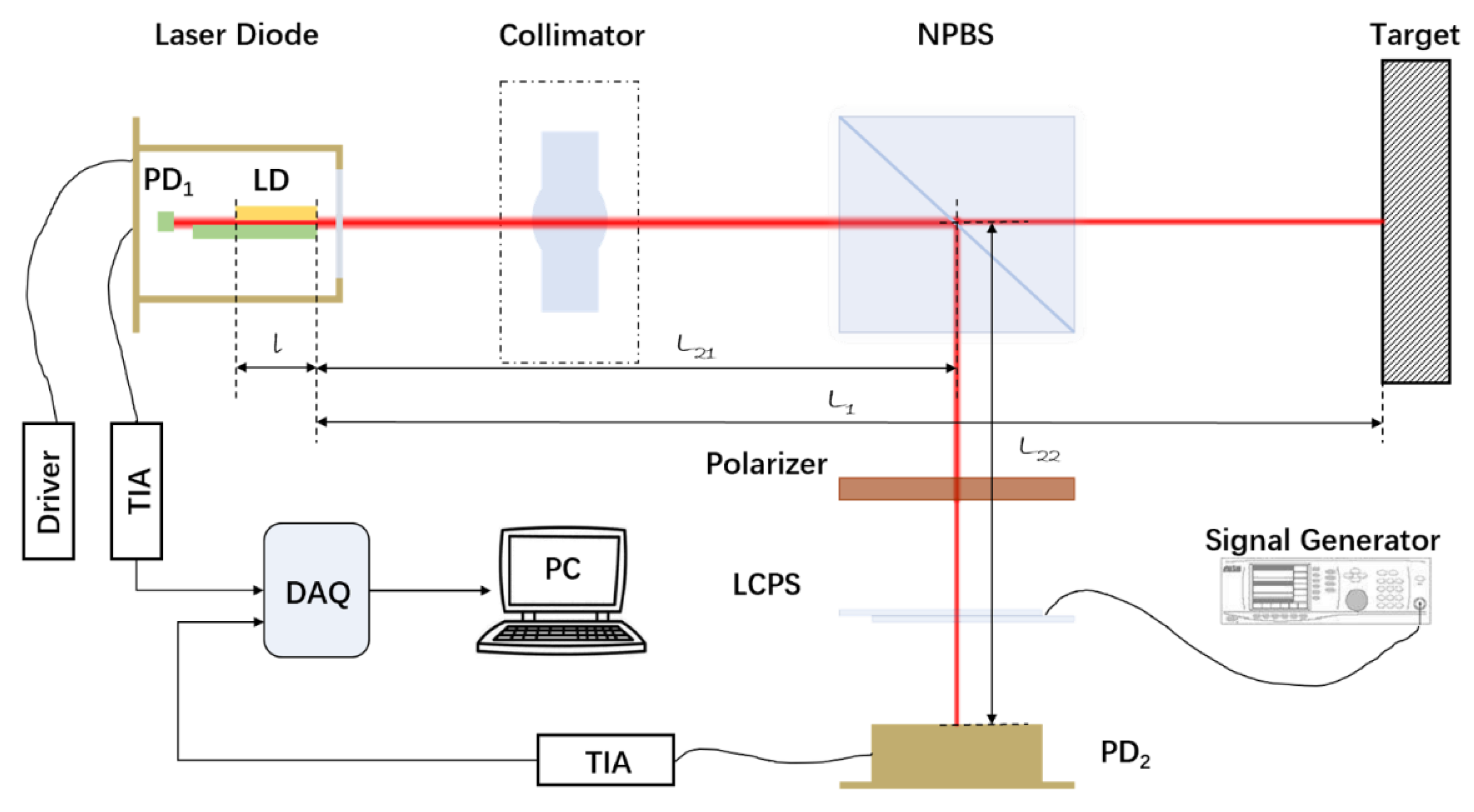
3.1. Experimental Setup

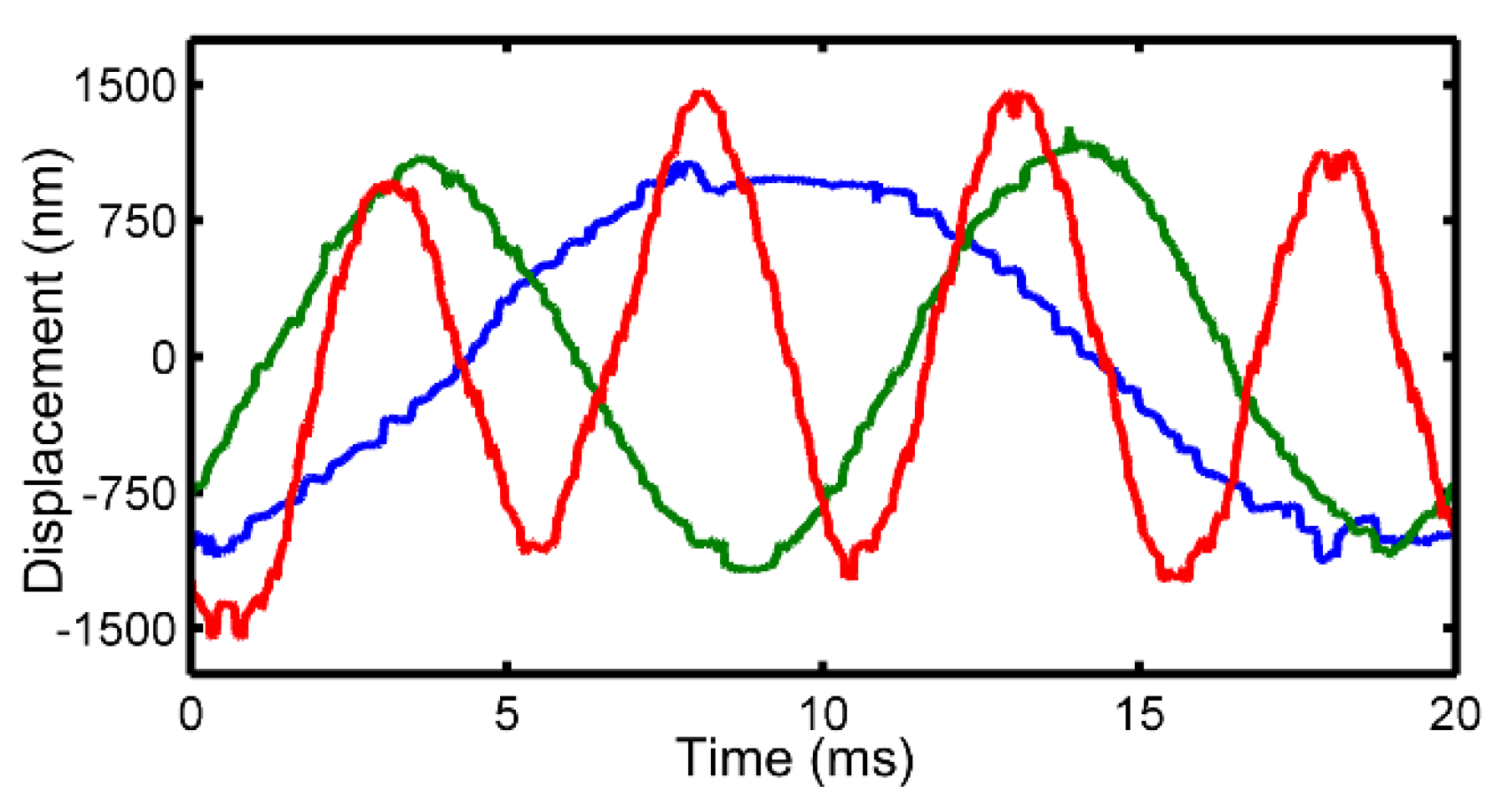
The experimental setup is shown in Figure 5. To partly avoid the unexpected emission wavelength drift caused by changes in the LD’s driving current, a single longitudinal mode laser diode (namely, RLD65NZX2 produced by ROHM, with maximum power p = 7 mW, visible wavelength λ = 650 nm, and a driven current of 39 mA) is used as the laser source. An adjustable LD collimation tube (LTN330-B by Thorlabs China, Shanghai) with an aspheric lens is placed in front of the LD to adjust the focal length. The front PD (PD2 in Figure 5) is a Si photodiode with a spectral response range of 190–1000 nm and a peak response of 0.36 A/W at 720 nm (S1226-8BQ by HAMAMATSU), while the rear PD (PD1 in Figure 5) is the LD’s built-in monitor PD. A non-polarized beam splitter with R:T = 50:50 (BS016 by Thorlabs) is positioned, and an LCPS with a gap of 5.1 μm filled with liquid crystal materials—with the ability to add phase retardance to the front-arm beam from 0 to 1.57π, for which there is an alternating drive peak–peak voltage between −5 V and 5 V of the square wave at 1 kHz—is used to construct the quadrature signals and fix the phase retardance caused by the beam splitter. A polarizer with an extinction ratio of 500:1 is placed between the beam splitter and the LCPS to attenuate the energy of the light components that are not parallel with the principal axis of the LCPS. This minimizes the amplitude modulation.

In the optical part, the emission beam including both P light and S light from the LD passes through the collimation tube and reaches the NPBS. The NPBS splits the beam into two beams, and each beam contains both P light and S light. One beam passes through the NPBS to the surface of the target, and it is reflected back to the LD through the same path from which it came, forming a typical SMI external cavity. The other beam split by the NPBS is transmitted to the front arm, and S light is attenuated by the polarizer. P light passes through the polarizer and LCPS to reach PD2, forming an external cavity in the front arm. At the front arm, a controllable degree of optical phase retardance is generated by the LCPS.

The benefit of using this scheme is that the phase difference drift caused by the alteration of the LD’s wavelength and environmental disturbance can be partly fixed, while a pair of quadrature signals can easily be acquired.

In the setup of the electrical part, a low-noise (6 nV/√Hz, 1 fA/√Hz) JFET amplifier (LT1169) is used to transfer the photocurrents from PD1 and PD2 to voltage signals. Two sets of trans-impedance amplifiers (TIAs) composed of operational amplifiers (LT1122) provide the DC bias and gain adjustment. When measuring the vibration of the loudspeaker, the LCPS is driven by a 2.51 Vpp alternative square wave with a 1 kHz frequency in order to obtain the quadrature signals.

Subsequently, the voltage signals are obtained using a synchronized data acquisition card (USB-6356 by NI) and processed on a PC. It is a quick and easy task to acquire and demodulate the signals. Therefore, measurement using this method is performed online and in real time.

3.2. Results

A small loudspeaker driven by a sinusoidal wave was used as the target. Only normalization was carried out in the preprocessing of SMI signals, as shown in Figure 6 (denoted by blue and green traces). Then, an arctangent demodulation algorithm was used to reconstruct the vibration information.

An experimental result, namely a 200 Hz vibration measurement, is shown in Figure 6. The blue and green traces show the pair of quadrature SMI signals after normalization, while the red trace shows the result of the reconstruction of the vibration information. The peak–peak values of displacement reconstructed using the proposed method and estimated using the fringe-counting method are 2288 nm and 2275 nm, respectively. The accuracy of the displacement reconstructed using the proposed method is acceptable, despite the degradation of SMI signals.

Figure 7 and Figure 8 show the results of the reconstructed displacement, in which a set of vibrations with different frequencies were detected. Low-frequency vibrations of 50 Hz, 100 Hz, and 200 Hz were detected, and the results are shown in Figure 7. The blue trace represents the reconstructed vibration information for 50 Hz, while the green and red traces represent the 100 Hz and 200 Hz vibration information, respectively. Additionally, Figure 8 shows the results for vibrations with slightly higher frequencies, i.e., 800 Hz and 1000 Hz. The blue trace represents the reconstructed vibration information of 800 Hz, and the green trace represents information for 1000 Hz. To distinguish between the two traces, we shifted the green trace negatively by 1000 nm on the vertical axis. Obviously, a resolution much better than the half wavelength of the LD was attained.

Therefore, we have verified that the proposed method can construct quadrature SMI signals using a liquid crystal phase shifter. Additionally, vibration information can be extracted from the quadrature self-mixing signals using the typical arctangent demodulation algorithm, in which quadrature signals are obtained by driving the liquid crystal phase shifter at a certain peak–peak voltage.

3.3. Simulations and Experiments under the Condition of Vibration Amplitudes near λ/4

When the amplitude of the vibration is smaller than the half wavelength of the LD, fringes will no longer be visible in SMI signals. This will nullify the effect of the methods based on fringe processing. Using the proposed method, vibrations with amplitudes far smaller than $\lambda /2$ can be measured when phase retardance is correctly provided.

However, we found a weakness in this method: when the vibration amplitude is near $\lambda /4$, a distortion in the results will occur. To determine the source of the problem, we ran a series of simulations. One of the SMI signals (Sig1) (denoted by the blue traces in Figure 9a,c) was simulated based on the numerical solution of the transcendental equation of the SMI signal phase and the target vibration phase (Equation (15)). The other SMI signal (Sig2) (denoted by the red traces in Figure 9a,c) was obtained by adding a $\pi /2$ phase shift to Sig1 to ensure that Sig1 and Sig2 corresponded to a quadrature. The feedback level was set to $C=0.8$, and the linewidth enhancement factor was set to $\alpha =3.1$. Then, we ran the arctangent demodulation algorithm to rebuild the vibration information from Sig1 and Sig2.

The simulation results presented in Figure 9b (red trace) reveal that a reconstructed displacement with a correctable amplitude attenuation has been obtained, in which the amplitude of target vibration has been set to 40 nm away from $\lambda /4$. Figure 9a presents the simulation of SMI signals.

Under the condition where the vibration amplitude was set near to $\lambda /4$, Figure 9c shows the simulated SMI signals, and Figure 9d shows the distortion mentioned above. In Figure 9b,d, the blue traces show the defined target vibration, while red traces are the simulation results of the reconstructed displacement based on simulated SMI signals.

SMI signals generated by the simulations are strictly quadrature, hence proving that the distortion was introduced by the arctangent demodulation algorithm. In Equation (6), we can notice that the jump points of phase φ(t) are in different positions when the target moves forward and backward. This behavior causes the aforementioned phenomenon.

Figure 10 shows a partial reconstruction result of a 1000 Hz vibration measurement. The vibration amplitude of the target is near λ/4, and the entire sampling time is 10 s. A 1000 Hz sinusoidal-like wave can be seen in the zoomed-in map in the upper right-hand corner of the figure. A sinusoidal vibration with an amplitude close to 1/4 of the wavelength of the LD produced a certain distortion, which is consistent with the simulation results. The FFT analysis result is shown in Figure 11, in which a component of a 1000 Hz vibration is clearly depicted.

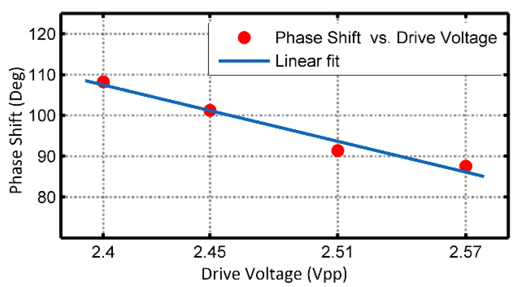
3.4. Relationship between SMI Signal Phase Difference and LCPS Drive Voltage

To confirm that the generation of the pair of final quadrature SMI signals is introduced and constrained by the total optical phase retardance at the front arm, which is controlled by the LCPS, a series of experiments and analyses were conducted.

In contrast to Equation (15), which has a typical form for SMI, Equation (16) contains an additional constant term, namely $\frac{{\kappa }_2}{{\kappa }_1}C·\sin \left({\phi }_2+{\tan }^{-1}\alpha \right).$ We defined $\mathsf{\Delta }\phi ={\phi }_{PD1}\left(t\right)-{\phi }_{PD2}\left(t\right)$ as the phase shift between the pair of SMI signals. It is obvious that $\mathsf{\Delta }\phi$ is triggered by the additional term. In the additional term, as mentioned in Section 2.2, ${\kappa }_1$ and ${\kappa }_2$ are constant coefficients that only depend on the effective field reflection coefficients and effective field transmittance coefficients of the surfaces of the LD, the NPBS, the polarizer, the LCPS, and the target. Similarly, constant coefficient $C$ represents the feedback level, and $\alpha$ represents the linewidth enhancement factor of the LD; they will become constant once the system and drive are pre-fixed. Significantly, ${\phi }_2=2\pi \upsilon {\tau }_{ext2}$ is the only tunable variable, which describes the optical phase retardance caused by the roundtrip journey of the optical wave at the front arm. ${\tau }_{ext2}=2OPL/c$ is the roundtrip transit time, where c denotes light velocity. As the other optical devices are untunable and pre-fixed, the optical path length (OPL) at the front arm is only controlled by the LCPS.

In order to determine the relationship between the phase shift $\mathsf{\Delta }\phi$ and the additional term, a numerical simulation was introduced, in which we simulated how $\mathsf{\Delta }\phi$ changes with the additional term. The simulated phase ${\phi }_{PD1}\left(t\right)$ of the signal from PD1 was obtained by calculating Equation (15) with any given target vibration, while ${\phi }_{PD2}\left(t\right)$ is the numerical solution of Equation (16) in the domain [−2, 2] (radian) of the additional term. Then, $\mathsf{\Delta }\phi$ can be calculated. The simulation result is shown in Figure 12, where the horizontal axis represents the variation of the additional term, and the longitudinal axis represents the variation in the dependent variable $\mathsf{\Delta }\phi$. Obviously, there is a strict positive correlation between $\mathsf{\Delta }\phi$ and the additional term. It is easy to determine that $\mathsf{\Delta }\phi =\pi /2$ (90°) when the value of the additional term is 1.471 rad, and it becomes $\mathsf{\Delta }\phi =-\pi /2$ (−90°) when the value of the additional term becomes −1.497 rad.

According to the simulation above, the optical path length (OPL) at the front arm is only controlled by the LCPS.

At this stage, experiments with other identical conditions were introduced. We tuned the amplitude of the LCPS drive voltage to verify that the LCPS in this system leads to a controllable SMI signal phase modulation. The different drive voltages tune the phase retardance between the two SMI signals from PD1 and PD2. The two SMI signals were preprocessed using a normalization algorithm, and they have the same frequency. Hence, the phase shift $\mathsf{\Delta }\phi$ was calculated from the ellipticity of the Lissajous figures formed by the two normalized SMI signals from PD1 and PD2 in each period.

As shown in Figure 13, 1200 sets of data were acquired for each drive voltage of the LCPS. The bottom and top edges of the box indicate the 25th and 75th percentiles, and the red line is the median position. Except for some abnormal points, most of the phase retardance is concentrated within ±5° of the median. The phase shift has a linear relationship with the drive voltage of the LCPS, as shown in Figure 14, and there is an approximately linear range with an R-square of 0.9707 and an RMSE of 1.9677. For other vibration measurements in this work, we set the LCPS drive voltage to 2.51 Vpp to obtain two sets of photocurrent signals with approximate phase quadrature.

4. Discussion

The feasibility of our proposed method was verified by the simulation and experimental results. The proposed method allows one to construct quadrature SMI signals based on the principle of the superposition of the crossed optical field occurring at the LD’s built-in monitor PD1. In contrast to the methods outlined by the authors of [13,21], who constructed quadrature SMI signals or a multidimensional displacement measurement system using polarization multiplexing (PM) or wavelength division multiplexing (WDM) techniques, in this method, SMI signals with a desired phase shift are obtained by modulating the total light intensity, including both P light and S light, received by PD1 using an LCPS in the front arm. Inspired by the work on quadrature detection for self-mixing interferometry [27], we have explained and demonstrated a method for constructing quadrature SMI signals without using PM or WDM techniques. Therefore, it has a more concise structure and a lower cost. It is worth noting that phase retardance between the two ‘quadrature’ SMI signals is disturbed by environmental disturbance such as variations in temperature and local vibrations. The influence of environmental disturbance will be investigated in future works.

5. Conclusions

In conclusion, we have proposed a novel method for quadrature signal construction in SMI. Theoretical explanations were provided. Furthermore, simulations and experiments were carried out to verify the feasibility of the proposed method. Using this method, it is possible to reconstruct the displacement of vibrating objects using a quadrature detection technique. In this work, quadrature detection also cancels any reference signals such as normal IQ demodulation. It simplifies the calculation process of SMI signal demodulation. This technique can be applied to several SMI measurements for online and real-time micro vibration monitoring such as surface deviation measurements and residual vibration measurements.

References

1. Contreras, V.; Toivonen, J.; Martinez, H. Enhanced self-mixing interferometry based on volume Bragg gratings and laser diodes emitting at 405-nm wavelengths. Opt. Lett. 2017, 42, 2221. [Google Scholar] [CrossRef]
2. Giuliani, G.; Norgia, M.; Donati, S.; Bosch, T.J. Laser diode self-mixing technique for sensing applications. Opt. A 2002, 4, S283. [Google Scholar] [CrossRef]
3. Donati, S. Developing self-mixing interferometry for instrumentation and measurements. Laser Photon. Rev. 2012, 6, 393. [Google Scholar] [CrossRef]
4. Guo, D.; Shi, L.; Yu, Y.; Xia, W.; Wang, M. Micro-displacement reconstruction using a laser self-mixing grating interferometer with multiple-diffraction. Opt. Express 2017, 25, 31394. [Google Scholar] [CrossRef] [PubMed]
5. Shi, L.; Guo, D.; Cui, Y.; Hao, H.; Xia, W.; Wang, Y.; Ni, X.; Wang, M. Design of a multiple self-mixing interferometer for a fiber ring laser. Opt. Lett. 2018, 43, 4124. [Google Scholar] [CrossRef] [PubMed]
6. Li, K.; Cavedo, F.; Pesatori, A.; Zhao, C.; Norgia, M. Balanced detection for self-mixing interferometry. Opt. Lett. 2017, 42, 283. [Google Scholar] [CrossRef]
7. Magnani, A.; Pesatori, A.; Norgia, M. Real-time Self-mixing interferometer for long distances. IEEE Trans. Instrum. Meas. 2014, 63, 1804. [Google Scholar] [CrossRef]
8. Jiang, C.; Geng, Y.; Liu, Y.; Liu, Y.; Chen, P.; Yin, S. Rotation velocity measurement based on self-mixing interference with a dual-external-cavity single-laser diode. Appl. Opt. 2019, 58, 604. [Google Scholar] [CrossRef]
9. Yáñez, C.; Azcona, F.; Royo, S. Confocal flowmeter based on self-mixing interferometry for real-time velocity profiling of turbid liquids flowing in microcapillaries. Opt. Express 2019, 27, 24340. [Google Scholar] [CrossRef]
10. Gao, B.; Qing, C.; Yin, S.; Peng, C.; Jiang, C. Measurement of rotation speed based on double-beam self-mixing speckle interference. Opt. Lett. 2018, 43, 1531. [Google Scholar] [CrossRef]
11. Qi, P.; Zhou, B.; Zhang, Z.; Li, S.; Li, Y.; Zhong, J. Phase-sensitivity-doubled surface plasmon resonance sensing via self-mixing interference. Opt. Lett. 2018, 43, 4001. [Google Scholar] [CrossRef] [PubMed]
12. Norgia, M.; Pesatori, A.; Donati, S. Compact laser-diode instrument for flow-measurement. IEEE Trans. Instrum. Meas. 2016, 65, 1478. [Google Scholar] [CrossRef]
13. Li, J.; Tan, Y.; Zhang, S. Generation of phase difference between self-mixing signals in a-cut Nd:YVO4 laser with a waveplate in the external cavity. Opt. Lett. 2015, 40, 3615–3618. [Google Scholar] [CrossRef] [PubMed]
14. Xu, Z.; Li, J.; Zhang, S.; Tan, Y.; Zhang, X.; Lin, X.; Wan, X.; Zhuang, S. Remote eavesdropping at 200 meters distance based on laser feedback interferometry with single-photon sensitivity. Opt. Lasers Eng. 2021, 141, 106562. [Google Scholar] [CrossRef]
15. Zhao, Y.; Zhou, J.; Wang, C.; Xiang, R.; Bi, T.; Lu, L. Design and application research of the multi-longitudinal mode laser self-mixing vibration measurement system. Measurement 2019, 114, 381. [Google Scholar] [CrossRef]
16. Wang, C.; Fan, X.; Guo, Y.; Gui, H.; Wang, H.; Liu, J.; Yu, B.; Lu, L. Full-circle range and microradian resolution angle measurement using the orthogonal mirror self-mixing interferometry. Opt. Express 2018, 26, 10371. [Google Scholar] [CrossRef]
17. Xiang, R.; Yu, B.; Lu, L. Real-time vibration monitoring system of thin-walled structures’ health status based on the self-mixing effect. In Proceedings of the International Conference on Optical Instruments and Technology 2017: Advanced Optical Sensor and Applications, Beijing, China, 2018; Volume 10618. [Google Scholar]
18. Wang, B.; Liu, B.; An, L.; Tang, P.; Ji, H.; Mao, Y. Laser Self-Mixing Sensor for Simultaneous Measurement of Young’s Modulus and Internal Friction. Photonics 2021, 8, 550. [Google Scholar] [CrossRef]
19. Guo, D.; Xie, Z.; Yang, Q.; Xia, W.; Yu, Y.; Wang, M. Self-Mixing Interferometry Cooperating with Frequency Division Multiplexing for Multiple-Dimensional Displacement Measurement. Photonics 2023, 10, 839. [Google Scholar] [CrossRef]
20. Liu, B.; Ruan, Y.; Yu, Y. Determining System Parameters and Target Movement Directions in a Laser Self-Mixing Interferometry Sensor. Photonics 2022, 9, 612. [Google Scholar] [CrossRef]
21. Wang, X.; Zhong, Z.; Chen, H.; Zhu, D.; Zheng, T.; Huang, W. High-Precision Laser Self-Mixing Displacement Sensor Based on Orthogonal Signal Phase Multiplication Technique. Photonics 2023, 10, 575. [Google Scholar] [CrossRef]
22. Tao, Y.; Xia, W.; Wang, M.; Guo, D.; Hao, H. Integration of polarization-multiplexing and phase-shifting in nanometric two dimensional self-mixing measurement. Opt. Express 2017, 25, 2285. [Google Scholar] [CrossRef] [PubMed]
23. Zhang, Z.; Li, C.; Huang, Z. Quadrature demodulation based on lock-in amplifier technique for self-mixing interferometry displacement sensor. Appl. Opt. 2019, 58, 6098. [Google Scholar] [CrossRef] [PubMed]
24. Zhang, Z.; Li, C.; Huang, Z. Vibration measurement based on multiple Hilbert transform for self-mixing interferometry. Opt. Commun. 2019, 436, 192. [Google Scholar] [CrossRef]
25. Fan, Y.; Yu, Y.; Xi, J.; Chicharo, J. Improving the measurement performance for a self-mixing interferometry-based displacement sensing system. Appl. Opt. 2011, 50, 5064. [Google Scholar] [CrossRef]
26. Wang, X.; Yuan, Y.; Sun, L.; Gao, B.; Chen, P. Self-mixing interference displacement measurement under very weak feedback regime based on integral reconstruction method. Opt. Commun. 2019, 445, 236. [Google Scholar] [CrossRef]
27. Wu, J.; Shu, F. Quadrature detection for self-mixing interferometry. Opt. Lett. 2018, 43, 2154. [Google Scholar] [CrossRef]
28. Petermann, K. Basic Laser Characteristics. In Laser Diode Modulation and Noise; Kluwer: Dordrecht, The Netherlands, 1988; Volume 3, pp. 25–26. [Google Scholar]
Figure 1. Electrical field flow in forward and backward directions in a semiconductor laser with facet field reflectivity coefficients r1,r2.
Photonics 10 01121 g001
Figure 2. Schematic of the simplified SMI system.
Photonics 10 01121 g002
Figure 3. Schematic of the quadrature SMI system using LCPS. The red line represents laser beam.
Photonics 10 01121 g003
Figure 4. Models for S light and P light in quadrature SMI system: (a) for S light; (b) for P light. The purple line represents S light, and orange one represents P light.
Photonics 10 01121 g004
Figure 5. Schematic of the experimental setup.
Photonics 10 01121 g005
Figure 6. Acquired SMI signals and the reconstructed displacement. The sinusoidal-like trace is the calculated displacement, while the other two traces are normalized SMI signals obtained from processing the monitored PD (PD1) output and front PD (PD2) output.
Photonics 10 01121 g006
Figure 7. The rebuilt micro-displacements of low-frequency vibrations. The three traces are measurement results of vibrations with frequencies of 50 Hz, 100 Hz, and 200 Hz, respectively.
Photonics 10 01121 g007
Figure 8. The rebuilt micro-displacements of slightly higher-frequency vibrations. The two traces are measurement results of vibrations with frequencies of 800 Hz and 1000 Hz, respectively.
Photonics 10 01121 g008
Figure 9. The simulation results of small amplitude vibrations. (a) The pair of simulated quadrature SMI signals with a 40 nm vibration; (b) the given target vibration and the rebuilt displacement based on SMI signals in (a); (c) the pair of simulated quadrature SMI signals of vibration with an amplitude near λ/4 (160 nm); (d) the given target vibration and the rebuilt displacement based on SMI signals in (c).
Photonics 10 01121 g009
Figure 10. Partial reconstruction result of a 1000 Hz vibration measurement. The box in the upper right corner of the square is a zoomed-in map of the micro-displacement.
Photonics 10 01121 g010
Figure 11. The FFT analysis result of micro-displacement with a frequency of 1000 Hz.
Photonics 10 01121 g011
Figure 12. The simulation results of the relationship between the phase shift Δ φ and the additional term.
Photonics 10 01121 g012
Figure 13. The difference in the SMI signal phase shift between monitor PD (PD1) output and front PD (PD2) output obtained with different liquid crystal drive voltages.
Photonics 10 01121 g013
Figure 14. The linear fitting results regarding phase shift vs. drive voltage.
Photonics 10 01121 g014
Disclaimer/Publisher’s Note: The statements, opinions and data contained in all publications are solely those of the individual author(s) and contributor(s) and not of MDPI and/or the editor(s). MDPI and/or the editor(s) disclaim responsibility for any injury to people or property resulting from any ideas, methods, instructions or products referred to in the content.